Article

Possible Scenarios of Winter Wheat Yield Reduction of Dryland Qazvin Province, Iran, Based on Prediction of Temperature and Precipitation Till the End of the Century

1
Department of Water Engineering, Faculty of Engineering and Technology, Imam Khomeini International University, 3414896818 Qazvin, Iran
2
Department of Crop Sciences, Faculty of Agricultural Sciences, Georg-August University of Göttingen, Büsgenweg 5, 37077 Göttingen, Germany
3
Department of Soil Science, University of Kassel, Nordbahnhofstr. 1a, 37213 Witzenhausen, Germany
*
Author to whom correspondence should be addressed.
Climate 2018, 6(4), 78; https://doi.org/10.3390/cli6040078
Submission received: 31 August 2018 / Revised: 19 September 2018 / Accepted: 21 September 2018 / Published: 23 September 2018
(This article belongs to the Special Issue Sustainable Agriculture for Climate Change Adaptation)

Abstract

:
The climate of the Earth is changing. The Earth’s temperature is projected to maintain its upward trend in the next few decades. Temperature and precipitation are two very important factors affecting crop yields, especially in arid and semi-arid regions. There is a need for future climate predictions to protect vulnerable sectors like agriculture in drylands. In this study, the downscaling of two important climatic variables—temperature and precipitation—was done by the CanESM2 and HadCM3 models under five different scenarios for the semi-arid province of Qazvin, located in Iran. The most efficient scenario was selected to predict the dryland winter wheat yield of the province for the three periods: 2010–2039, 2040–2069, and 2070–2099. The results showed that the models are able to satisfactorily predict the daily mean temperature and annual precipitation for the three mentioned periods. Generally, the daily mean temperature and annual precipitation tended to decrease in these periods when compared to the current reference values. However, the scenarios rcp2.6 and B2, respectively, predicted that the precipitation will fall less or even increase in the period 2070–2099. The scenario rcp2.6 seemed to be the most efficient to predict the dryland winter wheat yield of the province for the next few decades. The grain yield is projected to drop considerably over the three periods, especially in the last period, mainly due to the reduction in precipitation in March. This leads us to devise some adaptive strategies to prevent the detrimental impacts of climate change on the dryland winter wheat yield of the province.

1. Introduction

The temperature of the Earth is increasing more rapidly than during the previous decades, leading to extensive climate change [1]. The Earth’s temperature is projected to maintain its upward trend slightly in the next few decades [1]. A significant rise in the concentration of greenhouse gases such as CO2, CH4, N2O, and water vapor, mainly caused by human activities, has intensified this trend [2]. The concentration of greenhouse gases, volume of ozone, aerosols, and sunspots seem to be the most noticeable reason for temperature variations and climate change in the recent century [3].
More than two billion people live in drylands, constituting nearly 40% of the world’s population [4]. Cereals are the major crops cultivated in drylands [5]. Crop production in drylands mainly depends on precipitation during the growing season [6]. Moreover, the rise in temperature has led to exacerbating droughts and a considerable loss in crop yields in arid and semi-arid regions [7]. It is necessary to manage drylands in a sustainable way, by which food security is achieved [8]. To do so, there must be some possible measurements and predictions to protect vulnerable sectors such as agriculture and water resources in drylands [9].
General Circulation Models (GCMs) are the most developed tools for the simulation of general responses to the accumulation of greenhouse gases [10]. Studies have shown that the results of GCMs cannot be exploited directly because they are not accurate enough in describing sub-grid data [10]. Therefore, Statistical Downscaling Models (SDSMs) are one of the tools that have been developed to deal with this problem [11]. SDSMs are the most frequently used models in agricultural research, where some independent variables are measured and collected to predict dependent variables [12]. Tatsumi et al. [13] applied the Hadley Centre Coupled Model (version 3; HadCM3) and Coupled Global Climate Model 3 (CGCM3) to forecast the daily minimum, maximum, and average temperature of Shikoku city in Japan, using downscaling techniques. Their results indicated that the temperature is likely to increase in the Shikoku region, Japan, within the period 2071–2099. In a similar study, Ribalaygua et al. [14] used downscaling techniques to simulate the daily minimum and maximum temperature and daily precipitation in a region located in Spain. Their results showed that maximum and minimum temperatures will rise, while precipitation will decrease in the 21st century. Johns et al. [15], by applying the HadCM3 model, predicted that some regions of Central America and Southern Europe might be moister in the future, whereas Australia may experience a type of drier climate.
In recent years, researchers have studied the potential impacts of climate change on plant growth by using different types of simulation models [16,17]. Russell et al. [18] reported that most of the alterations in wheat yield in the United States are related to climate change. Temperature and precipitation, as two important climatic variables for the evaluation of future grain yield, have been investigated by many researchers. For instance, [16] indicated that the changes in temperature and precipitation within the last 30 years in Mexico had positively impacted on the winter wheat yield. In another study, Landau et al. [19], by applying a multiple-regression model, indicated that the temperature increase led to an improvement in the winter wheat crop characteristics, while the precipitation increase could have negative impacts.
The downscaling of GCMs parameters and studying the possible changes in wheat yield due to climatic effects have been distinctly investigated [14,20]. Lhomme et al. [21], for example, studied the potential effect of climate change on durum wheat yield in Tunisia using the downscaled values of some scenarios. Moreover, the efficiency of the IPCC scenarios has rarely been evaluated and compared [22]. In the present study, the downscaling of two important climatic parameters—temperature and precipitation—was done by the Canadian Earth System Model (CanESM2) and HadCM3 models for the province of Qazvin, located in Iran, where the climate is semi-arid and the dryland farming of winter wheat dominates. Then, the most efficient scenario was chosen to predict the dryland winter wheat yield of the province for the next few decades through a multiple-regression model. The efficiency of the fourth and fifth IPCC scenarios in predicting the temperature and precipitation of the region was also compared.

2. Materials and Methods

2.1. Geography, Climate, and Dryland Farming of the Province

The province of Qazvin has an area of 15,821 km², located between 48–45 to 50–50 East of the Greenwich Meridian of longitude and 35–37 to 36–45 North latitude of the Equator. Its average altitude is 1278 m above sea level. It has a semi-arid climate with the annual mean precipitation, daily mean temperature, and relative humidity of 301 mm, 14.2 °C, and 51%, respectively. The province is affected by Siberian and Mediterranean winds, which are considerably important factors in controlling the climate of the province. The geographical situation of the studied area is shown in Figure 1.
The total winter wheat yield of the province is 445 million kg, 364 million kg (82%) of which belongs to irrigated farming and 80.7 million kg (18%) to dryland farming. The total cultivated area for winter wheat is nearly 202,497 ha, 95792 ha and 106,704 ha of which are under irrigated and dryland farming, respectively. The average dryland winter wheat yield of the province is estimated to be 1541 kg ha−1.

2.2. Methodology

The daily mean temperature and precipitation data for 32 years (1985–2017) were collected from the six meteorological stations in the province (Figure 1). Thereafter, the daily mean temperature and precipitation of all days of all years were calculated separately by the Thiessen polygons method using the software ArcGIS version 10 via Equations (1) and (2):
P a = p i A i A i
T a = t i A i A i
where P a and T a are the daily mean precipitation and temperature of the province, respectively; pi and ti are the daily mean precipitation and temperature in the station i, respectively; and Ai is the area of the province.
The HadCM3 and CanESM2 models were used to compare the scenarios. HadCM3 has a spatial resolution of 2.5° × 3.75° (latitude by longitude) and the representation produces a grid box resolution of 96 × 73 grid cells. This produces a surface spatial resolution of about 417 km × 278 km, reducing to 295 km × 278 km at 45 degrees North and South. In CanESM2, the long-term time series of standardized daily values are extracted into a one column text file per grid cell. The 128 × 64 grid cells cover global domain according to a T42 Gaussian grid. This grid is uniform along the longitude with a horizontal resolution of 2.81° and is nearly uniform along the latitude of roughly 2.81°. The calibration of the stations (points) against the grid-cells (pixels) was done by the downscaling of the SDSM linear regression model. Data from the years 2006–2015 and 2016–2017 were used for the calibration and validation of both models, respectively.
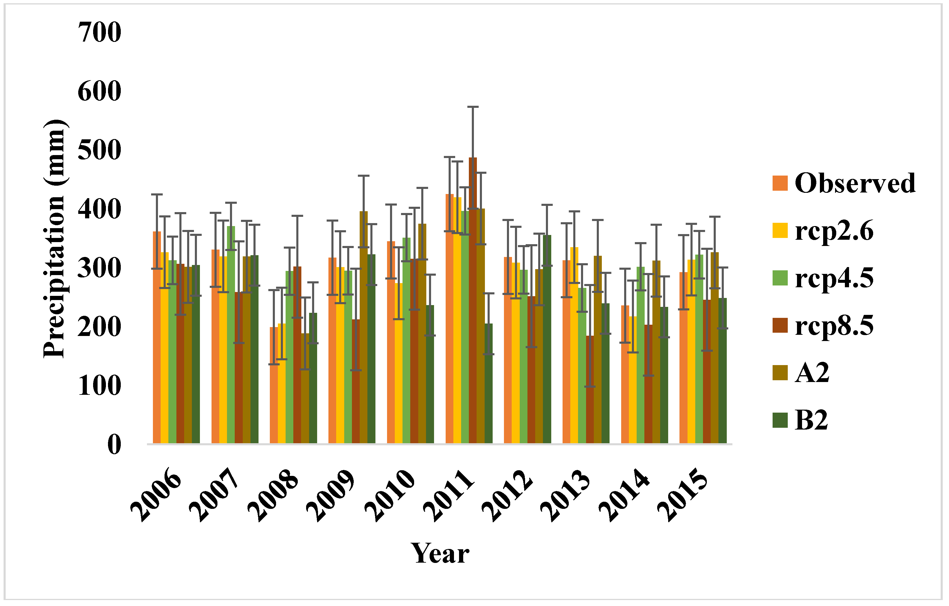
 Figure 2 and Figure 3 show the observed versus the simulated values of the temperature and precipitation for the years 2006–2015. Meanwhile, since 26 synoptic variables are considered as predictor variables in these models, having a unique equation was not logically possible because of the accumulated error. To solve this problem, only the predictor variables, being more correlative with the daily mean precipitation and temperature than others, were chosen. Then, the correlation between the variables was detected by Pearson’s correlation test (p < 0.01) and the most important variables were selected according to the statistical significance between them and the dependent variables (p < 0.01). To analyze the climatic data across the study, it was necessary to apply a Statistical Downscaling Model (SDSM). To do so, SDSM version 5.2 was used. SDSM is a decision support tool for assessing local climate change impacts using a powerful statistical downscaling technique. It has the potential to rapidly develop downscaled climatic data [11]. To make statistical connections between the predictor and predicted variables, some regression equations were acquired to predict the climatic variables for the next few periods under the impact of climate change. After acquiring the regression equations and measuring their accuracy, the scenarios were produced through both models for the periods 2010–2039, 2040–2069, and 2070–2099. The properties of these scenarios are indicated in Table 1.
The efficiency of the scenarios was compared and the most efficient scenario was recognized through the statistical indicators of Mean Absolute Error (MAE), Root Mean Square Error (RMSE), Nash-Sutcliffe coefficient (NS), Coefficient of Determination (R2), and Analysis of Variance (at p < 0.01) as follows:
Z i = P i P ¯ σ p or   Z i = O i O ¯ σ o
MAE = i = 1 n | P i O i n |
RMSE = i = 1 n ( P i O i ) 2 n
NS = 1 ( i = 1 n ( O i P i ) 2 i = 1 n ( O i O ¯ ) 2 )
R 2 = [ 1 n i = 1 n ( Pi P ¯ ) ( Oi O ¯ ) σ p × σ o ]
where Zi is the standardized daily mean precipitation or temperature values; Oi and Pi are the observed and simulated daily mean precipitation or temperature values, respectively; O ¯ is the average of the observed daily mean precipitation or temperature values; P ¯ is the average of the simulated daily mean precipitation or temperature values; σO is the variance of the observed daily mean precipitation or temperature values; σP is the variance of the simulated daily mean precipitation and temperature values; and n is the number of data.
Isaaks and Serivastava [23] suggested the MAE and RMSE as statistical indicators able to compare the accuracy of variables. Once the MAE and RMSE values are closer to zero in a scenario, the scenario would be more efficient for predicting climatic variables [24]. When they are exactly 0, it means that there is no error in the predicting task [24]. The Nash-Sutcliffe coefficient (NS) shows to what extent the regression line between the simulated data and measured data can be similar to the regression line 1:1. Its domain is from the negative infinity to 1, and NS = 1 reveals either a complete similarity or a perfect efficiency of a scenario [25]. Meanwhile, R2 gives information on the correlation between the observed and predicted data and its domain is from 0 to 1 [26]. When R2 becomes closer to 1, there will be a significant correlation between the data groups [26]. Significant differences between the observed data and values of the predictor scenarios can be distinguished by the analysis of variance [27]. Lack of any significant difference reveals a similarity between the predicted and observed data. In addition, to obtain more appropriate results for the prediction of precipitation, the occurrence of precipitation approach was used. This is a dichotomous method by which the accuracy of whether the occurrence or non-occurrence of precipitation is evaluated. If there is no occurrence of precipitation, then the answer is ‘NO’, while the answer ‘Yes’ is a sign of precipitation occurrence [28]. There are four statuses when the observed data are compared with scenario predictions, where a couple of predictions could be true and the remaining predictions could be false. The scenario with a higher percentage of true predictions was selected as the most efficient scenario for predicting the precipitation.
Finally, to predict the dryland winter wheat yield of the province for the next decades and to make a connection between the climatic and yield data for the period 2005–2014, a linear regression model was used. Furthermore, Pearson’s correlation test (at p < 0.01) between the simulated and observed data, RMSE, and R-square were used to check the regression’s validity. All statistical analyses were performed by the software SPSS version 21 (IBM Inc., Chicago, IL, USA).

3. Results

3.1. Temperature Predictions

All three CanESM2 scenarios predicted that the daily mean temperatures would generally increase in the periods 2010–2039, 2040–2069, and 2070–2099 (Table 2). However, the scale of these increases differed by the different scenarios. The scenario rcp2.6 projected that the daily mean temperature of the periods 2010–2039, 2040–2069, and 2070–2099 would be 13.6, 13.9, and 13.9 °C, respectively, which are 0.9, 1.2, and 1.1 °C higher when compared to the observed daily mean temperature. The other scenario rcp4.5 also predicted an increasing trend in the daily mean temperature in the three prospective periods and showed that the mean daily temperature would be 13.4, 14.2, and 14.4 °C in the periods 2010–2039, 2040–2069, and 2070–2099, respectively, each being 0.7, 1.4, and 1.6 °C higher when compared to the observed one. The scenario rcp8.5 predicted the highest temperature trends in comparison with the other two scenarios. It predicted that the mean daily temperature would rise by 13.8, 14.8, and 15.5 °C in the periods 2010–2039, 2040–2069, and 2070–2099, with changes of 1.0, 2.0, and 2.7 °C, respectively, in analogy with the observed value.
Both scenarios (A2 and B2) of HadCM3 generally predicted an increasing daily mean temperature trend for the three future periods in comparison with the observed one, except for scenario B2, which projected a very slightly decreasing trend only for the period 2070–2099 (Table 3). The scenario A2 forecasted that the mean daily temperature would rise to 12.7, 12.8, and 12.8 °C in the periods 2010–2039, 2040–2069, and 2070–2099, being 0.0, 0.1, and 0.2 °C higher, respectively, when compared to the value of the observed period. The mean daily temperatures were projected by the scenario B2 to increase to 12.6 and 12.7 °C in the periods 2010–2039, 2040–2069, respectively. In contrast, it predicted that the mean daily temperature would decrease to 12.6 °C in the period 2070–2099. Accordingly, the predicted temperature changes by scenario B2 are 0.02, 0.05, and −0.04 °C in the periods 2010–2039, 2040–2069, and 2070–2099, respectively, when compared to the observed period.

3.2. Precipitation Predictions

Overall, the three scenarios of CanESM2 projected a diminishing trend in the annual precipitation for the future periods 2010–2039, 2040–2069, and 2070–2099, when compared to the observed period (Table 4). However, the scenario rcp2.6 projected a less decreasing trend in the annual precipitation for the period 2070–2099. The scenario rcp2.6 predicted that the annual precipitation would drop to 287 and 277 mm in the periods 2010–2039 and 2040–2069, respectively, and decrease to 296 mm in the period 2070–2099. The projected annual precipitation by the scenario rcp4.5 would be 258, 264, and 293 mm in the periods 2010–2039, 2040–2069, and 2070–2099, respectively. The other scenario rcp8.5 forecasted that the annual precipitation would be 283, 278, and 278 mm for the periods 2010–2039, 2040–2069, and 2070–2099, respectively.
Scenario A2 of HadCM3 predicted a decreasing trend in the annual precipitation for the periods 2010–2039, 2040–2069, and 2070–2099, in analogy with the observed period (Table 5). The annual precipitation projected by scenario A2 would be 340, 292, and 276 mm for the periods 2010–2039, 2040–2069, and 2070–2099, respectively. Scenario B2 also forecasted that the annual precipitation for the periods 2010–2039 and 2040–2069 would be 310 and 321 mm, respectively, when compared to the observed period, which conveys a reducing trend. In contrast, it projected an increased annual precipitation of 875 mm for the period 2070–2099, which will be noticeably higher than the observed amount.

3.3. Comparison of the Scenarios

The variance analysis results showed a higher efficiency for the RCP scenarios than the A and B scenarios in predicting the daily mean temperature of the region (Table 6), because there was no statistically significant difference between the temperature values simulated by the RCPs and the observed values (at p < 0.01), while the temperature values simulated by A and B significantly differed from the observed ones (at p < 0.01). Among the three scenarios of the model CanESM2, rcp2.6 was selected as the most efficient scenario for predicting the daily mean temperature, as it had the highest Nash-Sutcliffe coefficient and R2 value and the lowest MAE and RMSE values when compared to scenarios rcp4.5 and rcp8.5.
The results of variance analysis indicated that all scenarios were efficient enough to predict the annual precipitation of the region (Table 7), since no statistically significant difference was found between the simulated and observed values (at p < 0.01). The scenario rcp2.6 displayed the lowest values for both MAE and RMSE. Moreover, it showed the highest Nash-Sutcliffe coefficient and R2 value. Thus, it was selected as the best scenario for predicting the annual precipitation. In addition, the scenarios of CanESM2 simulated closer annual precipitation values to the observed values than the HadCM3 scenarios (Table 8). The CanESM2 scenarios resulted in higher values of true predictions and lower values of false prediction than the scenarios of HadCM3. The indicators provided in Table 8 also, in general, confirmed the excellence of scenario rcp2.6 for predicting the annual precipitation.
Together, these indicators showed a relatively higher efficiency for the CanESM2 scenarios than the HadCM3 scenarios in predicting the daily mean temperature and annual precipitation of the region.

3.4. Yield Predictions

The results of the regression analysis and Pearson’s correlation test showed that the precipitation in March was the most effective factor for the dryland winter wheat yield of the region (Table 9). The prediction results indicated that the yield would noticeably reduce to 1176, 984, and 890 kg ha−1 in the periods 2010–2039, 2040–2069, and 2070–2099, respectively (Table 10). The reduction percentage in the above-mentioned periods is predicted to be −22, −34, and −41%, respectively. These reductions in the yield are consistent with the reductions in the mean precipitation in March during the three prospective periods (Figure 4). The reduction in the yield in the periods 2040–2069 and 2070–2099 will be more severe than that of the period 2010–2039, which is in line with a more severe reduction in the precipitation in March than in the former periods.

4. Discussion

4.1. Temperature Predictions

GCMs have widely been used for predicting future temperature trends. Van Vuuren et al. [29] showed that the mean temperature was likely to increase in the future in many parts of the world. For instance, Basheer et al. [30] claimed that the climate over the Dinder River Basin would be warmer in the upcoming decades. Majhi and Pattnayak [31] also revealed that there would be a gradual temperature increase in Nabarangpur district at the end of the 21st century. Our results also indicated that the temperature would generally increase in the three investigated periods; however, the magnitude of these increases are dependent on the scenarios applied. The CanESM2 scenarios postulated a higher variability in the predicted temperature values than the HadCM3 scenarios. In addition, the temperature changes predicted by CanESM2 were noticeably higher than those predicted by HadCM3. Such different trends have also been observed by [22], who compared some GCMs such as HadCM3 and CanESM2. These diverse trends could have been due to the different scenarios used, as was the case for the study of [32]. Among the CanESM2 scenarios, rcp8.5 and rcp4.5 predicted the highest temperature values, respectively, whilst rcp2.6 projected the lowest ones. These results are in line with the findings of [22]. The greatest temperature values predicted by scenarios rcp8.5 and rcp4.5 seem plausible due to the underlying physical laws to simulate the ongoing increases in the radiative forcing and CO2 concentrations by the end of the 21st century. In contrast, rcp2.6 simulated a lower radiative forcing towards the end of the 21st century as well as lower CO2 concentrations.

4.2. Precipitation Predictions

All scenarios, except B2, revealed that there would be a reduction in the annual precipitation in all investigated periods. Scenarios rcp4.5 and rcp8.5 projected the maximum and the minimum reductions in the annual precipitation, respectively, which was a very similar result to what [33] concluded. Scenario B2 projected substantial increases in the annual precipitation for the period 2070–2099. Moreover, scenario rcp2.6 projected a less decreased annual precipitation for the aforementioned period. One study has shown that there is a possibility for a reduction in the rivers’ ice thickness in winter and a slight increase in the discharge during the break up from May to June in Siberia [34]. This phenomenon can be caused by extreme warming around Siberia in the period 2070–2099. To confirm this notion, Shiklomanov et al. [35] predicted an increased mean temperature trend for Siberia by the late 21st century. The province of Qazvin is extremely affected by Siberian winds. Therefore, the increased and less decreased annual precipitation projections for the period 2070–2099 by scenarios B2 and rcp2.6 might be logical. Nevertheless, the properties of the scenarios used could be among other reasons for the different precipitation results achieved. Scenarios rcp2.6 and B2 more optimistically simulated the future projections when compared to the other scenarios used. For instance, rcp2.6 predicted a radiative forcing of 3 W m−2 and a CO2 concentration of 490 ppm; and B2 described a world with intermediate population and economic growth, emphasizing local solutions to economic, social, and environmental sustainability. Thus, a more optimistic simulation of the annual precipitation of the region could have been another possible reason for the increased and less decreased precipitation values predicted. Vallam and Qin [22], using a statistical downscaling technique, also showed that scenarios rcp2.6 and B2 could predict either increased or at least lesser decreased rainfall percentage for Frankfurt (Germany), Singapore, and Miami (USA) in the 2080s when compared to the other scenarios used. However, the CanESM2-derived RCP scenarios led to great variabilities in predicting future meteorological variables, especially rainfall in arid regions [22]. This might be another plausible reason for the increase (14%) in the annual precipitation predicted by rcp2.6.

4.3. Yield Predictions

Studies have shown that there is a significant correlation between winter wheat yield and the climatic variables [16]. Thus, the most efficient scenario (rcp2.6) in predicting both temperature and precipitation was applied to predict the dryland winter wheat yield of the province. The results of the Pearson’s correlation test indicated that the precipitation in March was the most effective factor on yield (r = 0.78, p < 0.01). A study on the effects of precipitation on dryland cereals yield in three provinces of Iran was performed, where the climate is semi-arid [36]. The results of the study showed that the yield of dryland winter wheat was significantly correlated to precipitation, especially the precipitation in April. In the province of Qazvin, dryland winter wheat is at the tillering stage in March (personal communication with the farmers). It seems that the lower precipitation in March could lead to a lower number of head-bearing tillers and lack of the opportunity for their survival, finally resulting in lower grain yields. Karimi [37] investigated the effects of precipitation during the tillering of dryland winter wheat in Iran and reported a significant impact on the final grain yield. Even though agricultural factors such as soil, fertilizers, and other climatic variables like radiation could also be effective, Lobell [16] indicated that precipitation had a more considerable influence on dryland farming. Meanwhile, the value of R2 between the observed and simulated data was 0.62, meaning that the yield was 62% dependent on the annual precipitation and the other 38% was dependent on other unspecified factors. The percentage of RMSE was about 18% between the observed and simulated data, which was an acceptable value that showed the adequate accuracy of the predictions [38]. Moreover, the observed reductions in the precipitation in March during the three future periods could have been due to shifts in the seasons due to warmer temperatures of the areas by which the studied region is affected. As mentioned earlier, the temperature of Siberia has been projected to rise by the late 21st century [35]. Since the province of Qazvin is extremely affected by Siberian winds, it is plausible that these winds will alter the seasons of this province.

5. Conclusions

In this study, the downscaling of two important climatic variables—temperature and precipitation—was done by the CanESM2 and HadCM3 models for the province of Qazvin, located in Iran. The used scenarios were able to predict the daily mean temperature and annual precipitation for the three different future periods 2010–2039, 2040–2069, and 2070–2099. The CanESM2 scenarios seemed to be more efficient than the HadCM3 scenarios in simulating the future temperature and precipitation trends of the region. Generally, the region’s daily mean temperature tended to increase and the annual precipitation tended to decrease in the three prospective periods investigated. However, scenarios rcp2.6 and B2, respectively, predicted that the precipitation would decrease less or even increase in the third period (2070–2099). Scenario rcp2.6 was assumed to be the most efficient to predict the dryland winter wheat yield of the province for the upcoming decades. The grain yield was projected to considerably decrease in the three periods, especially in the last period. The yield reductions are assumed to mainly be due to the decrease in precipitation in March during the investigated periods. Some adaptive strategies to prevent the detrimental impacts of climate change on the province dryland wheat yield include the cultivation of resistant winter wheat varieties to drought as well as earlier sowing dates. The authors would like to recommend the comparative use of the applied CanESM2 and HadCM3 scenarios to predict climatic variables of other semi-arid regions.

Author Contributions

Conceptualization, B.M.; Methodology, B.M. and M.N.; Software, B.M. and M.N.; Validation, B.M. and M.N.; Formal Analysis, B.M. and M.N.; Investigation, B.M. and M.N.; Resources, B.M. and M.N.; Data Curation, B.M. and M.N.; Writing-Original Draft Preparation, M.N.; Writing-Review & Editing, B.M. and M.N.; Visualization, B.M. and M.N.; Supervision, B.M. and M.N.; Project Administration, B.M.; Funding Acquisition, B.M.

Funding

This research received no external funding.

Acknowledgments

The authors would like to acknowledge the personnel of the Qazvin Meteorological Organization for providing the meteorological data. Mohammad Eteghadipour is also acknowledged for his useful scientific guides.

Conflicts of Interest

The authors declare no conflicts of interest.

References

  1. Thomas, R.K.; Zhang, R.; Horowitz, L.W. Prospects for a prolonged slowdown in global warming in the early 21st century. Nat. Communities 2016. [Google Scholar] [CrossRef]
  2. Nozawa, T.; Nagashima, T.; Shiogama, H.; Crooks, S.A. Detecting natural influence on surface air temperature change in the early twentieth century. Geophys. Res. Lett. 2005, 32, L20719. [Google Scholar] [CrossRef]
  3. Santer, B.D.; Taylor, K.E.; Wigley, T.M.; Johns, T.C.; Jones, P.D.; Karoly, D.J.; Mitchell, J.F.B.; Oort, A.H.; Penner, J.E.; Ramaswamy, V.; et al. A search for human influences on the thermal structure of the atmosphere. Nature 1996, 382, 39–46. [Google Scholar] [CrossRef] [Green Version]
  4. White, R.P.; Nackoney, J. Drylands, People, and Ecosystem Goods and Services: A Web-Based Geospatial Analysis. 2003. Available online: http://pdf.wri.org/drylands.pdf (accessed on 17 June 2018).
  5. LADA. Guidelines for Land Use System Mapping; Technical Report; FAO: Rome, Italy, 2008. [Google Scholar]
  6. Wang, X.; Cai, D.; Wu, H.; Hoogmoed, W.B.; Oenema, O. Effects of variation in rainfall on rainfed crop yields and water use in dryland farming areas in China. Arid Land Res. Manag. 2016, 30, 1–24. [Google Scholar] [CrossRef]
  7. Andreadis, K.M.; Lettenmaier, D.P. Trends in 20th century drought over the continental United States. Geophys. Res. Lett. 2006, 33, L10403. [Google Scholar] [CrossRef]
  8. UNEP. Sourcebook of Alternative Technologies for Freshwater Augmentation in West Asia. 2000. Available online: http://www.unep.or.jp (accessed on 15 June 2018).
  9. Gan, T.Y. Reducing vulnerability of water resources of Canadian Prairies to potential droughts and possible climate warming. Water Resour. Manag. 2000, 14, 111–135. [Google Scholar] [CrossRef]
  10. IPCC. Climate Change: Impacts, Adaptation and Vulnerability; Cambridge University Press: New York, NY, USA, 2007. [Google Scholar]
  11. Wilby, R.L.; Dawson, C.W.; Barrow, E.M. SDSM- a decision support tool for the assessment of regional climate change impacts. Environ. Modell. Softw. 2002, 17, 147–159. [Google Scholar] [CrossRef]
  12. Gulden, K.U.; Neşe, G. A Study on Multiple Linear Regression Analysis. Procedia Soc. Behav. Sci. 2013, 106, 234–240. [Google Scholar]
  13. Tatsumi, K.; Oizumi, T.; Yamashiki, Y. Introduction of daily minimum and maximum temperature change signals in the Shikoku region using the statistical downscaling method by GCMs. Hydrol. Res. Lett. 2013, 7, 48–53. [Google Scholar] [CrossRef]
  14. Ribalaygua, J.; Pino, M.R.; Pórtoles, J.; Roldán, E.; Gaitán, E.; Chinarro, D.; Torres, L. Climate change scenarios for temperature and precipitation in Aragón (Spain). Sci. Total Environ. 2013, 463–464, 1015–1030. [Google Scholar] [CrossRef] [PubMed]
  15. Johns, T.C.; Gregory, J.M.; Ingram, W.J.; Johnson, C.E.; Jones, A.; Lowe, J.A.; Mitchell, J.F.B.; Roberts, D.L.; Sexton, D.M.H.; Stevenson, D.S. Anthropogenic climate change for 1860 to 2100 simulated with the HadCM3 model under updated emissions scenarios. Clim. Dyn. 2003, 20, 583–612. [Google Scholar] [CrossRef]
  16. Lobell, D.B.; Ortiz Monasterio, J.I.; Addams, C.L.; Anser, G.P. Soil, climate and management impacts on regional wheat productivity in Mexico from remote sensing. Agric. For. Meteorol. 2002, 114, 31–43. [Google Scholar] [CrossRef]
  17. Lobell, D.B.; Asseng, S. Comparing estimates of climate change impacts from process-based and statistical crop models. Environ. Res. Lett. 2017, 12, 015001. [Google Scholar] [CrossRef] [Green Version]
  18. Russell, K.; Chad, L.; Rebecca, M.L.; David, V.S. Impact of Climate Change on Wheat Production in Kentucky. Plant Soil Sci. Res. Rep. 2014, 2. [Google Scholar] [CrossRef]
  19. Landau, S.; Mitchell, R.; Barnett, V.; Colls, J.J.; Craigon, J.; Payne, R.W. A parsimonious, multiple- regression model of wheat yield response to environment. Agric. For. Meteorol. 2000, 101, 151–166. [Google Scholar] [CrossRef]
  20. Bin, W.D.; Liu, L.; O’Leary, G.J.; Asseng, S.; Macadam, I.; Lines-Kelly, R.; Yang, X.; Clark, A.; Crean, J.; Sides, T.; et al. Australian wheat production expected to decrease by the late 21st century. Glob. Chang. Biol. 2018. [Google Scholar] [CrossRef]
  21. Lhomme, J.P.; Mougou, R.; Mansour, M. Potential impact of climate change on durum wheat cropping in Tunisia. Clim. Chang. 2009, 96, 549–564. [Google Scholar] [CrossRef]
  22. Vallam, P.; Qin, X.S. Projecting future precipitation and temperature at sites with diverse climate through multiple statistical downscaling schemes. Theor. Appl. Climatol. 2017. [Google Scholar] [CrossRef]
  23. Isaaks, E.H.; Serivastava, R.M. An introduction to applied Geostatistics; Oxford University Press: New York, NY, USA, 1989. [Google Scholar]
  24. Chai, T.; Draxler, R.R. Root mean square error (RMSE) or mean absolute error (MAE)?—Arguments against avoiding RMSE in the literature. Geosci. Model Dev. 2014, 7, 1247–1250. [Google Scholar] [CrossRef]
  25. Nash, J.E.; Sutcliffe, J.V. River flow forecasting through conceptual models part I—A discussion of principles. J. Hydrol. 1970, 10, 282–290. [Google Scholar] [CrossRef]
  26. Gujarati, D.N.; Porter, D.C. Basic Econometrics, 5th ed.; Tata McGraw-Hill Education: New York, NY, USA, 2009; pp. 73–78. [Google Scholar]
  27. Armstrong, R.A.; Eperjesi, F.; Gilmartin, B. The application of analysis of variance (ANOVA) to different experimental designs in optometry. Ophthalmic Physiol. Opt. 2002, 22, 248–256. [Google Scholar] [CrossRef] [PubMed] [Green Version]
  28. Roberts, N.M.; Lean, H.W. Scale-selective verification of rainfall accumulations from high-resolution forecasts of convective events. Mon. Weather Rev. 2008, 136, 78–97. [Google Scholar] [CrossRef]
  29. Van Vuuren, D.P.; Meinshause, M.; Plattner, G.K.; Joos, F.; Strassmann, K.M.; Smith, S.J.; Reilly, J.M. Temperature increase of 21st century mitigation scenarios. Proc. Natl. Acad. Sci. USA 2008, 105, 15258–15262. [Google Scholar] [CrossRef] [PubMed] [Green Version]
  30. Basheer, A.K.; Lu, H.; Omer, A.; Ali, A.B.; Abdelghader, A.M.S. Impacts of climate change under CMIP5 RCP scenarios on the streamflow in the Dinder River and ecosystem habitats in Dinder National Park, Sudan. Hydrol. Earth Syst. Sci. 2016, 20, 1331–1353. [Google Scholar] [CrossRef] [Green Version]
  31. Majhi, S.; Pattnayak, K.C.; Pattnayak, R. Projections of rainfall and surface temperature over Nabarangpur district using multiple CMIP5 models in RCP 4.5 and 8.5 scenarios. Int. J. Appl. Res. 2016, 2, 399–405. [Google Scholar]
  32. Mekonnen, D.F.; Disse, M. Analyzing the future climate change of Upper Blue Nile River Basin (UBNRB) using statistical down scaling techniques. Hydrol. Earth Syst. Sci. 2016, 22, 2391–2408. [Google Scholar] [CrossRef]
  33. Aung, M.T.; Shrestha, S.; Weesakul, S.; Shrestha, P.K. Multi-model climate change projections for Belu River Basin, Myanmar under representative concentration pathways. J. Earth Sci. Clim. Chang. 2016, 7, L323. [Google Scholar]
  34. Costard, F.; Gautier, E.; Brunstein, D.; Hammadi, J.; Fedorov, A.; Yang, D.; Dupeyrat, L. Impact of the global warming on the fluvial thermal erosion over the Lena River in Central Siberia. Geophys. Res. Lett. 2007, 34, L14501. [Google Scholar] [CrossRef]
  35. Shiklomanov, N.I.; Streletskiy, D.A.; Swales, T.B.; Kokorev, V.A. Climate change and stability of urban infrastructure in Russian permafrost regions: Prognostic assessment based on GCM climate projections. Geogr. Rev. 2017, 107, 125–142. [Google Scholar] [CrossRef]
  36. Bannayan, M.; Lotfabadi, S.S.; Sanjani, S.; Mohamadian, A.; Aghaalikhani, M. Effects of precipitation and temperature on crop production variability in northeast Iran. Int. J. Biometeorol. 2011, 55, 387–401. [Google Scholar] [CrossRef] [PubMed]
  37. Karimi, M. Drought during growing season of 1997–8 and its effects on wheat production in Iran. Sonbloe J. 1999, 30, 1–7. [Google Scholar]
  38. Rinaldy, M.; Losavio, N.; Flagella, Z. Evaluation of OILCROP-SUN model for sunflower in southern Italy. Agric. Syst. 2003, 78, 17–30. [Google Scholar] [CrossRef]
Figure 1. Map of the studied area.
Climate 06 00078 g001
Figure 2. Results of the comparison between the observed and simulated monthly mean temperature values (2006–2015).
Climate 06 00078 g002
Figure 3. Results of the comparison between the observed precipitation values (2006–2015) and the simulated precipitation values. I = ± SD: standard deviation, the overlapping bars show no significant differences.
Climate 06 00078 g003
Figure 4. Relationship between the yield reduction and rcp2.6-induced precipitation of March in the three future periods.
Climate 06 00078 g004
Table 1. Properties of the used standard Intergovernmental Panel on Climate Change [10] scenarios.
ModelsScenariosProperties
CanESM2rcp2.6Radiative forcing peaks at 3 W m−2 and stabilizes to 2.6 W m−2 by the end of 2100; CO2 concentration is estimated to be 490 ppm by 2100.
rcp4.5Radiative forcing is estimated to be 4.5 W m−2 by 2100; CO2 concentration is estimated to be 650 ppm by 2100
rcp8.5Radiative forcing is estimated to be 8.5 W m−2 by 2100; CO2 concentration is estimated to be 1370 ppm by 2100
HadCM3A2Describes a very heterogeneous world with high population growth, slow economic development, and slow technological change.
B2Describes a world with intermediate population and economic growth, emphasizing local solutions to economic, social, and environmental sustainability.
Table 2. Results of the daily mean temperature predictions of the CanESM2 scenarios for the periods 2010–2039, 2040–2069, and 2070–2099.
ScenariosPeriodsDaily Mean Temperature (°C)
Observed period1985–2005 (obs)12.7
rcp2.62010–2039 (P1)13.6
2040–2069 (P2)13.9
2070–2099 (P3)13.9
°C change P1 vs. obs0.9
°C change P2 vs. obs1.2
°C change P3 vs. obs1.1
rcp4.52010–2039 (P1)13.4
2040–2069 (P2)14.2
2070–2099 (P3)14.4
°C change P1 vs. obs0.7
°C change P2 vs. obs1.4
°C change P3 vs. obs1.6
rcp8.52010–2039 (P1)13.8
2040–2069 (P2)14.8
2070–2099 (P3)15.5
°C change P1 vs. obs1
°C change P2 vs. obs2
°C change P3 vs. obs2.7
Table 3. Results of the daily mean temperature predictions of the HadCM3 scenarios for the periods 2010–2039, 2040–2069, and 2070–2099.
ScenariosPeriodsMean Temperature (°C)
Observed period1985–2005 (obs)12.7
A22010–2039 (P1)12.7
2040–2069 (P2)12.8
2070–2099 (P3)12.8
°C change P1 vs. obs0
°C change P2 vs. obs0.1
°C change P3 vs. obs0.2
B22010–2039 (P1)12.6
2040–2069 (P2)12.7
2070–2099 (P3)12.6
°C change P1 vs. obs0.02
°C change P2 vs. obs0.05
°C change P3 vs. obs−0.04
Table 4. Results of the annual precipitation predictions of the CanESM2 scenarios for the periods 2010–2039, 2040–2069, and 2070–2099.
ScenariosPeriodsPrecipitation (mm)
Observed period1985–2005 (obs)346
rcp2.62010–2039 (P1)287
2040–2069 (P2)277
2070–2099 (P3)296
% change P1 vs. obs−18
% change P2 vs. obs−21
% change P3 vs. obs−15
rcp4.52010–2039 (P1)258
2040–2069 (P2)264
2070–2099 (P3)293
% change P1 vs. obs−29
% change P2 vs. obs−26
% change P3 vs. obs−16
rcp8.52010–2039 (P1)283
2040–2069 (P2)278
2070–2099 (P3)278
% change P1 vs. obs−20
% change P2 vs. obs−21
% change P3 vs. obs−21
Table 5. Results of the annual precipitation predictions of the HadCM3 scenarios for the periods 2010–2039, 2040–2069, and 2070–2099.
ScenariosPeriodsPrecipitation (mm)
Observed period1985–2005 (obs)346
A22010–2039 (P1)340
2040–2069 (P2)292
2070–2099 (P3)276
% change P1 vs. obs−1
% change P2 vs. obs−16
% change P3 vs. obs−22
B22010–2039 (P1)310
2040–2069 (P2)321
2070–2099 (P3)875
% change P1 vs. obs−10
% change P2 vs. obs−7
% change P3 vs. obs86
Table 6. Results of the efficiency evaluation of the used scenarios for the daily mean temperature predictions.
ModelsScenariosMAERMSENash-SutcliffeR2Analysis of Variance
CanESM2rcp2.60.3480.4450.8080.81770.772 ns
rcp4.50.3550.450.8010.8047
rcp8.50.3620.4610.7950.8174
HadCM3A20.05290.06580.7070.73460.000 **
B20.05230.06540.7060.7380
ns: no-significant; **: significant at p < 0.01.
Table 7. Results of the efficiency evaluation of the used scenarios for the annual precipitation predictions.
ModelsScenariosMAERMSENash-SutcliffeAnalysis of Variance
CanESM2rcp2.60.4341.297−2.139
rcp4.50.4421.298−3.1540.279 ns
rcp8.50.451.351−8.576
HadCM3A20.4441.33−7.2430.453 ns
B20.4421.299−3.222
ns: no-significant.
Table 8. Occurrence of precipitation under the used scenarios.
OccurrencesCanESM2HadCM3
rcp8.5rcp4.5rcp2.6B2A2
Hit (hit event)390395366406425
CN (correct Negative)18321827185618161797
Miss (miss event)12461225125011911159
FA (false alarm events)184205180239271
% true prediction ( H i t + C N n )44.7944.3544.2543.7243.37
% false prediction ( M i s s + F N n )55.255.6455.7556.2756.62
Table 9. Regression and correlation results of the yield and precipitation data.
CropRegression ModelRR2RMSE (%)Significance LevelPredictor Model
winter wheatForward0.780.6218.820.012 *Y = 20.883X + 625.846
*: significant at p < 0.05 where Y is dryland winter wheat yield; X is the precipitation in March; and the constant numbers are Y-intercepts.
Table 10. Results of the dryland winter wheat yield predictions for the periods 2010–2039, 2040–2069, and 2070–2099.
CropCropping YearGrain Yield (kg ha−1)
Winter wheat2010–2011 (obs)1512
2010–2039 (P1)1176
2040–2069 (P2)984
2070–2099 (P3)890
% change P1 vs. obs−22
% change P2 vs. obs−34
% change P3 vs. obs−41

