Abstract
In this work, a semi-empirical relationship of carbon dioxide emissions with atmospheric CO2 concentrations has been developed that is capable of closely replicating observations from 1751 to 2018. The analysis was completed using data from fossil-fuel-based and land-use change based CO2 emissions, both singly and together. Evaluation of emissions data from 1750 to 1890 yields a linear CO2 concentration component that may be attributed to the net flux from land-use changes combined with a rapidly varying component of the terrestrial sink. This linear component is then coupled across the full-time period with a CO2 concentration calculation using fossil-fuel combustion/cement production emissions with a single, fixed fossil-fuel combustion airborne fraction [AFFF] value that is determined by the ocean sink coupled with the remaining slowly varying component of the land sink. The analysis of the data shows that AFFF has remained constant at 51.3% over the past 268 years. However, considering the broad range of variables including emission and sink processes influencing the climate, it may not be expected that a single value for AFFF would accurately reproduce the measured changes in CO2 concentrations during the industrial era.
1. Introduction
In 1861, Irish physicist John Tyndall presented results from his measurements on the absorption of “calorific rays” by various gases to the Royal Society [1,2]. This presentation is believed to be the first attribution of atmospheric greenhouse gases, and specifically of water vapor and carbon dioxide, to changes in the climate. Since that time and especially for the past several decades, there has been a significant focus upon the emissions of CO2 into the atmosphere and the potential impact of increasing atmospheric CO2 concentrations upon the global climate (see, e.g., [3,4,5]).
Sources of anthropogenic carbon emissions include releases from fossil fuel consumption/combustion and cement production as well as from land-use changes. Fossil-fuel-driven emission data are collected and reported by a number of organizations [6,7,8,9] including the Carbon Dioxide Information Analysis Center [CDIAC], the International Energy Agency [IEA], the United Nations [UN], and the United States Department of Energy [DoE] Energy Information Administration [EIA]. Carbon emissions emanating from land-use change have been studied by, e.g., Stocker et al. [10] and Le Quéré et al. as part of the Global Carbon Budget [9].
Similar to Le Quéré et al. [9], the current investigation utilizes the CDIAC data set [7,8] of energy-based, human-caused carbon emissions since 1751. The data include total carbon emissions from fossil fuel consumption and cement production and are shown in Figure 1a. Emissions have been increasing steadily for over 250 years and there has been a substantial increase in emissions since 1950 that has continued to the present [e.g., from 3 million metric tons in 1751 to 1,630 million tons in 1950 and increasing to 37,100 million tons in 2018] [7,8,9]. Uncertainties in the fossil fuel emission data have been estimated to range from 5% to 10% [9,11,12,13]. CO2 emissions resulting from land-use changes are shown in Figure 1b. The data demonstrate continually increasing CO2 releases until approximately 1960. Slightly lower emission rates with increased variability have been observed since that time [9,10]. Land-use change emissions are estimated to include uncertainties of approximately 7% based on comparisons of the simulations used in Stocker [10] with Land-Use Harmonization approaches [14]. However, the Global Carbon Project [9] indicates uncertainties ranging from 31% to 53% at one sigma.
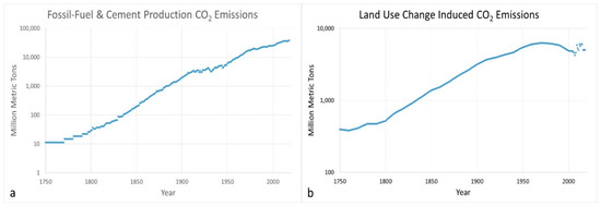
Figure 1.
(a) Global CO2 emissions into the environment from fossil fuel consumption and cement production [7,8], (b) global CO2 emissions from land-use changes [9,10].
Figure 2 displays the measurements of the CO2 concentration in the atmosphere based on the Law Dome [15] and Siple [16] ice cores and direct measurements at Mauna Loa [17,18]. The ice core data typically have temporal accuracy of ±2 years while the CO2 values for ice samples from within an annual layer were found to vary by less than 1.2 ppm [15]. For Mauna Loa, CO2 concentrations are accurate to within ±0.2 ppm [19]. These data demonstrate that the CO2 concentration has been increasing steadily since 1750 and this increase has also accelerated significantly since 1960.
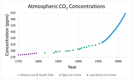
Figure 2.
Observations of atmospheric CO2 concentrations (ppm) [15,16,17,18].
Efforts to associate the change in CO2 concentration with emissions based on a variety of models have been attempted. Many of these studies examined the uptake of CO2 by the ocean as it is a large carbon sink in the environment. Examples include, study of the magnitude, variability, and trends in the global ocean carbon uptake [20], examination of feedback mechanisms and sensitivities of ocean carbon uptake under global warming [21], and reconstructions of the history of anthropogenic CO2 concentrations in oceans [22]. These studies demonstrate that the CO2 uptake by the ocean has been increasing over the past several decades and, at present, approximately 1 gram of CO2 is absorbed by the ocean for every 4 grams emitted into the atmosphere [9].
With more than one-third of the earth’s surface already altered by land-use changes (LUC) [23], it is important to consider both the past and future potential impacts of LUC on CO2 concentrations and the climate. These impacts have been the subject of several studies [24,25,26,27,28,29,30]. LUC emissions have been estimated to increase CO2 concentrations by 15–43 ppm during the time period of interest [24,25,28,29]. Bennedsen et al. [30] have performed statistical analyses to examine variations in the ocean and land sinks and the atmospheric fraction (AF). Their analysis yielded no statistical evidence that AF is varying but did find that the land sink rate was decreasing [30].
In this work, a simple semi-empirical parameterization has been developed to attempt to precisely reproduce the increase of atmospheric CO2 concentrations observed from 1751 to 2018 resulting from increase in fossil fuel and land-use change emissions of CO2 into the environment. Comparisons with observed CO2 concentrations are presented. Implications of this analysis for the terrestrial sink and the determination of AFFF are discussed.
2. Materials and Methods
This work analyzed data sets containing CO2 emissions from fossil fuel combustion [7,8,9] and land-use changes [9,10] to determine their impact upon CO2 atmospheric concentrations. This assessment included:
- An evaluation of fossil fuel and land-use change CO2 emissions with determination of best fit exponential or linear trendlines to enable comparison with prior studies, e.g., [31];
- The development of a semi-empirical model to calculate atmospheric CO2 concentrations based on the level of fossil fuel and land-use emissions;
- To compare the model results of CO2 concentration calculations using both
- o
- the traditional atmospheric fraction (AF), and,
- o
- a new approach that employs only AFFF combined with a linear component that addresses the net flux of land-based CO2 emissions combined with a rapidly varying component of the terrestrial sink;
- To determine a value for AFFF for the time period under consideration.
3. Results
3.1. Correlation of Atmospheric CO2 Concentration with CO2 Emissions
3.1.1. Traditional Approach and Discussion
The growth of carbon emissions from land-use changes [9,10,32] coupled with the burning of fossil fuels [7,8,9] is shown in Figure 3 [see Supplementary Material]. It is noted that an exponential growth curve will generally follow the overall shape of the observed data set, notwithstanding significant differences of up to 38% from the published data. It has been postulated that if the climate system is considered as a linear system forced by exponentially growing CO2 emissions, then all ratios of responses to forcings are constant [31]. In particular, AF would be constant with the value dependent upon the lifetime, τ, of the CO2 in the atmosphere [33]. A best fit to the exponential emissions growth curve yields a value of approximately 43% for AF [33].
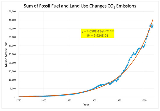
Figure 3.
Global emission levels of CO2 from fossil fuels and land-use changes; equation is best fit exponential curve to the data; R2 in each figure defines the goodness of fit.
To convert the emissions data shown in Figure 3 to changes in atmospheric CO2 concentrations, a measured base-year [2018] concentration datum of 408.52 ppm was chosen from the Mauna Loa CO2 measurements data set [17,18]. The change in the atmospheric CO2 concentration was then determined by using the combined fossil-fuel-based [7,8] and land-use changes induced CO2 emissions [9,10] for each year preceding 2018, converting those annual emission rates into an equivalent ppm of the atmosphere [mass of the atmosphere = 5.148E18 kg [34]], and then applying a single scaling factor to determine the concentration change for that year. For each year prior to 2018, the change was negative. The governing equation is:
where ATM is an atmospheric concentration in ppm, αi is the atmospheric fraction [α1 determined by best fit to be 43.1%], β = 7.782Pg of CO2 that is equivalent to 1 ppm of CO2 in the atmosphere by volume, E is CO2 emissions in million metric tons, and, N is the year. The results of the calculations [see Supplementary Material] are shown in Figure 4.
ATMN-1 = ATMN − (αi/β) x EN-1 x 10⁹
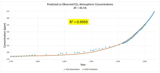
Figure 4.
Comparison of predicted CO2 concentrations with observations. Curve is best fit to data using Equation (1) with α1 = AF = 43.1%.
The fitted curve based on Equation (1) shows that the predicted concentrations follow the CO2 concentration observations reasonably well but are not a precise match. To examine this further, it is illustrative to examine the CO2 emissions more closely as a function of time to determine if an exponential growth curve assumption for emissions is warranted and hence, implying a constant value for AF. Figure 1b shows the land-use CO2 emissions [9,10]. A cursory examination of these data clearly demonstrates that the emissions do not follow an exponential growth pattern.
Now, consider fossil-fuel-based emissions in the time period from 1751 to 2018 [7,8], shown in Figure 5a. As may be seen, the agreement between the best fit exponential growth curve with the data is poor in the early 20th century and significantly worse post-1980. Although the data from the nineteenth century (Figure 5b) clearly follow an exponential growth curve (note the logarithmic scale in Figure 5b), the data post-1945 are best fit by a linear growth curve (Figure 5c).
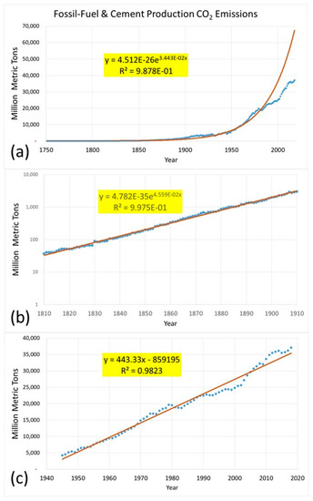
Figure 5.
(a) Comparison of best fit exponential growth curve with fossil fuel and cement production CO2 emissions (1750–2018). (b) Comparison of best fit exponential growth curve with fossil fuel and cement production CO2 emissions (1810–1910). (c) Comparison of best fit linear growth curve with fossil fuel and cement production CO2 emissions (1945–2018).
Although there is moderate agreement between the CO2 concentration observations with those predicted by Equation (1) with a fixed value of 43.1% for AF, the deviations from exponential growth of both the carbon emissions from land-use changes (Figure 1b) and from fossil fuels (Figure 5a,c) suggest that the approximate concurrence observed in Figure 3 of the sum of the emissions with an exponential growth curve is coincidental and not indicative of a fundamental physical nature of the emissions. This issue raises concerns with the postulate [31] that if the climate system is considered as a linear system forced by exponentially growing CO2 emissions, then all the ratios of responses to forcings, including AF, are constant.
It is also illustrative to consider that from 1750 to 1850, the total CO2 emissions [fossil fuel (FF) + land-use change (LUC)] equaled 71.7 Gt CO2 with 93.4% of those emissions due to land-use changes [7,8,10]. Using the conversion factor of 1 ppm of CO2 in the atmosphere by volume is equivalent to 7.782 Gtons CO2 [9], this equates to a 9.2 ppm increase of CO2 in the atmosphere if all the emitted CO2 remained in the atmosphere. The measured data [15,16] indicate a 9.8 ppm increase in CO2 atmospheric concentrations during that period. So, for 100 years at the beginning of the industrial era, this concurrence implies that ~100% of the total CO2 emissions remained in the atmosphere. This somewhat surprising result raises the question: why is there apparently no evidence of an ocean or land-based carbon sink during this century-long time span?
3.1.2. Alternative Correlation Approach
In the same manner as used to generate Figure 4, a measured base-year [2018] concentration datum of 408.52 ppm was chosen from the Mauna Loa CO2 measurements data set [17,18]. The change in the atmospheric CO2 concentration was then determined by using only the fossil-fuel-based CO2 emissions [7,8] for each year preceding 2018, converting those annual emission rates into an equivalent ppm of the atmosphere, and then applying a single scaling factor (AFFF) for each year to determine the concentration change for that year. For each year prior to 2018, the change was negative. Using Equation (1), the best fit curve to the data yields α2= AFFF = 54.5%. The results of the calculations [see Supplementary Material] are shown in Figure 6.
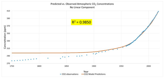
Figure 6.
Measured and predicted CO2 concentrations based on a 2018 datum base year. Curve is best fit to data using Equation (1) with scaling factor α2 = 54.5% (AFFF).
There is excellent agreement between the predicted values and experimental observations from approximately 1925 to 2018. The agreement before 1925 is less precise because the predicted values become asymptotic as the CO2 emissions from fossil fuel combustion and cement production diminish significantly during the nineteenth and eighteenth centuries while the measured atmospheric CO2 concentration values from the Siple [16] and Law Dome [15] ice cores continue a steady decline as one moves backward in time from about 1925 to 1750.
To further refine the correlation of emissions with concentration, a closer examination of the measured CO2 concentration data from 1750 to 1890 was performed. As may be seen in Figure 7, the increase in the non-fossil fuel/cement production-driven CO2 atmospheric concentration over the 140-year period is well characterized by a simple linear function. [The 1839 data point (brown triangle) was deselected from the analysis because the datum was considered out of range as its deviation from the best fit linear function was greater than 3X that of any other data point in the 1750–1890 data set.]
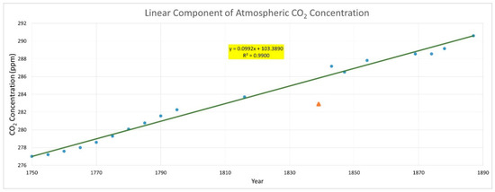
Figure 7.
Atmospheric CO2 concentrations with no fossil fuel combustion/cement production emissions inputs (Note: 1839 data point removed from analysis).
One may now characterize the overall change in atmospheric CO2 concentration since 1750 as a superposition of the linear increase shown in Figure 7 extended through the present combined with the delta induced by fossil fuel/cement production-driven CO2 emissions using an approach similar to that employed in Figure 6. The governing equation is:
where ATM is an atmospheric concentration in ppm, αi is AFFF [α3 determined by best fit to be 51.3%], β = 7.782Pg of CO2 that is equivalent to 1 ppm of CO2 in the atmosphere by volume, κ = 0.0992 is the slope of the linear component of atmospheric CO2 concentration (see Figure 7), E is fossil fuel combustion CO2 emissions in million metric tons, and N is the year. The resultant agreement to the measured data is shown in Figure 8 [see Supplementary Material].
ATMN-1 = ATMN − (αi/β) x EN-1 x 10⁹- κ
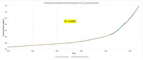
Figure 8.
Measured and predicted CO2 concentrations based on a 2018 datum base year. Curve is best fit to data using Equation (2) with scaling factor α3 = 51.3% (AFFF).
An analysis of the statistical validity of the fit of the semi-empirical model [Equation (2)] to the measured data was performed [see Supplementary Material] using Anova in Microsoft Excel [35]. A linear regression of the predicted atmospheric CO2 values versus the measured CO2 levels yields the results shown in Figure 9. The slope of 1.008 (R-square: 0.9995) demonstrates almost a perfect fit with a robust statistically significant relationship (p-value: 3.2E-140). This result provides strong statistical evidence that AFFF has been unchanged at 51.3 ± 0.4% (95% confidence interval) for the entire analysis period of 268 years.
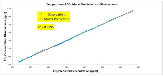
Figure 9.
Comparison of predicted CO2 atmospheric concentrations to observations.
4. Discussion
Using the terminology of Le Quéré et al. [9], the global carbon budget is a balance of emission and absorption processes. This balance equation may be written as:
where GATM is the growth rate of CO2 in the atmosphere; EFF is the estimate for CO2 emissions from fossil fuel combustion and cement production; ELUC is the estimate for CO2 emissions resulting from deliberate human activities on land; SOCEAN is the uptake of CO2 in the ocean; SLAND is the uptake of CO2 by the terrestrial sink; and, BIM is an estimate of the budget imbalance, which is a measure of the mismatch between the estimated emissions and the estimated changes in the atmosphere, land, and ocean.
GATM = EFF + ELUC − SOCEAN − SLAND + BIM
Referring to Figure 1a, one observes significant increases in fossil-fuel combustion and cement production CO2 emissions, EFF, since the mid-1700s and since 1959, emissions have increased 370% [7,8]. Models of the ocean sink, SOCEAN, have also shown increases from 5.5 ± 1.8 GtCO2 during the decade of the 1960s to 9.2±1.8 GtCO2 from 2000 to 2009 [9,20,21,22]. These emissions and ocean sink increases have generally varied smoothly over time (see Figure 3 of [9]).
ELUC has demonstrated significant interannual variability over the past two decades [9] while changes prior to 1990 have been depicted as slowly varying in the literature [9,10,32]. It is possible that the significant interannual changes since 1990 were present in ELUC pre-1990 but the estimates of the data or the models smoothed out changes from year to year. The land sink, SLAND, has also increased over the past six decades but there has been dramatic variability in CO2 absorption over short time periods estimated using either DGVMs [36,37,38,39,40,41,42,43,44,45,46] or using the residual from Equation (3) with inputs of measured and modeled EFF, ELUC, GATM, and SOCEAN [9].
To account for the significant interannual variability in the land sink, it may be hypothesized that the terrestrial carbon sink is a combination of two elements; one component that is slowly varying, SLAND SMOOTH, that responds to smooth changes in the emissions of CO2, coupled with a reactive component, SLAND REACTIVE, that responds to rapid changes in emissions and is likely correlated with the rapid changes in vegetation considered in DGVMs. This approach would enable the terrestrial sink to adapt to rapid changes in land-based emissions (and correlate with the significant variation in interannual terrestrial sink estimates) while also accounting for a fraction of the more smoothly varying fossil-fuel-based emissions.
As shown in Figure 8, it is possible to fully characterize the change in CO2 concentrations over a 268-year period using only one measured concentration datum [2018-Mauna Loa [17,18]] combined with a linear regression fit to land-use change induced CO2 concentration increases and a fixed-parameter scaled, AFFF, calculation of the changes in CO2 concentration due to fossil fuel combustion and cement production emissions prior to 2018. Based on these data, it is suggested that Equation (3) may be used to determine the net flux of land-based CO2 emissions, ELUC, combined with the reactive component of the terrestrial sink, SLAND REACTIVE, from 1750 AD to the present. As observed in Figure 7, the growth rate of GATM was constant during the selected time period, increasing approximately 0.099 ppm per year. Converting this increase to a net emissions rate, it is determined that the net flux of ELUC minus SLAND REACTIVE is 0.77 GtCO2 per year. The remainder of the land sink, SLAND SMOOTH, coupled with the ocean sink operates as a smoothly varying function that absorbs 48.7% of the emissions from fossil fuels and cement production. This somewhat non-intuitive hypothesis of two constituents comprising the terrestrial sink is borne out by the data.
Uncertainties
Each data set used in the analysis have uncertainties associated with the information. These include measurement uncertainty, uncertainty in the estimates of data, and uncertainties in the application of models to match physical measurements. For ice core data, sources of uncertainty include: timescale uncertainty that has been estimated to be ±2 years for the data included in this analysis [15,16]; sampling uncertainty, spatial uncertainty as snowfall may vary significantly over short distance; diffusion uncertainty where the characteristic length of diffusion may exceed the characteristic depth resolution proxy used in the analysis; and, uncertainties with respect to the assumptions of the relationships between variables over time [47].
EFF uncertainties are impacted by the availability of accurate and complete records for each of the pertinent quantities that input into the total value of EFF. When these are included, the total uncertainty has been estimated to range from 5% to 10% across the time range of the study [9,11,12,13]. ELUC uncertainties have been estimated to be more significant. For bookkeeping models, uncertainties range from 47% to 58% while for DGVMs they range from 32% to 50% [9].
The values for the terrestrial sink also have significant uncertainties. The residual sink uncertainties determined using Equation (3) range from 29% to 60% of the estimated SLAND values [9]. Approaches using DGVMs have uncertainties that range from 19% to 41% depending upon the selected time frame [9]. The ocean sink uncertainties range from 20% to 50% depending upon the selected decade under study. The inclusion of these uncertainties into the fitting may impact the reliability of the model to determine CO2 concentration values based on EFF and ELUC. In particular, the uncertainties noted in ELUC over the past six decades [9] imply that for a number of decades, there may have been zero emissions due to land-use change. These would call into question the validity of the linear component determined from the best fit of ELUC values that is shown in Figure 7 and hence the validity of the postulate to separate the terrestrial carbon sink into two elements. Additional research is suggested to resolve this potential issue.
5. Conclusions
A semi-empirical model has been developed to calculate CO2 concentrations from 1751 to 2018 as a function of CO2 emissions. Initial calculations using only EFF data and a constant value of AFFF = 54.5% enabled excellent replication of concentration observations from 1925 to 2018 but prior to 1925, the agreement was less precise. Predicted values become asymptotic as the EFF levels diminish significantly during the nineteenth and eighteenth centuries while the measured atmospheric CO2 concentration values continue a steady decline as one moves backward in time from about 1925 to 1750. To improve the agreement between the predicted and measured CO2 concentration values, the relationship between concentration and emissions was postulated to be a superposition of two elements. The first element with a constant concentration growth rate for the time period under consideration may be attributed to the net flux of land-use changes with a rapidly varying reactive component of the terrestrial sink. The second element is determined by a calculation using fossil-fuel combustion emissions with a single, fixed factor, AFFF, that has been determined to be unchanging over the period. It is postulated the value of AFFF is determined by a combination of the ocean sink with a smoothly varying component of the terrestrial sink. The agreement between predicted and observed CO2 concentrations is excellent across the considered time period and has determined to a strong statistical validity that AFFF has been unvarying at 51.3% for the past 268 years. If one considers the changes in factors such as emission and sequestration processes (see, e.g., Figure 1.1 from the IPCC AR5 report [32]) coupled with the non-exponential growth patterns of land-based or fossil-fuel-driven emissions negating the eigenvector approach of [31], a constant AFFF applied as in Equation (2) to fossil-fuel CO2 emissions [7,8] to accurately reproduce the changes in CO2 concentrations may be judged significant and worthy of additional study.
Supplementary Materials
The following are available online at https://www.mdpi.com/2225-1154/8/5/61/s1. The datasets generated and/or analyzed during the current study have been included with the Supplementary Materials attached to this manuscript.
Funding
This research received no external funding.
Conflicts of Interest
The author declares no conflict of interest.
References
- Fleming, J.R. Historical Perspectives on Climate Change; Oxford University Press: Oxford, UK, 1998. [Google Scholar]
- Tyndall, J. On the Absorption and Radiation of Heat by Gases and Vapours, and on the Physical Connexion of Radiation, Absorption, and Conduction. Phil. Trans. R. Soc. 1861, 151, 1–36. [Google Scholar]
- Oreskes, N. The scientific consensus on global warming. Science 2004, 306, 1686. [Google Scholar] [CrossRef] [PubMed]
- Prentice, I.C.; Farquhar, G.D.; Fasham, M.J.R.; Goulden, M.L.; Heimann, M.; Jaramillo, V.J.; Kheshgi, H.S.; LeQuéré, C.; Scholes, R.J.; Wallace, D.W.R.; et al. Climate Change 2001: The Scientific Basis. Contributions of Working Group I to the Third Assessment Report of the Intergovernmental Panel on Climate Change; Cambridge University Press: Cambridge, UK, 2001; pp. 185–237. [Google Scholar]
- Meehl, G.A.; Covey, C.; Delworth, T.; Latif, M.; Mcavaney, B.; Mitchell, J.F.B.; Stouffer, R.J.; Taylor, K.E. THE WCRP CMIP3 MULTIMODEL DATASET A New Era in Climate Change Research. BAMS 2007, 1383–1394. [Google Scholar] [CrossRef]
- Andres, R.J.; Boden, T.A.; Bréon, F.-M.; Ciais, P.; Davis, S.; Erickson, D.; Gregg, J.S.; Jacobson, A.; Marland, G.; Miller, J.; et al. A synthesis of carbon dioxide emissions from fossil-fuel combustion. Biogiosciences 2012, 9, 1845–1871. [Google Scholar] [CrossRef]
- Boden, T.A.; Andres, R.J.; Marland, G. Global, Regional, and National Fossil-Fuel CO2 Emissions; Carbon Dioxide Information Analysis Center, Oak Ridge National Laboratory, U.S. Department of Energy: Oak Ridge, TN, USA, 2013. Available online: http://cdiac.ess-dive.lbl.gov/trends/emis/overview_2010.html (accessed on 20 January 2020).
- Boden, T.A.; Marland, G.; Andres, R.J. Global, Regional, and National Fossil-Fuel CO2 Emissions; Carbon Dioxide Information Analysis Center at Appalachian State University: Boone, NC, USA, 2018; Available online: https://energy.appstate.edu/CDIAC (accessed on 20 January 2020).
- Le Quéré, C.; Robbie, A.M.; Friedlingstein, P.; Sitch, S.; Hauck, J.; Pongratz, J.; Pickers, P.A.; Korsbakken, J.I.; Peters, G.P.; Canadell, J.G.; et al. Global Carbon Budget 2018. Earth Syst. Sci. Data 2018, 10, 2141–2194. [Google Scholar] [CrossRef]
- Stocker, B.D.; Feissli, F.; Strassmann, K.M.; Spahni, R.; Joos, F. Past and future carbon fluxes from land use change, shifting cultivation and wood harvest. Tellus B Chem. Phys. Meteorol. 2014, 66, 23188. [Google Scholar] [CrossRef]
- Andres, R.J.; Fielding, D.J.; Marland, G.; Boden, T.A.; Kumar, N.; Kearney, A.T. Carbon dioxide emissions from fossil-fuel use, 1751–1950. Tellus B 1999, 51, 759–765. [Google Scholar] [CrossRef]
- Andres, R.J.; Boden, T.; Higdon, D. A new evaluation of the uncertainty associated with CDIAC estimates of fossil fuel carbon dioxide emission. Tellus B 2014, 66, 23616. [Google Scholar] [CrossRef]
- Ballantyne, A.P.; Andres, R.; Houghton, R.; Stocker, B.D.; Wanninkhof, R.; Anderegg, W.; Cooper, L.A.; DeGrandpre, M.; Tans, P.P.; Miller, J.B.; et al. Audit of the global carbon budget: Estimate errors and their impact on uptake uncertainty. Biogeosciences 2015, 2015 12, 2565–2584. [Google Scholar] [CrossRef]
- Hurtt, G.C.; Frolking, S.; Fearon, M.G.; Moore, B.; Shevliakova, E.; Malshev, S.; Pacala, S.W.; Houghton, R.A. The underpinnings of land-use history: Three centuries of global gridded land-use transitions, wood harvest activity, and resulting secondary landscapes. Glob. Chan. Biol. 2006, 12, 1208–1229. [Google Scholar] [CrossRef]
- Etheridge, D.M.; Steele, L.P.; Langenfelds, R.L.; Francey, R.J.; Barnola, J.-M.; Morgan, V.I. Historical CO2 Records from the Law Dome DE08, DE08-2, and DSS ice cores In Trends: A Compendium of Data on Global Change; Carbon Dioxide Information Analysis Center, Oak Ridge National Laboratory, U.S. Department of Energy: Oak Ridge, TN, USA, 1998. Available online: http://cdiac.ess-dive.lbl.gov/trends/co2/lawdome.html (accessed on 18 December 2019).
- Neftel, A.; Friedli, H.; Moor, E.; Lötscher, H.; Oeschger, H.; Siegenthaler, U.; Stauffer, B. Historical Carbon Dioxide Record from the Siple Station Ice Core in Trends: A Compendium of Data on Global Change; Carbon Dioxide Information Analysis Center, Oak Ridge National Laboratory, U.S. Department of Energy: Oak Ridge, TN, USA, 1994. Available online: Cdiac.ess-dive.lbl.gov/trends/co2/siple.html (accessed on 18 December 2019).
- Tans, P. 2018. Available online: http://www.esrl.noaa.gov/gmd/ccgg/trends/ (accessed on 18 December 2019).
- Keeling, R.F. 2018. Available online: scrippsco2.ucsd.edu (accessed on 18 December 2019).
- Tans, P.; Thoning, K. “How we measure background CO2 levels on Mauna Loa” NOAA ESRL Global Monitoring Division. 2018. Available online: www.esrl.noaa.gov/gmd/ccgg/about/co2_measurements.html (accessed on 5 January 2020).
- Wanninkhof, R.; Park, G.-H.; Takahasi, T.; Sweeney, C.; Reely, R.; Nojiri, Y.; Gruber, N.; Doney, S.C.; McKinley, G.A.; Lenton, A.; et al. Global ocean carbon uptake: Magnitude, variability and trends. Biogeosciences 2013, 10, 1983–2000. [Google Scholar] [CrossRef]
- Plattner, G.-K.; Joos, F.; Stocker, T.F.; Marchal, O. Feedback mechanisms and sensitivities of ocean carbon uptake under global warming. Tellus B Chem. Phys. Meteorol. 2001, 53, 564–592. [Google Scholar] [CrossRef][Green Version]
- Khatiwala, S.; Primeau, F.; Hall, T. Reconstruction of the history of anthropogenic CO2 concentrations in the ocean. Nature 2009, 462, 346–349. [Google Scholar] [CrossRef] [PubMed]
- Boysen, L.R.; Brovkin, V.; Arora, V.K.; Cadule, P.; de Noblet-Ducoudré, N.; Kato, E.; Pongratz, J.; Gayler, V. Global and regional effects of land-use change on climate in 21st century simulations with interactive carbon cycle. Earth Syst. Dyn. 2014, 5, 309–319. [Google Scholar] [CrossRef]
- Matthews, H.; Weaver, A.; Meissner, K.; Gillett, N.; Eby, M. Natural and anthropogenic climate change: Incorporating historical land cover change, vegetation dynamics and the global carbon cycle. Clim. Dyn. 2004, 22, 461–479. [Google Scholar] [CrossRef]
- Brovkin, V.; Sitch, S.; von Bloh, W.; Claussen, M.; Bauer, E.; Cramer, W. Role of land cover changes for atmospheric CO2 increase and climate change during the last 150 years. Glob. Change. Biol. 2004, 10, 1253–1266. [Google Scholar] [CrossRef]
- Brovkin, V.; Boysen, L.; Arora, V.; Boisier, J.; Cadule, P.; Chini, L.; Claussen, M.; Friedlingstein, P.; Gayler, V.; van den Hurk, B.J.J.M.; et al. Effect of anthropogenic land-use and land cover changes on climate and land carbon storage in CMIP5 projections for the 21st century. J. Clim. 2013, 26, 6859–6881. [Google Scholar] [CrossRef]
- Sitch, S.; Brovkin, V.; von Bloh, W.; van Vuuren, D.; Eickhout, B.; Ganopolski, A. Impacts of future land cover changes on atmospheric CO2 and climate. Glob. Biogeochem. Cycles 2005, 19, GB2013. [Google Scholar] [CrossRef]
- Shevliakova, E.; Stouffer, R.J.; Malyshev, S.; Krasting, J.P.; Hurtt, G.C.; Pacala, S.W. Historical warming reduced due to enhance land carbon uptake. Proc. Natl. Acad. Sci. USA 2013, 110, 16730–16735. [Google Scholar] [CrossRef]
- Pongratz, J.; Reick, C.; Raddatz, T.; Claussen, M. Biogeophysical vs. biogeochemical climate response to historical anthropogenic land cover change. Geophy. Res. Lett. 2010, 37, L08072. [Google Scholar] [CrossRef]
- Bennedsen, M.; Hillebrand, E.; Koopman, S.J. Trend analysis of the airborne fraction and sink rate of anthropogenically released CO2. Biogeosciences 2019, 16, 3651–3663. [Google Scholar] [CrossRef]
- Raupach, M.R.; Canadell, J.G.; LeQuéré, C. Anthropogenic and biophysical contributions to increasing atmospheric CO2 growth rate and airborne fraction. Biogeosciences 2008, 5, 1601–1613. [Google Scholar] [CrossRef]
- Stocker, T.F.; Qin, D.; Plattner, G.-K.; Tignor, M.; Allen, S.K.; Boschung, J.; Nauels, A.; Xia, Y.; Bex, V.; Midgley, P.M. Climate Change 2013: The Physical Science Basis. Contribution of Working Group I to the Fifth Assessment Report of IPCC the Intergovernmental Panel on Climate Change; Cambridge University Press: Cambridge, UK; New York, NY, USA, 2013. [Google Scholar]
- Terenzi, F.; Khatiwala, S. Modeling the atmospheric airborne fraction in a simple carbon cycle model. Tellus B 2009, submitted. [Google Scholar]
- Trenberth, K.E.; Smith, L. The Mass of the Atmosphere: A Constraint on Global Analyses. J. Clim. 2005, 18, 864–875. [Google Scholar] [CrossRef]
- Microsoft Corporation. Microsoft Excel. 2018. Available online: https://office.microsoft.com/excel (accessed on 12 February 2020).
- Lawrence, D.M.; Oleson, K.W.; Flanner, M.G.; Thornton, P.E.; Swenson, S.C.; Lawrence, P.J.; Zeng, X.; Yang, Z.-L.; Levis, S.; Sakaguchi, K.; et al. Parameterization improvements and functional and structural advances in version 4 of the Community Land Model. J. Adv. Model. Earth Syst. 2011, 3, M03001. [Google Scholar] [CrossRef]
- Levy, P.E.; Cannell, M.G.R.; Friend, A.D. Modelling the impact of future changes in climate, CO2 concentration and land use on natural ecosystems and the terrestrial carbon sink. Glob. Environ. Chang. 2004, 14, 21–30. [Google Scholar] [CrossRef]
- Clark, D.B.; Mercado, L.M.; Sitch, S.; Jones, C.D.; Gedney, N.; Best, M.J.; Pryor, M.; Rooney, G.G.; Essery, R.L.H.; Blyth, E.; et al. The Joint UK Land Environment Simulator (JULES), model description – Part 2: Carbon fluxes and vegetation dynamics. Geosci. Model Dev. 2011, 4, 701–722. [Google Scholar] [CrossRef]
- Cox, P.M. Description of the “TRIFFID” Dynamic Global Vegetation Model; Hadley Centre: Exeter, UK, 2001. Technical Note 24 2001.
- Sitch, S.; Smith, B.; Prentice, I.C.; Arneth, A.; Bondeau, A.; Cramer, W.; Kaplan, J.O.; Levis, S.; Lucht, W.; Sykes, M.T.; et al. Evaluation of ecosystem dynamics, plant geography and terrestrial carbon cycling in the LPJ dynamic global vegetation model. Glob. Change. Biol. 2003, 9, 161–185. [Google Scholar] [CrossRef]
- Smith, B.; Prentice, I.C.; Sykes, M.T. Representation of vegetation dynamics in the modelling of terrestrial ecosystems: Comparing two contrasting approaches within European climate space. Glob. Ecol. Biogeogr. 2001, 10, 621–637. [Google Scholar] [CrossRef]
- Ahlström, A.; Miller, P.A.; Smith, B. Too early to infer a global NPP decline since 2000. Geophys. Res. Lett. 2012, 39, L15403. [Google Scholar] [CrossRef]
- Zaehle, S.; Ciais, P.; Friend, A.D.; Prieur, V. Carbon benefits of anthropogenic reactive nitrogen offset by nitrous oxide emissions. Nat. Geosci. 2011, 4, 601–605. [Google Scholar] [CrossRef]
- Krinner, G.; Viovy, N.; de Noblet-Ducoudré, N.; Ogee, J.; Polcher, J.; Friedlingstein, P.; Ciais, P.; Sitch, S.; Prentice, I.C. A dynamic global vegetation model for studies of the coupled atmosphere-biosphere system. Glob. Biogeochem. Cycles 2005, 19, Gb1015. [Google Scholar] [CrossRef]
- Woodward, F.I.; Lomas, M.R. Vegetation dynamics—Simulating responses to climatic change. Biol. Rev. 2004, 79, 643–670. [Google Scholar] [CrossRef]
- Zeng, N.; Mariotti, A.; Wetzel, P. Terrestrial mechanisms of interannual CO2 variability. Glob. Biogeochem. Cycles 2005, 19, GB1016. [Google Scholar] [CrossRef]
- Steig, E.J. Sources of Uncertainty in Ice Core Data. In White paper from Workshop on Reducing and Representing Uncertainties in High-Resolution Proxy Data; PAGES/CLIVAR Proxy Uncertainty Workshop: Trieste, Italy, 2008. [Google Scholar]
© 2020 by the author. Licensee MDPI, Basel, Switzerland. This article is an open access article distributed under the terms and conditions of the Creative Commons Attribution (CC BY) license (http://creativecommons.org/licenses/by/4.0/).