
Investigating Planar and Nonplanar Wing Planform Optimisation for Ground Effect Aircraft

Engineering Mechanics, KTH Royal Institute of Technology, SE-100 44 Stockholm, Sweden
*
Author to whom correspondence should be addressed.
†
These authors contributed equally to this work.
Aerospace 2023, 10(11), 969; https://doi.org/10.3390/aerospace10110969
Submission received: 18 September 2023
/
Revised: 7 November 2023
/
Accepted: 14 November 2023
/
Published: 17 November 2023
(This article belongs to the Section Aeronautics)
Abstract
:Wing-in-Ground (WIG) effect aircraft are gaining attention for their potential in reducing environmental impact. However, optimising wing planforms based solely on aerodynamics might improve performance while compromising static height stability of WIG aircraft. This study investigates the effects of planar and nonplanar wing planform optimisation for regional transport ground effect aircraft. Three distinct multiobjective wing planform optimisations are explored: planar wing optimisation, nonplanar wing optimisation, and nonplanar wingtip optimisation. These optimisations assess the impact on both aerodynamic efficiency and static height stability characteristics of a wing planform in ground effect, at three different flying altitudes. In extreme ground effect, the Pareto set includes wings with negative spanwise camber, enhancing both cushion sensation and aerodynamic efficiency by effectively utilizing ground effect, thus proving advantageous over planar wing configurations.
1. Introduction
Aviation industry is entering a new era with great interest in developing revolutionary aircraft technology to meet the strict regulations for reducing CO and NO emissions by 2050 [1]. This opens up opportunities to look back at aircraft concepts that showed great potential in terms of efficiency and were abandoned due to lack of technological progress. One such concept is the Wing-in-Ground effect (WIG) aircraft, which operates close to the ground and leverages the ground effect to achieve improved efficiency [2]. When an aircraft is flying close to the ground, the presence of ground limits the vertical extent to which the wingtip vortices can expand. Consequently, these vortices extend horizontally or spanwise along the ground surface, effectively increasing the spanwise length of the wake. This leads to an increase in the effective aspect ratio of the wing, causing it to behave as if it has a longer wingspan. As a result, there is a reduction in the induced drag, thus improving aerodynamic efficiency represented by the lift-to-drag ratio. Furthermore, the ground effect phenomenon shifts the stagnation point to the lower surface of the wing, redirecting a significant portion of incoming airflow over the upper surface of the wing [3]. This change in airflow reduces the airspeed beneath the wing, leading to an increase in air pressure, effectively creating an air cushion. This cushion sensation can be quantified by calculating the derivative of the lift coefficient with respect to the flying altitude. When WIG aircraft are designed to operate at relatively low altitudes, this air cushion generates an additional lift component known as “RAM” pressure. This contributes significantly to the overall efficiency of the aircraft, enabling them to carry heavier payloads or travel longer distances with the same fuel capacity compared to traditional aircraft flying at higher altitudes.
One of the primary challenges in designing and operating WIG aircraft is to maintain static stability during cruise conditions. Unlike conventional aircraft operating out of ground effect, the presence of gusts can induce changes in both the pitch angle and flying altitude of WIG aircraft. Consequently, WIG aircraft should be capable of autonomously returning to their original pitch angle and flying altitude without requiring active correction by the pilot. Therefore, a WIG aircraft is required to have static stability in pitch and static stability in height (vertical direction) [2]. Researchers have proposed various design solutions to improve the static stability of WIG aircraft. For example, the third-generation Ekranoplan series from Russia utilized a rectangular wing design with a large horizontal tailplane outside the ground effect, which improved static stability but increased Maximum Take-Off Weight (MTOW) and take-off power requirements [4]. Alternatively, Lippich suggested a reverse delta wing design with an anhedral angle for the X-112 and X-114 models which improved inherent static stability of a wing planform and reduced the size of the horizontal tail unit [5]. Recently AirFish-8 WIG aircraft utilized Lippich-type wing planform for 8–10 seater configuration. However, the effectiveness of this design on a regional transport WIG aircraft remains unproven, as it was only tested on small aircraft with a capacity of upto 10 passengers.
Staufenbiel and Schlichting [6] emphasized the significance of wing design in achieving longitudinal static height stability for WIG aircraft. They proposed a static height stability criterion, which solely relies on the ground effect factors that quantify the changes in aerodynamic coefficients resulting from the ground effect phenomenon. More specifically, the change in lift coefficient with respect to flying altitude of a wing plays a significant role in maintaining the static height stability requirements of a WIG aircraft. Thus, shifting the CG location of a WIG aircraft is insufficient in achieving static stability in height. More recently, Fevralskikh [7] proposed a RANS-based simulation approach to perform longitudinal static height stability analysis of a WIG aircraft in cruise condition. Chang et al. [8] conducted a wind tunnel experiment to examine the static and dynamic stability of a 20-passenger WIG aircraft and showed the need for a large tail unit to improve static stability and damping ratio for short-period pitching oscillations. Kornev and Matveev [9] analyzed the dynamic motion of a WIG aircraft using numerical methods in both normal and critical conditions and recommended strategies for safety during maneuvering and transition modes. Their findings emphasized the importance of inherent stability characteristics of a wing design to minimise pilot intervention. Thus, it is essential to optimise wing design by increasing the aerodynamic efficiency and minimising the tendency to variation in pitch attitude due to external turbulence in close proximity to the ground. By enhancing the inherent static stability characteristics of a wing design, the reliance on large tail units and advanced control systems can be reduced, leading to improved aircraft performance and decreased MTOW of a WIG aircraft.
Over the years, several studies have focused on multi-objective optimisation of airfoil shapes to improve both aerodynamic efficiency and static height stability characteristics of a WIG aircraft [10,11,12]. Results highlight the significant influence of S-shaped camber line on the lift-based ground effect factor, which plays a crucial role in enhancing the static height stability characteristics and overall aerodynamic efficiency of airfoils operating in ground effect conditions. It is important to note that ground effect is a three-dimensional phenomenon, hence its benefits cannot be fully explored through two-dimensional airfoil optimisation alone. Nonplanar wings have been shown to reduce the induced drag beyond planar wings [13,14]. However, only few examples are available in the literature to better understand whether nonplanar wings could satisfy the stability requirements of WIG aircraft. Kim et al. [15] utilized vortex lattice method (VLM) to obtain optimum configuration for medium sized ground effect aircraft with constraints on the longitudinal static height stability requirements. Studies conducted by J. Lee et al. [16] and T. Lee et al. [17] have examined the static height stability and aerodynamic characteristics of nonplanar wings in ground effect. S. Lee et al. [18] performed three dimensional wing optimisation by considering lift coefficient, aerodynamic efficiency and static height stability condition as objectives. Even though the design shows better performance, the considered planform parameterisation is not sufficient to generate large planform variations in optimisation, thus affecting the optimal solution.
Although high-fidelity gradient-based aerodynamic optimisation has significantly matured over the past two decades [13,19,20], its optimal application remains within the detailed design stage, particularly when starting with solutions already close to the optimum. On the other hand, recent years have seen advancements in low-fidelity rapid simulation tools aimed for aerodynamic shape optimisation of wings. Jansen et al. [21] utilized a panel method to compute induced drag and drag polar data for predicting viscous drag on nonplanar lifting surfaces. In a numerical optimisation study on winglets, Ning and Kroo [22] employed a vortex-lattice method to calculate induced drag while assuming a parabolic relationship between viscous drag and lift. Smith et al. [23] applied panel methods for optimising wing planforms by minimizing the induced drag and then extended the approach to incorporate non-planar variations in the design space and coupled it with XFOIL for viscous drag computation [14]. Recently, Salem et al. [24] employed a VLM method to include ground effect aerodynamics in the assessment of take-off considerations within the conceptual design of box-wing aircraft.
When coupled with the method of images, aerodynamic characteristics in ground effect can be rapidly computed using the low-fidelity simulation tools. This approach provides a distinct advantage by allowing the integration of conflicting objectives and stability derivatives during the initial design phase. Furthermore, when coupled with gradient-free optimisers, these tools enable designers to efficiently navigate the design space and strike a balance between aerodynamics and longitudinal static height stability requirements of a WIG aircraft in a single optimisation run. This approach allows them to gain a comprehensive understanding of unconventional technologies, such as ground effect aircraft, especially during the early design stage, where the lack of a design database can limit the design maturity.
The wing planform significantly influences the cushion effect of WIG aircraft by impacting the ground effect phenomenon. By appropriate selection of wing shape and its planform parameters, it becomes possible to enhance ground effect utilization and potentially decrease the reliance on large tail units for maintaining required longitudinal static height stability margin [2]. However, the integration of both aerodynamics and longitudinal static height stability characteristics into a wing planform design for ground effect applications has not been adequately explored. Therefore in this study, a multi-objective planar and nonplanar wing planform optimisation is performed to identify a range of planform shapes that have the potential to enhance both aerodynamic efficiency and cushion sensation while satisfying lift coefficient and geometry requirements. In optimising wing planforms for ground effect aircraft, two key approaches can be employed: fixing the flying altitude [25] or fixing the non-dimensional altitude (), which is the ratio between the flying altitude and wing span . It is essential to note that aircraft experience the ground effect when they fly within one wing span of the ground or other surfaces. Therefore, optimising a wing planform by fixing the non-dimensional altitude allows for a comprehensive exploration of various trends making it more suitable for uncovering generalized solutions that can apply across a range of altitudes and ground effect zones. In this work, optimisation is performed by fixing the non-dimensional altitude, termed as the design height ratio . Furthermore, the study investigates how changes in the height ratio influence the optimal wing designs. To explore this, a series of wing planform optimisations are conducted at three distinct height ratios, starting from , which is at the border of the ground effect zone, and progressing to and , representing the extreme ground effect zone. The consideration of aerodynamics and static stability computations is performed by using the rapid low-fidelity solver VSPAERO. The wing planform is parameterised using OpenVSP [26], and a multi-objective evolutionary algorithm is employed to drive the optimisation process.
The paper is structured as follows: In Section 2, physics models are discussed, which include the VLM method with the method of images, profile drag computation and brief overview of the longitudinal static stability of a WIG aircraft. Section 3 cover the baseline configuration and wing planform parameterisation. Section 4 introduces the formulation of the optimisation problem, which includes the optimisation framework, a mesh convergence study, and a brief overview of the optimisers used in this work. In Section 5, results and discussion are presented, followed by conclusions in the final section.
2. Physics Models
2.1. Vortex Lattice Method
In this work, the open-source aerodynamic analysis solver VSPAERO, is utilized to predict the aerodynamic coefficients of a lifting wing. VSPAERO offers two potential flow techniques: the panel method and the vortex lattice method (VLM) [26]. In this work, VLM method is used to compute aerodynamic loads along the span, coefficient of lift , stability derivatives term and induced drag coefficient . In the VLM method, camber surface of the wing is treated as the lifting surface and is discretized into a series of quadrilateral panels both in the chordwise and spanwise directions, each with a different orientation to account for the changing camber and twist along the span. Figure 1 illustrates the wing and its panel discretization of the cambered surface.
Vortex rings of unknown strength are placed on each panel, with the leading segment of each vortex ring positioned on the panels quarter-chord line. The governing equation for the VLM method represents that the normal velocity across the cambered surface is zero, which is evaluated at the control point on each panel, positioned at the center of the three-quarter chord line. This equation can be expressed as:
where A is the aerodynamic influence coefficient matrix. The element of A is where is the induced velocity on panel ‘i’ due to the vortex on panel ‘j’, is the normal vector computed at each panel which includes the local nonplanar geometry information. represents the strength of the vortex rings and b is a column vector which depends on freestream velocity, angle of attack and the side slip angle which is kept at zero in this work. For further details on VLM methods, readers are encouraged to refer to Katz and Plotkin [27]. Once is known, the Trefftz plane integration method is utilized to calculate the aerodynamic forces. When compared with surface pressure integration this method is less susceptible to discretization errors [28]. Using the Trefftz plane analysis, the lift and the induced drag are calculated using the following definitions, with derivations available in Drela (2014) [29]:
Here, represents the number of wake panels, is the density of the freestream flow, and denote the vortex strength and induced velocity at the mid point of the jth wake panel. Additionally, and represent the orientation and length of the jth wake panel in the Trefftz plane as shown in Figure 2. The accuracy of the VLM method within VSPAERO for calculating subsonic aerodynamic quantities has been demonstrated in the author’s previous work [25]. Due to its simplicity and low computational cost, the VLM method has gained increased applicability and is widely used in other open-source tools such as Athena Vortex Lattice (AVL) [30] and OpenAeroStruct for aerostructural analysis and optimization [31].
2.2. Method of Images
The method of images is a widely recognized approach that can be integrated with any potential flow algorithm to predict aerodynamic coefficients of a lifting wing in ground effect [29]. In VSPAERO, the wing is initially set to the desired angle of attack , and a mirrored set of panels is created on the imaginary wing which is positioned at a distance 2H from the center of gravity of the main wing, as shown in Figure 3. This effectively simulates the reflection of the real wing across the plane of reflection. Each panel on the real wing corresponds to an associated image panel. The aerodynamic influence matrix A now incorporates the influence of both the real and image panels on each control point, and represents the vector of vortex strengths (circulations) for all panels, including both real and image panels . By combining the flow around the main wing with its mirror image, the downwash generated by the main wing is precisely counteracted by the upwash generated by its mirror image, resulting in a net zero flow normal to the plane of symmetry. This effectively represents a solid and flat ground. For this study, optimisation is conducted under the assumption of WIG aircraft operation above a calm sea. As a result, the influence of surface waviness on calculated aerodynamic coefficients is not taken into consideration.
2.3. Profile Drag
VSPAERO estimates the profile drag coefficient of a lifting surface using a quadratic function derived from an empirical fit of NACA 0012 airfoil data. This estimation is not valid for airfoils that exhibit a drag bucket behavior in the drag polar, such as natural laminar flow airfoils and NACA six series airfoils. Moreover, for thick airfoils, the approximation underpredicts the overall drag and cannot provide the required accuracy. Therefore, in this work, a hybrid aerodynamic formulation is employed by combining a linear 3D potential code VSPAERO with 2D sectional viscous data computed using higher order panel method with integral boundary layer formulations available in XFOIL [32]. Wing surface is first divided into a number of strips , and each strip is treated as a separate component. For each spanwise strip, 2D cross-sectional shapes are taken from the mid region. Reynolds number is calculated using the local flow conditions taken from VSPAERO within the airfoil plane and the chord length at each wing section. Profile drag coefficients are then computed using XFOIL by matching the local sectional lift coefficients calculated from VSPAERO.
In this work, a single point optimisation approach is employed to optimise the wing planform specifically for the cruise condition. The lift coefficient is constrained to a value of 0.5 and the angle of attack is varied within the linear region. Therefore it can be reasonably assumed that the impact of ground effect on skin frictional drag and pressure drag is negligible compared to induced drag, so the ground effect is not included in the profile drag calculation. The flight conditions of the wing at sea level are considered with Mach . The total profile drag coefficient, can be obtained by summing the contributions over all the sections. For half wing model, the profile drag coefficient can be written as,
where is the total number of strips, q is the dynamic pressure, S is the wing planform area, and is the profile drag and area of the ith strip respectively. Then, the total drag coefficient for the full model including both left and right wings can be expressed as [33],
2.4. Longitudinal Static Stability
Given its low altitude above the ground, a WIG aircraft is prone to turbulence generated by the surface, resulting in variations in both pitch angle and flying altitude. Therefore, a WIG craft should satisfy longitudinal static stability in both pitch and height. The longitudinal static stability of a WIG aircraft can be assessed by computing the derivative of the lift and moment coefficients with respect to the angle of attack and height and can be defined as:
where H represents the distance between the center of gravity of a wing planform and the ground surface, is the mean aerodynamic chord. Here and represents coefficient of lift and moment computed in ground effect. The derivatives of aerodynamic coefficients with respect to height are known as ground effect factors.
2.4.1. Pitch Attitude
Once the stability derivatives are computed , pitch attitude of a WIG aircraft can be determined from the equations of WIG equilibrium as presented by [9]. The pitch attitude represents how the pitch angle and flying altitude are affected by changes in the vehicle speed , which can be written as,
A stable WIG aircraft should have the minimum tendency to change the pitch attitude so as to fly steadily without active correction by the pilot which reduces the workload on the pilot and improves overall flight safety.
2.4.2. Static Stability in Pitch
The necessary criteria for longitudinal static stability in pitch are
where is the residual pitching moment when the lift force is zero [34]. In terms of netural point, Equation (10) can be written as,
The distance between the netural point and the center of gravity normalized by the mean aerodynamic chord is defined as “Static Margin in Pitch” which should be positive to achieve longitudinal static stability in pitch. Hence position of the center of gravity should be maintained before the neutral point. Static stability condition in pitch is completely general and applicable to any aircraft.
2.4.3. Static Stability in Height
Static stability condition in height according to Staufenbiel and Schlichting [6] can be written as,
Using the concept of derivatives, the influence of ground on the pitching moment coefficient can be included to Equation (12),
Equations (13) and (14) can be combined and rearranged as,
Thus the stability condition given in Equation (12) can be rewritten as,
where is the moment ratio. Equation (12) represents the ground effect condition, where a stable WIG aircraft is expected to increase lift as it reduces flight altitude. Conversely, a decrease in lift can occur when reducing flight altitude, primarily due to the Venturi effect, which causes a localized increase in airspeed beneath the wing [18]. This can result in a decrease in air pressure and the potential disruption of the air cushion. Therefore, the Venturi effect can lead to static instability in height, affecting the aircraft’s lift and pitch attitude as given in Equation (8). Equation (12) highlights the significance of the lift-based ground effect factor , which quantifies the aircraft’s cushioning effect and it is influenced by the shape of the passage formed between the lower wing surface and the ground. The configuration of this passage can be parallel, convergent, divergent, or a combination of these, as detailed in [35]. Assuming a flat ground surface, the passage’s specific shape depends on various factors, including flying altitude, wing planform parameters, angle of attack, and the shape of the lower wing surface.
In close proximity to the ground, the term is negative, providing a stabilizing influence. Conversely, for a statically stable aircraft , the moment ratio is negative and introduces destabilizing effects in Equation (16), heavily depends on . To achieve the required static margin, the magnitude of depends on factors such as tail volume ratio and tail efficiency . Consequently, a large horizontal tail unit is necessary to mitigate the adverse impact of the moment ratio term. However, the absolute value of is depends on flying altitude, airfoil shape, and wing planform shape [6]. During cruise conditions, the main wing operates in ground effect, thus significantly influencing the cushioning effect of a WIG aircraft. Designing a wing planform with a more negative value enhances the cushion effect and augments inherent static height stability characteristics, thereby enabling the use of a smaller tail unit to satisfy static pitch and height stability requirements.
3. Baseline Design and Case Definition
3.1. Baseline Design
In this study, design requirements suitable for a regional transport ground effect vehicle are utilized as baseline. To establish a baseline model, the conventional tube and wing configuration of the ATR 42-600, a high-wing, twin turboprop regional aircraft is utilized. It is important to note that, this aircraft is not intended for ground effect applications and is only used as a reference case. The CAD model of the baseline wing planform together with fuselage and tail unit is shown in Figure 4 and summary of the design is shown in Table 1 [36,37].
The shape of the airfoil plays a significant role in both the aerodynamic performance and pitch attitude of the wing. Although reflex airfoils have been proposed to minimise pitch sensitivity, they may have lower maximum lift coefficients than conventional airfoils [11]. This may not be ideal for a regional transport WIG aircraft that requires high lift at low speeds. Therefore, in this study, a baseline wing planform is designed with NACA 63 series airfoil, which is known for its high lift and low drag characteristics hence suitable for ground effect vehicles. The NACA 63418 airfoil is chosen for the root section, providing a larger thickness-to-chord ratio to withstand the higher loads near the fuselage attachment point [37]. Along the span, the thickness-to-chord ratio decreases linearly, reaching at the wing tip. The cross-sectional shape of the airfoil remains unchanged throughout the design process hence thickness-to-chord ratio of the wing sections is not altered during optimisation.
3.2. Geometry Parameterisation Using OpenVSP
In this study, OpenVSP geometry tool is used to parameterise the wing planform and handle surface mesh deformations in the design process. OpenVSP (Vehicle Sketch Pad) is an open source parametric computer-aided design (CAD) tool that is specifically designed for the conceptual design of aircraft [26]. It allows for rapid parameterisation of geometries at various levels, including planform alterations and local surface changes using the CST parameterisation method [38]. One of its unique features is the blending tool that allows for smooth transitions between different shapes or sections of a design, particularly for wing and blended wing body configurations. The blending tool uses NURBS curve to define the shape of the blend between root and tip section of a wing segment and has several parameters that can be adjusted to control the shape of the blending curve including the strength parameter , which is considered in this study. The strength parameter determines how quickly the transition occurs between two sections. This effect is shown in Figure 5, which showcases the impact of the strength parameter on the inboard segment of the wing. A higher strength value results in a more gradual transition, while a lower strength value leads to a more abrupt transition. Incorporating the blending tool within the design process ensures smoothness along the spanwise direction, negating the need for additional constraint handling procedures. The ATR 42-600 model shown in Figure 4 is designed using OpenVSP. To investigate the impact of planar and nonplanar wing configurations for ground effect applications, the wing planform is parameterised using the following three different cases.
3.2.1. Case-1: Planar Optimisation
In this case, the wing planform geometry is parameterised using a single wing segment and described by four design parameters: wing span , root chord , tip chord , and twist . In each wing segment, OpenVSP defines twist angle as a combination of two variables, one at the root and another at the tip. However, in this work, the twist angle at the root of a wing segment is held constant, and only the twist angle at the tip is considered as design variable. Sweep angle and dihedral angle are not considered as design variables, and only planar deformations are taken into account. Additionally, the blend strength parameter at the root section is also taken as a design variable which enables the optimiser to achieve a wide range of blend shapes, from gentle curves to sharp corners similar to a trapezoidal wing planform.
3.2.2. Case-2: Nonplanar Wing Optimisation
In this case, the wing design is divided into two segments using the blending tool. The inner wing segment is defined by three design variables: root chord , tip chord , and twist . Whereas, the outer wing segment is defined using three design variables: tip chord , twist , and dihedral angle . Similar to Case-1, the twist angle at the tip of each wing segment is taken as the design variable. The wing sweep angle is not considered as a design variable and is set to zero degrees throughout the optimisation. The total curve length of the wing is considered as design variable, with curve length of the inner and outer segments maintaining 40% and 60% of the total curve length, respectively. In OpenVSP, the span of the wing can be defined using two different approaches: the projected wing span and the span based on total curve length. The projected span is a simplified representation that essentially projects the wing onto a two-dimensional plane. On the other hand, the total curve length span takes into account the actual shape of the wing, including any variations in spanwise camber. However, it’s worth noting that when calculating aspect ratio, the projected wing span is used as this is the standard definition.
The dihedral angle of the outer wing segment is included as a design variable to account for nonplanar geometries. Blending strength parameter of the inner wing segment is also considered as a design variable. Segment continuity is maintained by aligning the tip chord of the inner segment with the root chord of the outer wing segment . To maintain continuity at the transition region, smoothness of the LE and TE region is set to align with the inboard and outboard region.
3.2.3. Case-3: Nonplanar Wingtip Optimisation
In this case, the focus is on optimising the wingtip design for ground effect conditions. The baseline wing is divided into two segments and parameterised using a blending tool, with design variables similar to Case-2. However, in this case the curve length of the outer wing segment is reduced to 30% of the total curve length and both dihedral angle and sweep angle of the last 30% of the wing are also used as design variables. Figure 6 shows the definition of planform design variables considered in each case. It is important to note that the blending strength parameter of the outer wing segment is not taken as a design variable in both Case-2 and Case-3 hence the blending strength influence is restricted within the wing root. As a result, the design space offered by each parameterisation is different which can allow the optimiser to explore a wide range of design configurations in each case.
4. Optimisation Problem Formulation and Framework
By integrating aerodynamics and longitudinal static height stability characteristics in a wing planform optimisation, the aim is to generate an optimised wing planform database across a range of operating height ratios. This facilitates the identification of important wing planform parameters for further investigation.
4.1. Optimisation Problem Formulation
This study explores two main objective functions: minimising the drag coefficient and the ground effect factor which measures the change in lift coefficient with respect to change in flying altitude. While reducing the drag coefficient is essential for enhancing aerodynamic efficiency of the aircraft, minimising the lift-based ground effect factor plays a crucial role in enhancing longitudinal static height stability characteristics of a wing planform. The study optimises the wing planform at a design cruise speed of 100 knots with a constrained cruise lift coefficient of . Additionally, the optimisation is performed at three different height ratios to explore how different wing parameterisations affect optimal solutions at various height ratios, where H is the distance (flying altitude) measured from the ground to the wing center of gravity (CG). The objective functions considered in this study are conflicting with each other. Therefore, additional inequality constraints have been introduced to ensure that the total drag coefficient and ground effect factor of the optimised wing planform geometries do not exceed the reference values calculated using the baseline ATR 42-600 wing planform at each height ratio in ground effect conditions. These constraints narrow down the search space and prevent solutions from favoring improvement in one objective function at the expense of the other. The mathematical formulation of the three-dimensional wing planform optimisation with constraints is defined accordingly.
where represents the vector of design variables with lower and upper bounds and respectively. , represents the design variable vector for each optimisation case. In all the cases, angle of attack of the wing is also taken as design variable, is the design lift coefficient, S represents the planform area, is the planform area which corresponds to the baseline design. and represent the total drag coefficient and ground effect factor of the baseline geometry computed in ground effect condition respectively. The number of design variables varies among the three cases, with Case-1 having 6 design variables, Case-2 having 9 design variables, and Case-3 having 10 design variables. Table 2 provides details of the design variables and their corresponding boundaries for each case based on the ATR 42-600 baseline geometry. Lower and upper bounds are chosen to allow for significant planform change but somewhat realistic. The root and tip chords of the inner wing segment of the baseline geometry are denoted as and , respectively, while the root and tip chords of the outer wing segment are denoted as and and represents the wing span. Furthermore, constraints have been placed on wing loading to ensure that the wing area is adequate to achieve the desired cruise design lift coefficient. Specifically, we assume a maximum take-off weight (MTOW) of 35,000 lbs and impose an upper limit of 100 lb/ft and a lower limit of 60 lb/ft on wing loading. These limits serve to define the acceptable range for the wing planform area, which is based on the reference wing design chosen for this study. These constraints on the wing loading have been chosen based on prevalent trends in the regional turboprop market (out-of-ground effect) observed over the past two decades [36,39]. The problem formulation presented in Equation (17) is designed to explore the impact of wing planform parameters on aerodynamics and longitudinal static height stability characteristics in different ground effect zones. In practical design studies, it might be necessary to include additional constraints related to structural weight and directional stability requirements.
4.2. Mesh Convergence Study
To demonstrate the accuracy of the mesh utilized in the optimisation process, a mesh convergence study was conducted. Nine levels of grid were created with varying numbers of panels distributed along the chordwise and spanwise directions. Figure 7 shows the convergence of relative errors for , , and in relation to the total number of panels. This grid refinement study was performed using Case-1 wing parameterisation at a 3-degree angle of attack for two different height ratios . For all the optimisation problems presented in this study, grid level L5 with a chordwise discretisation of 100 panels and a spanwise discretisation of 50 panels, was chosen since its relative error was below 1% as shown in Figure 7. The difference between the two mesh levels L1 and L5, on the camber surface with two different values of the blending strength parameter of the inner wing segment obtained using Case-3 wing parameterization is illustrated in Figure 8. A higher strength value results in a more gradual variation of chord, while a lower strength value resuls in a linear variation of chord along the spanwise direction. A close view of the paneling in the tip region is also shown in Figure 8. This clearly indicates that spanwise camber of the wing is significantly influenced by the spanwise panel density and mesh level L5 is sufficient for accurately modeling the spanwise camber and curvature of the wing along its entire span.
4.3. Optimiser
In a multi-objective optimisation problem, the goal is to obtain a set of Pareto optimal solutions that are both diverse and close to the true Pareto Front in terms of proximity or convergence. The design space for nonplanar lifting surfaces is very complex that could lead to multiple local minima [13]. In addition, the presence of ground effect conditions in multi-objective wing planform optimisation can make the problem ‘stiff’. For instance, when optimisation is performed at a height ratio of 0.5, which lies at the border of the ground effect, the wing planform may not experience the same cushioning effect as it would at a height ratio of [25]. This difference in ground effect can make the design space complex, potentially leading to challenges in finding a diverse set of optimal solutions that satisfy the design requirements. Therefore it is necessary to validate and verify optimisation results before conducting post-optimality analysis. Therefore in this work, each optimisation is performed using two different multi-objective optimisation algorithms, Non-Dominated Sorting Genetic Algorithm (NSGA-II) [40] and Adaptive Geometry Estimation based Multi-Objective Evolutionary Algorithm (AGE-MOEA2) [41]. Pareto set obtained using NSGA-II and AGE-MOEA2 are denoted as and respectively, which are then combined using a Pareto Set Union strategy which is denoted as . Then, non-dominated solutions are selected from to form the final Pareto set, denoted as . This approach provides a diverse set of solutions for post-optimality analysis, ensuring that the solutions are not biased towards a specific algorithm. It is important to note that this procedure is computationally expensive, as it requires solutions from both optimisation algorithms. The intention here is to ensure the robustness and diversity of the final Pareto set, rather than suggesting the Pareto set union strategy approach as a practical application standpoint.
In the initialisation phase, the optimisation problem is started with a same set of initial solutions generated using Latin Hypercube Sampling procedure . In the mating phase, new offspring populations are generated using crossover and mutation operators . In this work, same genetic operators are used for both algorithms: binary tournament selection, Simulated Binary Crossover (SBX), and Polynomial Mutation (PM) operators [42]. However, other operators could also be used. In the survival phase, the parent set and the offspring set are combined to form a combined population set of size . The combined population is then sorted into fronts, where the first front contains non-dominated solutions, the second front contains solutions dominated by one solution in the first front, and so on. Both algorithms continue to create a new offspring population for the subsequent generation and terminates when the termination criterion is met, in this case, a total number of generations. This approach ensures a fair comparison of Pareto-optimal solutions between both the NSGA-II and AGE-MOEA2 algorithms, as suggested by Panichella [41]. Table 3 summarizes the parameters used in both the algorithms. Number of populations is set to be 10 times the number of design variables . Ratio of the number of generations to the number of populations is set to . The SBX operator with a crossover probability of and a distribution index of 2 ensures a high probability of generating offspring solutions, while the PM operator with a mutation probability of and a distribution index of 2 helps to maintain diversity in the population [42].
4.4. Optimisation Framework
In this work, a Pymoo-based optimisation framework has been developed using a decoupled MDO architecture. Pymoo is an open-source Python-based framework for solving multi-objective optimisation problems [43]. The XDSM diagram shown in Figure 9 is a graphical representation of the workflow used in the Pymoo-based multi-objective wing planform optimisation. The optimisation framework comprises six major components: (i) wing planform parameterisation using OpenVSP (ii) panel discretisation (iii) VSPAERO and XFOIL based low-fidelity solvers to compute drag coefficient (iv) stability derivatives evaluation (v) an evolutionary-based optimiser and (vi) a post-optimality analysis module. At the top level, the user input file is read by the Pymoo API, which defines the objective function, design variables, constraint functions, and makes calls to multiple external modules for optimisation. The optimiser coordinates the entire process by iterating through the optimisation loop and providing inputs to the other modules. The framework uses OpenVSP for geometry generation and geometric constraints, VSPAERO and XFOIL for computing the total drag coefficient , and a finite difference based stability module for calculating the stability derivative term . Pymoo also supports multi-criteria decision-making through the use of compromise programming. The post-optimality analysis in the framework is based on the Achievement Scalarisation Function (ASF) method which is used with weights vector 0.5 for both objectives to determine the best compromise solution from the final Pareto front [44]. The decoupled architecture allows each module to work independently, reducing the complexity of the optimisation process and enabling the use of different optimisation algorithms and analysis modules with different levels of fidelity to perform specialized tasks.
5. Results and Discussion
In this section, geometric characteristics and aerodynamic performances of the optimised wing planform geometries are presented and discussed. For each optimisation case, the post-optimality analysis module selects three solutions from the final Pareto set . These solutions include “best aerodynamics” which denotes the solution with minimum total drag coefficient , “best stability” which denotes the solution with minimum ground effect factor and “best compromise” which represents the optimal compromise solution.
5.1. Case-1: Planar Wing Optimisation
The first case considers only planar deformations. The wing planform geometry is parametrised using one wing segment and a total of six design variables are considered, as given in Equation (17). Figure 10 shows the Pareto fronts obtained for Case-1 wing planform optimisation using both NSGA-II and AGE-MOEA2 algorithms for three different design height ratios . The final Pareto front represents a boundary that cannot be improved in one objective without sacrificing the other. A clear trade-off between the two objectives is shown in the Pareto front, with lower values leading to higher values and vice versa. Figure 10 also highlights the best compromise solution for each height ratio. Although not shown here, the average fitness values observed over last 20 generation exhibited minimal improvement, remaining within the range of which ensures sufficient convergence for the optimisation. To ensure fair comparisons between both algorithms, the optimisation process continued until reaching the maximum number of generations.
Results demonstrate that wing planform optimisation at each height ratio generates distinct Pareto fronts, revealing that flying altitude has a significant impact on the Pareto front. Specifically, lower height ratios exhibit a larger number of Pareto optimal solutions compared to higher height ratios. This phenomenon can be attributed to the decreasing influence of the ground effect at , which is an operating point closer to the border of the ground effect zone. Here the wing planform is farther from the ground surface, hence the effect of the ground on the aerodynamic coefficients are less significant. Therefore the wing relies more on conventional aerodynamic forces, making it potentially harder to find design solutions that satisfy the specified design requirements. Figure 11 illustrates the optimised planform geometries obtained at three different height ratios, with each planform designed to achieve the same design lift coefficient of . It is evident from the figure that the wing planform shape is impacted by the height ratio. From an aerodynamics point of view, it is observed that all the best aerodynamics solutions exhibit similar trends where the optimiser converges towards high aspect ratio wings with slender configuration to minimise total drag coefficient. High aspect ratio wings are advantageous in ground effect as they minimise the induced drag further and consequently enhance aerodynamic efficiency. This property positions them favorably among other solutions in the Pareto set and makes them well-suited for extending the range of WIG aircraft.
As shown in Figure 12a, at , the optimised wing for best aerodynamics has a higher aspect ratio than the baseline configuration. As discussed earlier, the benefits of ground effect are not as significant at this height ratio, so the optimiser increases the aspect ratio to minimise the induced drag contribution. However as the height ratio decreases, the advantages of ground effect become more apparent, hence the optimiser reduces the wing span of the optimised designs, as shown in Figure 12b. On the other hand, to minimise the ground effect factor , the optimiser converges to low aspect ratio (short and wide) wing configurations. In close proximity to ground, air is circulated around the wingtip due to the deflection of downwash by the ground, resulting in a cushion of high-pressure air between the wing and the ground. This cushion effect is stronger when the downwash is stronger which is the case for low aspect ratio wings, resulting in more air being circulated around the wingtip. Therefore designs corresponding to minimum have small aspect ratio with higher root chord and larger surface area. This configuration results in a large volume of air being compressed between the wing and the ground, creating a stronger cushion of air that enhances lift as the flying altitude decreases. This trend is aligned with the closed-form analytical expressions for lift and induced drag estimations for ground effect conditions proposed by Phillips and Hunsaker [45] for untwisted planar wing configurations. Result indicates that, when the cross sectional shape is fixed, the cushion effect is also proportional to the root chord of the wing. This chord-dominated ground effect increases lift as the wing approaches the ground, contributing to an overall increase in aerodynamic efficiency. In this study, the lift coefficient is fixed at all height ratios. Therefore as the height ratio decreases, the optimiser decreases the required aspect ratio and planform area to achieve the desired lift coefficient. To visualize the trend, Newton’s polynomial interpolation is employed to fit the best solutions with the range of height ratios. It is worth noting that additional data points may be necessary to enhance the accuracy of the trend analysis. Once the optimised span has been obtained, the optimal flying altitude can be calculated using the linear relation between the height ratio () and wing span . Figure 12c shows the optimal flying altitude for each optimised design.
As shown in Figure 13a,b, there exists significant variations in the optimized lift-to-drag ratios and ground effect factors between the height ratios of 0.1 and 0.3. Therefore this range holds promise for maximizing the benefits of ground effect, making it well-suited for regional transport applications. Figure 14 shows the spanwise load distribution of optimised wings at three different height ratios. Results indicate that at and , the spanwise loading of the best aerodynamic solution closely approaches an elliptical shape while at , a significant variation is observed. An elliptical spanwise loading distribution is well-known to produce a constant downwash and minimum induced drag. However, reducing skin friction drag requires a thick boundary layer along the wing surface, which depends on the local chord length and its spanwise distribution. Bons et al. [46] pointed out that, when including viscous effects in a wing optimisation process, the design space can contain multiple local minima. These pose a challenge for optimisation algorithms, particularly gradient-based optimisation approaches which depend mainly on the starting point. On the other hand, evolutionary algorithms operate with a population of solutions in each generation and employ evolutionary processes to update the population in each generation. In order to converge towards the global optimum, the optimiser may prioritize the minimisation of one type of drag, potentially overlooking the importance of the other type. As a result, the spanwise loading distribution of the best aerodynamics solution obtained at deviate significantly from the elliptical shape.
Further complexities arise when considering the influence of ground effect on wing planform optimisation. When the wing operates close to the ground, the downwash distribution across the wingspan is affected by the height above the ground. Phillips and Hunsaker [45] observed that, an untwisted elliptic planform does not uniformly reduce downwash across the wingspan at . Therefore when minimising the ground effect factor, the optimiser focuses on improving the cushion effect of a wing planform to improve its inherent static stability characteristics. As a result, at the load distribution for the best stability solution begins to differ from the optimal aerodynamics solution. This further indicates that wing planform shapes started to gain more from the ground effect and this difference becomes more pronounced when moving close to the ground resulting in a broad range of wing planform shapes in the final Pareto front at . Table 4 lists the percentage difference in drag reduction from the drag value of the baseline configuration and the ratio of optimised ground effect factor with the baseline value . Baseline values are calculated using the ATR 42 wing planform geometry at each height ratio. The breakdown of profile and induced drag for the best designs obtained at height ratio is presented in Figure 15. Drag is compared relative to that of the reference ATR 42 wing planform under ground effect conditions at a height ratio of . All the designs exhibit lower profile drag compared to the reference design, mainly due to the reduction in the wetted area. Although the best stability solution exhibits higher induced drag than the reference design, it shows a significant reduction in profile drag, resulting in a net drag savings of .
5.2. Case-2: Nonplanar Wing Optimisation
This case study aims to investigate the influence of spanwise camber on the aerodynamics and longitudinal static height stability characteristics of a wing planform for ground effect application. To achieve this, the wing planform is parameterised into two segments, and the wing span is controlled by varying the curve length of the wing, rather than using the projected span. Curve length of the inner and outer wing segments is maintained as and of the total curve length respectively. In this configuration, nonplanar shape variations are managed by altering the dihedral angle of the outer wing segment within a range of to . The problem formulation is detailed in Equation (17). The Pareto plot obtained using Case-2 wing planform parameterisation at three different height ratios is compared in Figure 16. As similar to Case-1, the number of Pareto optimal solutions is higher at , hence the optimiser finds more Pareto solutions that satisfy the given design requirements. Despite having the same initial populations, the resulting Pareto fronts obtained using NSGA-II and AGE-MOEA2 are significantly different for design height ratios 0.1 and 0.3.
Figure 17 presents a comparison of optimised non-planar wing configurations. The optimised wing planform shapes obtained at and more closely resemble a Lippich-type planform, with anhedral wing configurations being the preferred shape in the Pareto set. As depicted in Figure 18a, the dihedral angle of the outer wing segment converges near to the negative upper limit of . This convergence suggests that further increasing the range of negative dihedral angles could enhance the overall performance of a wing planform at . The presence of negative spanwise camber enhances the compression of the trapped air between the lower surface of the wing and the ground. This compression effectively reduces the impact of the Venturi effect and creates an increased air cushion underneath the wing. This phenomenon is often referred to as “RAM” pressure, which can substantially enhance the lift generated by the wing [47]. As the design height ratio decreases, the optimiser increases the wing anhedral angle and reduces the total curve length along the spanwise direction. This adjustment effectively reduces the projected wing span and aspect ratio of the wing, as shown in Figure 18b. This adaptation in wing design reflects the wing planform ability to harness the advantages of “RAM” pressure while maintaining the desired lift coefficient across different height ratios.
While planar configurations increase the wetted area of the wing to enhance the cushion sensation, the Case-2 configuration benefits more from the negative spanwise camber, especially at , and consequently reduces the wetted area of the wing, thereby decreasing the profile drag contribution. This trend is evident in Figure 19, which compares the normalized planform area and projected span of the optimized geometries obtained at using Case-1, Case-2, and Case-3 parameterisations (with Case-3 results discussed in Section 5.3). The drag breakdown for height ratio is shown in Figure 20, demonstrating that the best stability solution reduces both profile drag and induced drag contribution, resulting in a decrease in total drag, while the planar wing configuration achieves only a reduction in drag. Figure 21 illustrates that the spanwise loading of the optimised geometries significantly deviates from the elliptical distribution for height ratios of 0.1 and 0.3. This indicates that, in addition to the viscous effects, the RAM effect has a substantial impact on wing performance within the range of . At , the spanwise loading of the optimised geometries converges close to the elliptical distribution up to the planar portion of the wing . The performance of each of the optimised wings is summarized in Table 5.
5.3. Case-3: Nonplanar Wingtip Optimisation
While the previous cases involved large planform shape changes, this case aims to investigate the effect of nonplanar wingtip configuration for ground effect applications under boundary condition similar to the previous cases. The wing planform is again parameterised using two segments, but the curve length of the outer wing segment is reduced to of the total curve length. Furthermore, the design space includes larger deformations, as the dihedral and sweep angles of the outer wing segment are allowed to vary from to and 0 to , respectively. Typically, conventional out-of-ground effect aircraft allocate the last to of the total wing span for wingtip configuration [34], but in the previous case the dihedral angle of the outer wing segment of total span) converged to the negative upper limit. Therefore in this case, the span of the outer wing segment is maintained as of the total span. In the current study structural considerations are not taken into account and purpose of this case is to investigate the influence of nonplanar wingtip treatment to improve aerodynamic efficiency and ground effect factor.
In Figure 22, Pareto front obtained using Case-3 wing planform parameterisation is compared between AGE-MOEA2 and NSGA-II. Similar to Case-2 parameterisation, Pareto front obtained using AGE-MOEA2 shows significant differences from NSGA-II at indicating that further generations are required to converge close to NSGA-II solutions. Figure 23 illustrates that the optimisation process resulted in the formation of downward-pointing winglets for designs with height ratios of 0.1 and 0.3, which are referred to as drooped wings [48]. This further reduces the projected wing span, hence decreasing the aspect ratio of the wings compared to Case-1 and Case-2 designs, as indicated in Figure 24a. As shown in Table 6, a nonplanar wingtip configuration has the potential to significantly enhance the overall performance of a wing planform when compared to Case-1 and Case-2 designs. For instance, the best aerodynamic solution achieves a maximum drag reduction of , while the best stability solution improves the cuhion effect by over times the baseline wing planform at . From Figure 25, it is evident that the spanwise loading of the best aerodynamic solution closely approximates an elliptical distribution at h = 0.1. This convergence suggests that the presence of downward-pointing winglets further reduces the contribution of induced drag compared to Case-1 and Case-2 designs. However, a slight discrepancy is observed near the wing segment transition region, which can be minimized by increasing the number of wing segments and adjusting the corresponding dihedral variables.
As indicated in Figure 24b, the dihedral angle of the outer wing segment converges close to the upper limit in the negative range, suggesting that expanding the range of possible dihedral angles in the negative limit may lead to the formation of endplates at the wingtips. This downward curvature of the wings in the spanwise direction reduces the distance between the wingtip and the surface of the water or ground. Consequently, this restricts the space available for air to disperse through the wingtips, trapping air between the lower surface of the wing and the ground. This not only enhances the cushion effect but also reduces the induced drag contribution [25,49]. In Case-3, the wing maintains a planar shape for up to of its span . To reduce the contribution from the “RAM” effect associated with the anhedral wing configuration, the optimiser increases the wetted area of the wing, as shown in Figure 19, further enhancing the cushion effect. Despite the increase in wetted area, a significant drag reduction of is achieved at . This demonstrates that the reduction in induced drag due to the combination of ground effect and the formation of drooped wings is much larger than the increase in profile drag, as illustrated in Figure 26. As a result, the spanwise loading of the best stability solution also converges closer to an elliptical distribution.
As the height ratio increases, the optimiser gradually reduces the anhedral angle of the optimised designs, leading to a decrease in the negative spanwise camber of the wing, similar to what is observed in Case-2. At , the Pareto set encompasses a wide range of wingtip configurations, including upward-pointing winglets designed to minimize the drag coefficient and downward-pointing winglets aimed at improving the ground effect factor . As indicated in Table 6, with the increase in height ratio the performance of the optimised designs obtained using the Case-3 parameterisation starts to underperform in comparison to the planar wing configurations. This underperformance is primarily due to the fact that the reduction in induced drag resulting from drooping the wing becomes less significant than the increase in viscous drag that is also created. Consequently, the spanwise loading converges toward nonelliptic bell-shaped distributions, as shown in Figure 25b.
6. Conclusions
This study focused on investigating the impact of planar and nonplanar wing planform optimisation for ground effect applications. Additionally, the study also explored how flying altitude influences the aerodynamic efficiency and longitudinal static height statbility characteristics of wing planform designs by conducting optimisation at three different ground effect zones. Through the use of low-fidelity simulation tools and a multi-objective evolutionary based optimisation algorithm, a diverse range of unconventional and novel configurations was obtained. This comprehensive database will facilitate trade-off analysis and wing planform selection during the conceptual design phase of ground effect aircraft intended for regional transport applications.
At the border of the ground effect zone , it was observed that both planar and nonplanar wing planform parameterisations converged towards conventional configurations. Notably the optimised wing planforms did not exhibit significant variations in wetted area. The primary aerodynamic benefit in this scenario was achieved by altering the wing span, which effectively reduced the induced drag contribution and enhanced static height stability characteristics. However, within an improved ground effect zone between , the presence of negative spanwise camber began to influence the shape of the planforms. Particularly, when allowing of the outer wing segment to vary in the nonplanar direction, a set of novel anhedral wing planform configurations was discovered, closely resembling the Lippich-type planform. In comparison with traditional planar wing designs, the presence of negative spanwise camber harnessed the advantages of “RAM” pressure, resulting in wetted area reduction while maintaining the desired lift coefficient hence reducing the viscous drag contribution. When including wingtip deformation in the planform optimisation, the optimiser converged to a range of downward-pointing winglet configurations. Although the formation of these winglets could not completely negate the increase in wetted area, they significantly reduced the induced drag contribution and improved the cushion effect compared to other optimised configurations in extreme ground effect zones .
Thus a wing planform design incorporating downward-pointing winglets has the potential to minimize the requirement for a large tail unit to achieve the required longitudinal static height stability characteristics. This in turn would lead to a reduction in empty weight and consequently, a decrease in the overall Maximum Takeoff Weight (MTOW) for an equivalent payload. Such an approach maximizes the benefits of ground effect while also reducing environmental impact. However, further studies are needed to investigate dynamic stability, control, and aeroelastic behavior to validate the viability of this concept.
Author Contributions
R.J. methodology, software, writing—original draft preparation, A.H. and R.M. conceptualization, supervision, writing—review and editing. All authors have read and agreed to the published version of the manuscript.
Funding
The authors acknowledge the financial support provided by the Department of Engineering Mechanics within the thematic area Energy, Transport and Future Mobility (ETFM).
Data Availability Statement
The data presented in this study are available on request from the corresponding author.
Conflicts of Interest
The authors declare no conflict of interest.
Abbreviations
The following abbreviations and symbols are used in this manuscript:
| CO | Carbon dioxide |
| NO | Nitrogen Oxide |
| WIG | Wing-in-Ground effect |
| MTOW | Maximum Take-Off Weight |
| CAD | Computer Aided Design |
| RANS | Reynolds Averaged Navier Stokes Equations |
| NSGA-II | Non-Dominated Sorting Genetic Algorithm-II |
| AGE-MOEA2 | Adaptive Geometry Estimation based Multi-Objective Evolutionary Algorithm 2 |
| LE, TE | Leading and Trailing Edge |
| VLM | Vortex Lattice Method |
| IGD | Inverted Generational Distance |
| XDSM | eXtended Design Structure Matrix |
| A | Aerodynamic influence coefficient matrix |
| Vortex stength | |
| Vortex stength on the real and image panel | |
| b | Column vector in VLM method |
| w | Induced velocity |
| Normal vector at each panel | |
| Angle of attack | |
| L | Aerodynamic lift |
| H | Distance between center of gravity of the wing and ground |
| mean aerodynamic chord | |
| Non-dimensional height | |
| Freestrem density and velocity | |
| Number of wake panels | |
| Induced drag | |
| and | Orientation and length of the wake panel |
| Lift and total drag coefficients | |
| Design lift coefficient | |
| Total drag coefficient of the reference design | |
| Profile drag and induced drag coefficients | |
| Derivative of lift and moment coefficients with respect to and h | |
| Ground effect factor of the reference design | |
| Dynamic pressure and vehicle speed | |
| Location of neutral point and center of gravity | |
| Residual pitching moment | |
| Moment ratio | |
| Tail volume ratio and efficiency | |
| b | Total curve length along the spanwise direction |
| Root and tip chord of the inner and outer wing segment | |
| Twist of the inner and outer wing segment | |
| Dihedral angle of the outer wing segment | |
| Blending strength parameter of the inner wing segment | |
| Design variable vector for Case-1, Case-2, Case-3 | |
| Sweep angle of the outer wing segment | |
| Design height ratio | |
| Number of populations, design variables, and generations | |
| Pareto front obtained using NSGA-II and AGE-MOEA2 |
References
- Arnaldo Valdes, R.M.; Burmaoglu, S.; Tucci, V.; Braga da Costa Campos, L.M.; Mattera, L.; Gomez Comendador, V.F. Flight path 2050 and ACARE goals for maintaining and extending industrial leadership in aviation: A map of the aviation technology space. Sustainability 2019, 11, 2065. [Google Scholar] [CrossRef]
- Yun, L.; Bliault, A.; Doo, J. WIG craft and ekranoplan. In Ground Effect Craft Technology; Springer: New York, NY, USA, 2010; Volume 2. [Google Scholar]
- Ahmed, M.R.; Takasaki, T.; Kohama, Y. Aerodynamics of a NACA4412 airfoil in ground effect. AIAA J. 2007, 45, 37–47. [Google Scholar] [CrossRef]
- Amir, M.A.U.; Maimun, A.; Mat, S.; Saad, M.; Zarim, M. Wing in ground effect craft: A review of the state of current stability knowledge. In Proceedings of the International Conference on Ocean Mechanical and Aerospace for Scientists and Engineer, Terengganu, Malaysia, 7–8 November 2016. [Google Scholar]
- Rozhdestvensky, K.V. Wing-in-ground effect vehicles. Prog. Aerosp. Sci. 2006, 42, 211–283. [Google Scholar] [CrossRef]
- Staufenbiel, R.; Schlichting, U.J. Stability of airplanes in ground effect. J. Aircr. 1988, 25, 289–294. [Google Scholar] [CrossRef]
- Fevralskikh, A. A development of longitudinal static stability analysis method of a Wing-in-Ground effect vehicle in cruise during the design process. Ocean Eng. 2022, 243, 110187. [Google Scholar] [CrossRef]
- Chun, H.; Chang, C. Longitudinal stability and dynamic motions of a small passenger WIG craft. Ocean Eng. 2002, 29, 1145–1162. [Google Scholar] [CrossRef]
- Kornev, N.; Matveev, K. Complex numerical modeling of dynamics and crashes of wing-in-ground vehicles. In Proceedings of the 41st Aerospace Sciences Meeting and Exhibit, Reno, NV, USA, 6–9 January 2003; p. 600. [Google Scholar]
- Park, K.; Lee, J. Optimal design of two-dimensional wings in ground effect using multi-objective genetic algorithm. Ocean Eng. 2010, 37, 902–912. [Google Scholar] [CrossRef]
- Lee, S.H.; Lee, J. Aerodynamic analysis and multi-objective optimization of wings in ground effect. Ocean Eng. 2013, 68, 1–13. [Google Scholar] [CrossRef]
- Hu, H.; Zhang, G.; Li, D.; Zhang, Z.; Sun, T.; Zong, Z. Shape optimization of airfoil in ground effect based on free-form deformation utilizing sensitivity analysis and surrogate model of artificial neural network. Ocean Eng. 2022, 257, 111514. [Google Scholar] [CrossRef]
- Koo, D.; Zingg, D.W. Investigation into aerodynamic shape optimization of planar and nonplanar wings. AIAA J. 2018, 56, 250–263. [Google Scholar] [CrossRef]
- Conlan-Smith, C.; Ramos-García, N.; Schousboe Andreasen, C. Aerodynamic Shape Optimization of Highly Nonplanar Raised and Drooped Wings. J. Aircr. 2021, 59, 206–218. [Google Scholar] [CrossRef]
- Kim, H.J.; Chun, H.H.; Jung, K.H. Aeronumeric optimal design of a wing-in-ground-effect craft. J. Mar. Sci. Technol. 2009, 14, 39–50. [Google Scholar] [CrossRef]
- Lee, J.; Han, C.S.; Bae, C.H. Influence of wing configurations on aerodynamic characteristics of wings in ground effect. J. Aircr. 2010, 47, 1030–1040. [Google Scholar] [CrossRef]
- Lee, T.; Tremblay-Dionne, V.; Ko, L. Ground effect on a slender reverse delta wing with anhedral. Proc. Inst. Mech. Eng. Part G J. Aerosp. Eng. 2019, 233, 1516–1525. [Google Scholar] [CrossRef]
- Lee, S.H.; Lee, J. Optimization of three-dimensional wings in ground effect using multiobjective genetic algorithm. J. Aircr. 2011, 48, 1633–1645. [Google Scholar] [CrossRef]
- Morris, A.; Allen, C.; Rendall, T. Aerodynamic shape optimization of a modern transport wing using only planform variations. Proc. Inst. Mech. Eng. Part G J. Aerosp. Eng. 2009, 223, 843–851. [Google Scholar] [CrossRef]
- Lyu, Z.; Martins, J.R. Aerodynamic design optimization studies of a blended-wing-body aircraft. J. Aircr. 2014, 51, 1604–1617. [Google Scholar] [CrossRef]
- Jansen, P.W.; Perez, R.E.; Martins, J.R. Aerostructural optimization of nonplanar lifting surfaces. J. Aircr. 2010, 47, 1490–1503. [Google Scholar] [CrossRef]
- Ning, S.A.; Kroo, I. Multidisciplinary considerations in the design of wings and wing tip devices. J. Aircr. 2010, 47, 534–543. [Google Scholar] [CrossRef]
- Conlan-Smith, C.; Ramos-García, N.; Sigmund, O.; Andreasen, C.S. Aerodynamic shape optimization of aircraft wings using panel methods. AIAA J. 2020, 58, 3765–3776. [Google Scholar] [CrossRef]
- Abu Salem, K.; Palaia, G.; Chiarelli, M.R.; Bianchi, M. A Simulation Framework for Aircraft Take-Off Considering Ground Effect Aerodynamics in Conceptual Design. Aerospace 2023, 10, 459. [Google Scholar] [CrossRef]
- Jesudasan, R.; Mariani, R.; Hanifi, A. Preliminary Aerodynamic Wing Design Optimisation For Wing-in-Ground Effect Aircraft. In Proceedings of the 33rd Congress of the International Council of the Aeronautical Sciences, ICAS 2022, Stockholm, Sweden, 4–9 September 2022; International Council of the Aeronautical Sciences: Bonn, Germany, 2022; pp. 3106–3118. [Google Scholar]
- McDonald, R.A.; Gloudemans, J.R. Open Vehicle Sketch Pad: An Open Source Parametric Geometry and Analysis Tool for Conceptual Aircraft Design. In Proceedings of the AIAA SCITECH 2022 Forum, San Diego, CA, USA, 3–7 January 2022; p. 4. [Google Scholar]
- Katz, J.; Plotkin, A. Low-Speed Aerodynamics; Cambridge University Press: Cambridge, UK, 2001; Volume 13. [Google Scholar]
- Smith, S.C. A Computational and Experimental Study of Nonlinear Aspects of Induced Drag; Stanford University: Stanford, CA, USA, 1995. [Google Scholar]
- Drela, M. Flight Vehicle Aerodynamics; MIT Press: Cambridge, MA, USA, 2014. [Google Scholar]
- Budziak, K. Aerodynamic Analysis with Athena Vortex Lattice (AVL); Aircraft Design and Systems Group (AERO): Hamburg, Germany, 2015. [Google Scholar]
- Jasa, J.P.; Hwang, J.T.; Martins, J.R. Open-source coupled aerostructural optimization using Python. Struct. Multidiscip. Optim. 2018, 57, 1815–1827. [Google Scholar] [CrossRef]
- Drela, M. XFOIL: An analysis and design system for low Reynolds number airfoils. In Low Reynolds Number Aerodynamics, Proceedings of the Conference, Notre Dame, IN, USA, 5–7 June 1989; Springer: Berlin/Heidelberg, Germany, 1989; pp. 1–12. [Google Scholar]
- Zhao, W.; Kapania, R.K. Static Aeroelastic Optimization of Aircraft Wing with Multiple Surfaces. In Proceedings of the 18th AIAA/ISSMO Multidisciplinary Analysis and Optimization Conference, Denver, CO, USA, 5–9 June 2017; p. 4320. [Google Scholar]
- Gudmundsson, S. General Aviation Aircraft Design: Applied Methods and Procedures; Butterworth-Heinemann: Oxford, UK, 2013. [Google Scholar]
- Nirooei, M. Aerodynamic and static stability characteristics of airfoils in extreme ground effect. Proc. Inst. Mech. Eng. Part G J. Aerosp. Eng. 2018, 232, 1134–1148. [Google Scholar] [CrossRef]
- Jackson, P.; Peacock, L. Jane’s All the World’s Aircraft; Janes Information Group: Croydon, UK, 2010. [Google Scholar]
- Sforza, P.M. Commercial Airplane Design Principles; Elsevier: Amsterdam, The Netherlands, 2014. [Google Scholar]
- Kulfan, B.M. Universal parametric geometry representation method. J. Aircr. 2008, 45, 142–158. [Google Scholar] [CrossRef]
- Barrett, R. Statistical Time and Market Predictive Engineering Design (STAMPED) Techniques for Aerospace Preliminary Design: Regional Turboprop Application. J. Aeronaut. Aerosp. Eng. 2014, 3, 135. [Google Scholar] [CrossRef]
- Deb, K.; Pratap, A.; Agarwal, S.; Meyarivan, T. A fast and elitist multiobjective genetic algorithm: NSGA-II. IEEE Trans. Evol. Comput. 2002, 6, 182–197. [Google Scholar] [CrossRef]
- Panichella, A. An adaptive evolutionary algorithm based on non-euclidean geometry for many-objective optimization. In Proceedings of the Genetic and Evolutionary Computation Conference, Prague, Czech Republic, 13–17 July 2019; pp. 595–603. [Google Scholar]
- Deb, K. Multi-objective optimisation using evolutionary algorithms: An introduction. In Multi-Objective Evolutionary Optimisation for Product Design and Manufacturing; Springer: Berlin/Heidelberg, Germany, 2011; pp. 3–34. [Google Scholar]
- Blank, J.; Deb, K. Pymoo: Multi-objective optimization in python. IEEE Access 2020, 8, 89497–89509. [Google Scholar] [CrossRef]
- Wierzbicki, A.P. The use of reference objectives in multiobjective optimization. In Multiple Criteria Decision Making Theory and Application, Proceedings of the Third Conference, Hagen/Königswinter, Germany, 20–24 August 1979; Springer: Berlin/Heidelberg, Germany, 1980; pp. 468–486. [Google Scholar]
- Phillips, W.F.; Hunsaker, D.F. Lifting-line predictions for induced drag and lift in ground effect. J. Aircr. 2013, 50, 1226–1233. [Google Scholar] [CrossRef]
- Bons, N.P.; He, X.; Mader, C.A.; Martins, J.R. Multimodality in aerodynamic wing design optimization. AIAA J. 2019, 57, 1004–1018. [Google Scholar] [CrossRef]
- Kocivar, B. Ram-wing X-114: Floats, skims, and flies. Pop. Sci. 1977, 211, 70–73. [Google Scholar]
- Lazos, B.; Visser, K. Aerodynamic comparison of Hyper-Elliptic cambered span (HECS) Wings with conventional configurations. In Proceedings of the 24th AIAA Applied Aerodynamics Conference, San Francisco, CA, USA, 5–8 June 2006; p. 3469. [Google Scholar]
- Park, K.; Lee, J. Influence of endplate on aerodynamic characteristics of low-aspect-ratio wing in ground effect. J. Mech. Sci. Technol. 2008, 22, 2578–2589. [Google Scholar] [CrossRef]
Figure 1.
3D Wing planform (left) and its corresponding camber surface (right).
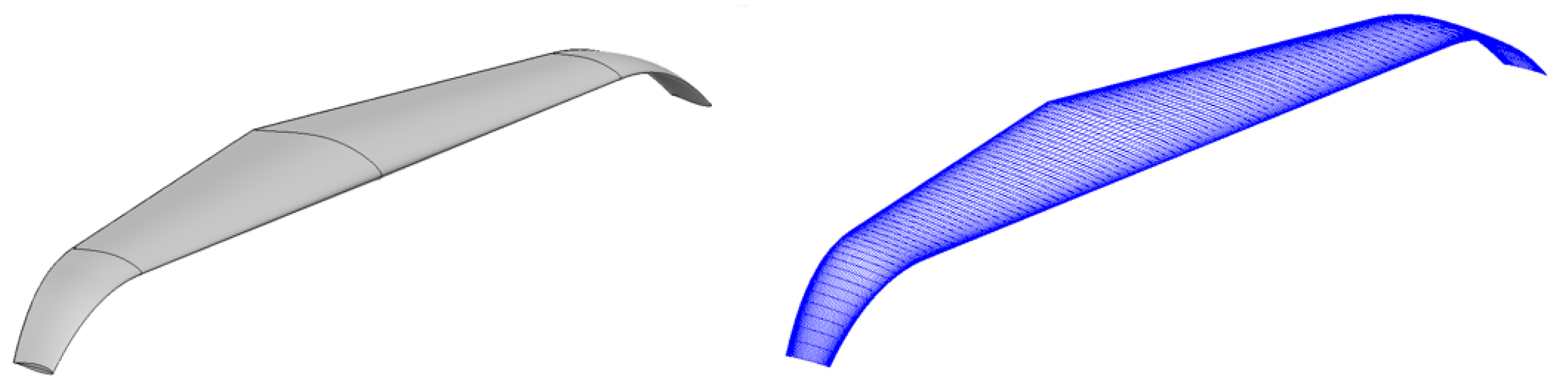
Figure 2.
Trefftz plane analysis and definition of the geometric parameters.
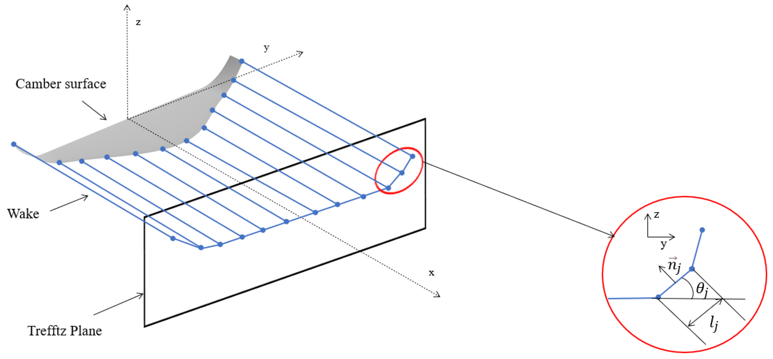
Figure 3.
Ground effect modelling using method of images.

Figure 4.
CAD model of the baseline ATR 42-600 aircraft.

Figure 5.
Influence of strength parameter: (left) and (right).
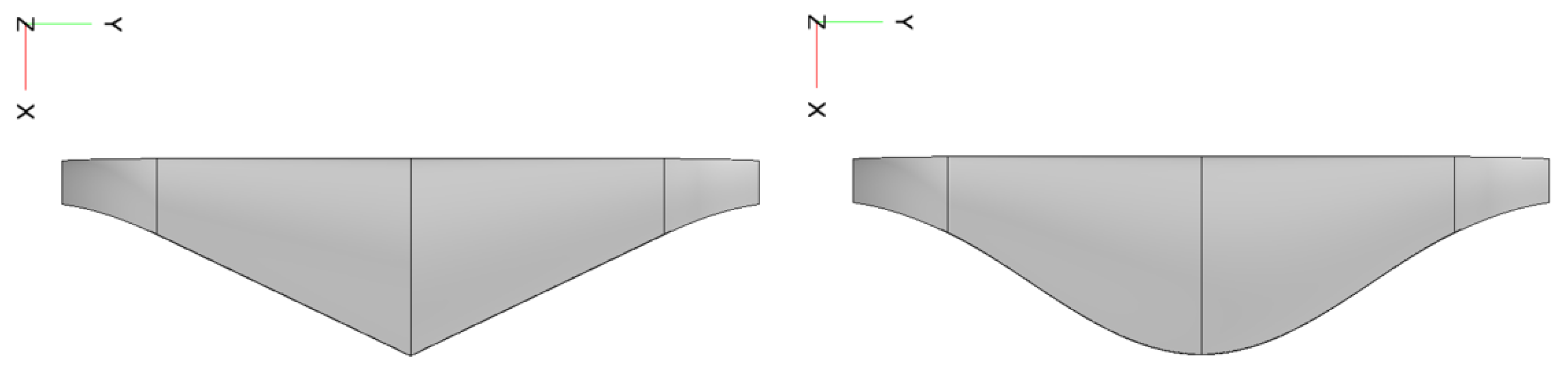
Figure 6.
Definition of wing planform design variables: (a) Case-1 (b) Case-2 (c) Case-3.
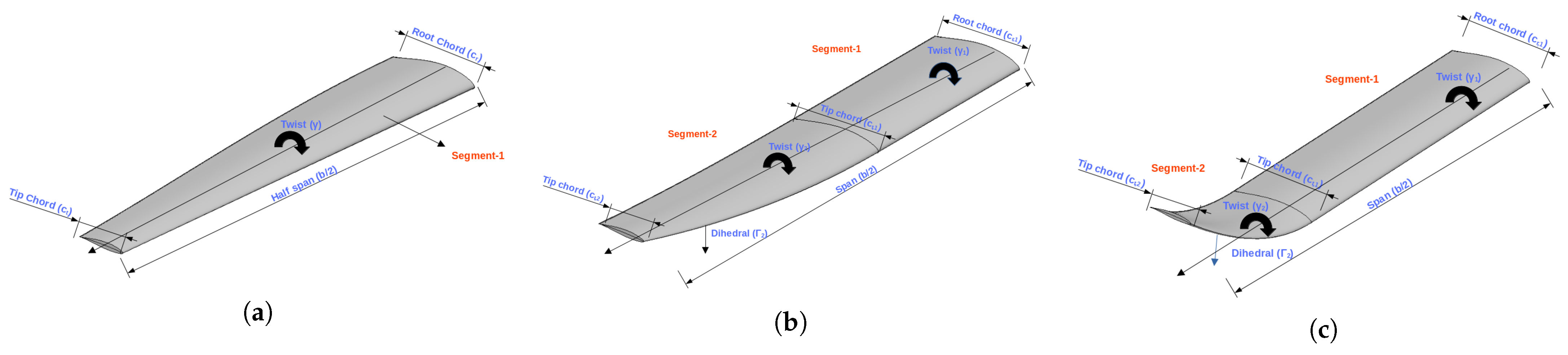
Figure 7.
Surface grid refinement results.

Figure 8.
Surface meshes on the camber surface level-L1 (top) and level-L5 (bottom) with different blending strength parameter (left), (right).
Figure 8.
Surface meshes on the camber surface level-L1 (top) and level-L5 (bottom) with different blending strength parameter (left), (right).

Figure 9.
XDSM diagram for the multi-objective wing planform optimisation work flow.

Figure 10.
Comparison of Pareto plot for wing planform optimisation (Case-1): (a) (b) (c) .
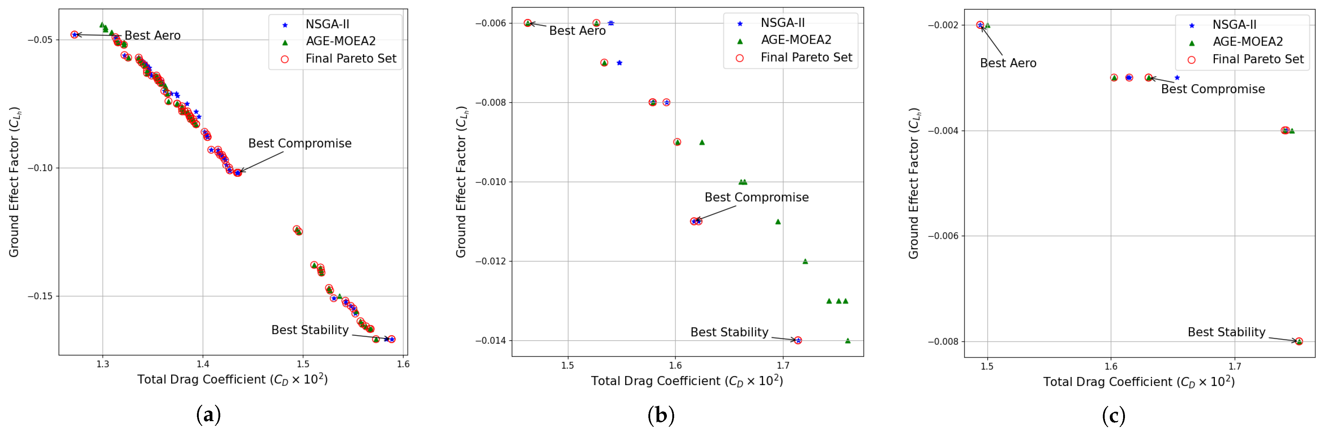
Figure 11.
Comparison of optimised wing planform shapes obtained at three different height ratios (Case-1).
Figure 11.
Comparison of optimised wing planform shapes obtained at three different height ratios (Case-1).

Figure 12.
Comparison of geometric parameters of optimised wing planform shapes (Case-1): (a) Aspect ratio vs. (b) Wing span vs. (c) Flying altitude vs. .
Figure 12.
Comparison of geometric parameters of optimised wing planform shapes (Case-1): (a) Aspect ratio vs. (b) Wing span vs. (c) Flying altitude vs. .
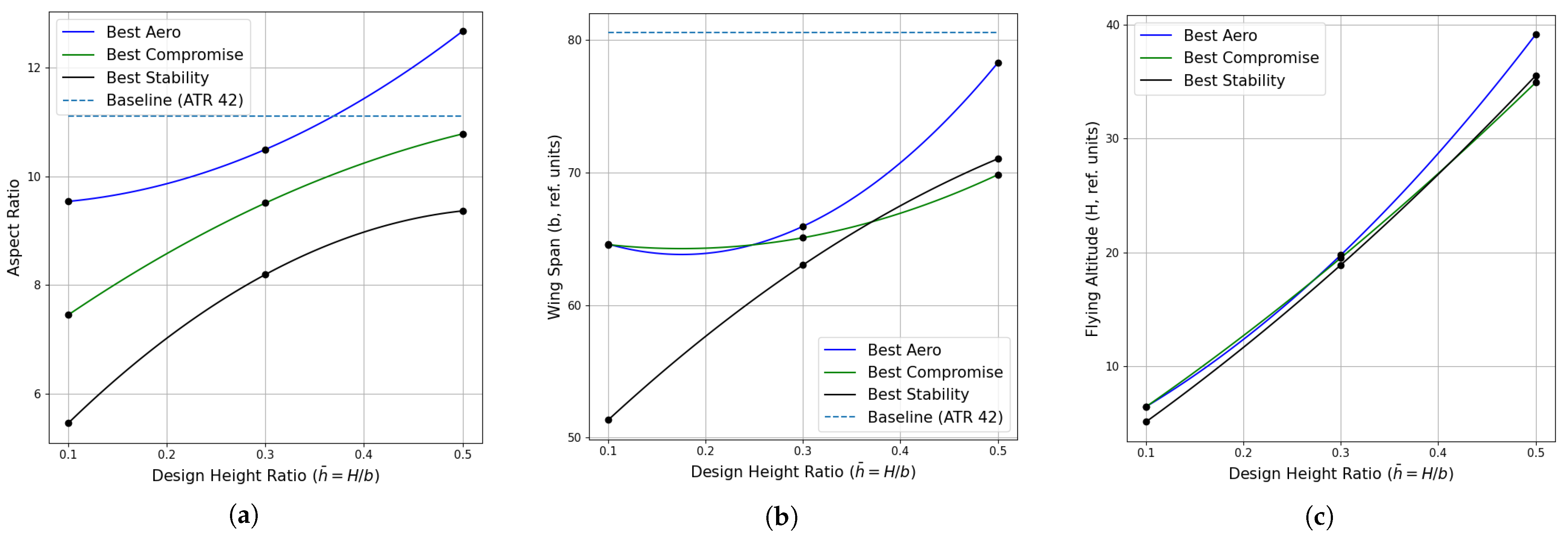
Figure 13.
Comparison of lift-to-drag ratio and ground effect factor of the optimised wing planform shapes (Case-1) obtained at each design height ratios: (a) vs. (b) vs. .
Figure 13.
Comparison of lift-to-drag ratio and ground effect factor of the optimised wing planform shapes (Case-1) obtained at each design height ratios: (a) vs. (b) vs. .

Figure 14.
Load distribution along the spanwise direction (Case-1): (a) (b) (c) .

Figure 15.
Breakdown of profile and induced drag of the best solutions obtained at (Case-1). Drag is presented relative to the baseline ATR 42 wing planform in ground effect at .
Figure 15.
Breakdown of profile and induced drag of the best solutions obtained at (Case-1). Drag is presented relative to the baseline ATR 42 wing planform in ground effect at .
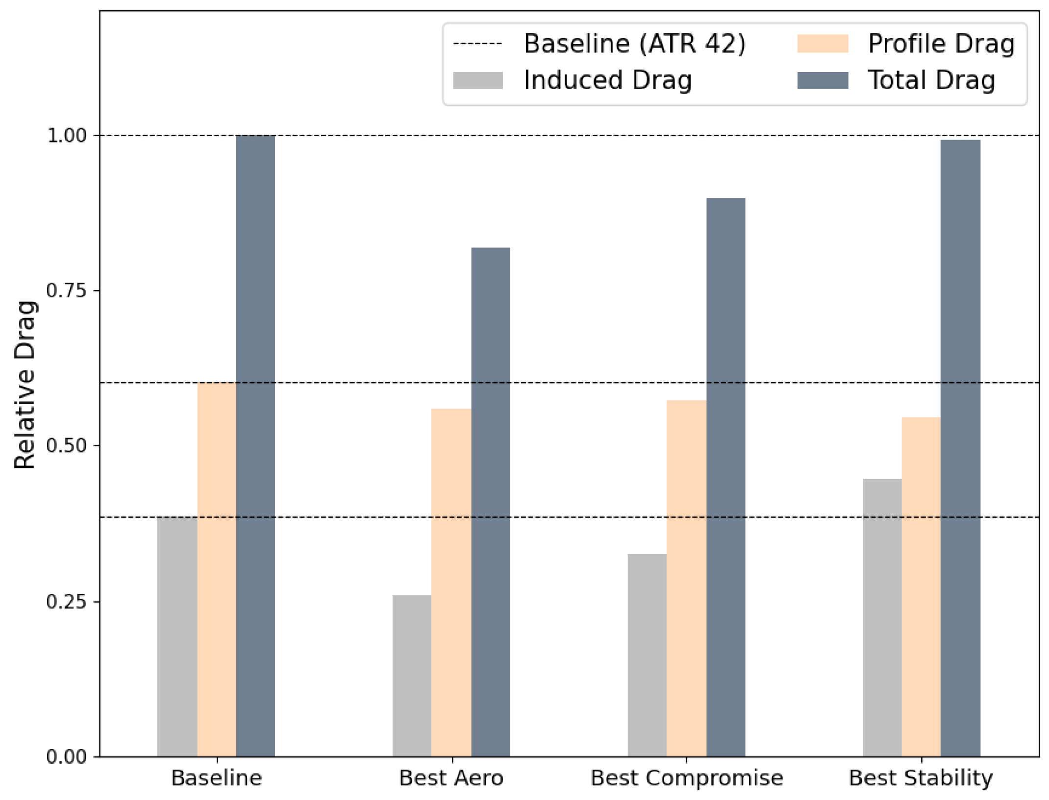
Figure 16.
Comparison of Pareto plot for nonplanar wing planform optimisation (Case-2): (a) (b) (c) .
Figure 16.
Comparison of Pareto plot for nonplanar wing planform optimisation (Case-2): (a) (b) (c) .

Figure 17.
Comparison of optimised nonplanar wing planform shapes obtained at different height ratios (Case-2).
Figure 17.
Comparison of optimised nonplanar wing planform shapes obtained at different height ratios (Case-2).

Figure 18.
Comparison of geometric parameters of optimised wing planform shapes (Case-2): (a) Dihedral angle vs. (b) Aspect ratio vs. .
Figure 18.
Comparison of geometric parameters of optimised wing planform shapes (Case-2): (a) Dihedral angle vs. (b) Aspect ratio vs. .

Figure 19.
Comparison of the normalized planform area and projected span of the optimised geometries obtained using Case-1, Case-2 and Case-3 at : (a) Normalized planform area (b) Normalized projected span.
Figure 19.
Comparison of the normalized planform area and projected span of the optimised geometries obtained using Case-1, Case-2 and Case-3 at : (a) Normalized planform area (b) Normalized projected span.
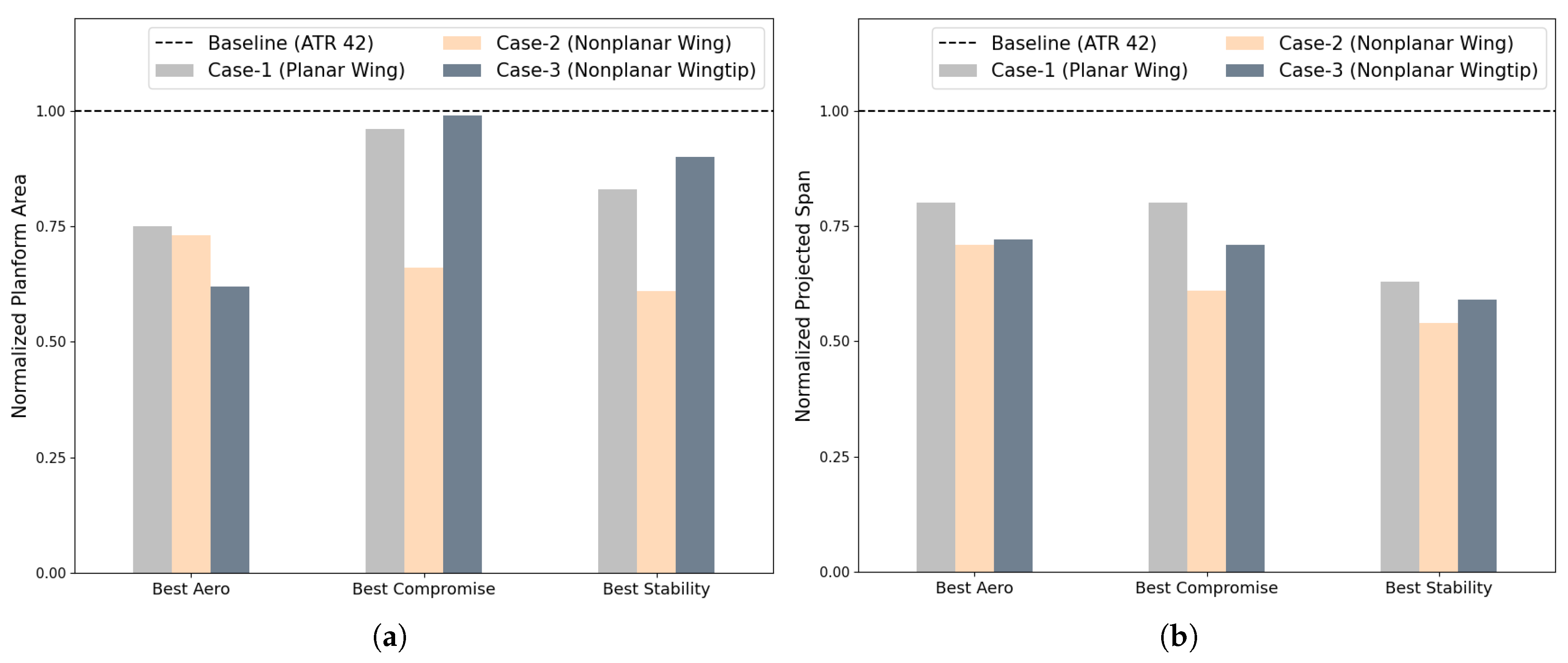
Figure 20.
Breakdown of profile drag and induced drag of the best solutions obtained at (Case-2). Drag is presented relative to the baseline ATR 42 wing planform in ground effect at .
Figure 20.
Breakdown of profile drag and induced drag of the best solutions obtained at (Case-2). Drag is presented relative to the baseline ATR 42 wing planform in ground effect at .

Figure 21.
Load distribution along the spanwise direction (Case-2): (a) (b) (c) .
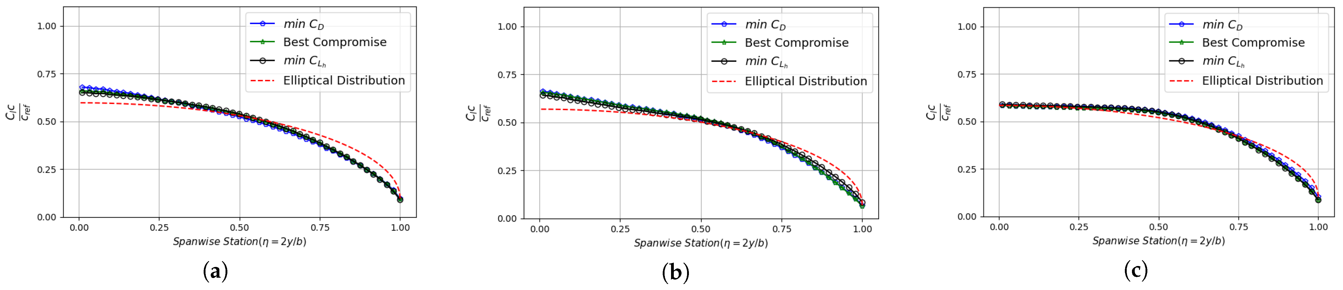
Figure 22.
Comparison of Pareto plot for wing planform optimisation (Case-3): (a) (b) (c) .
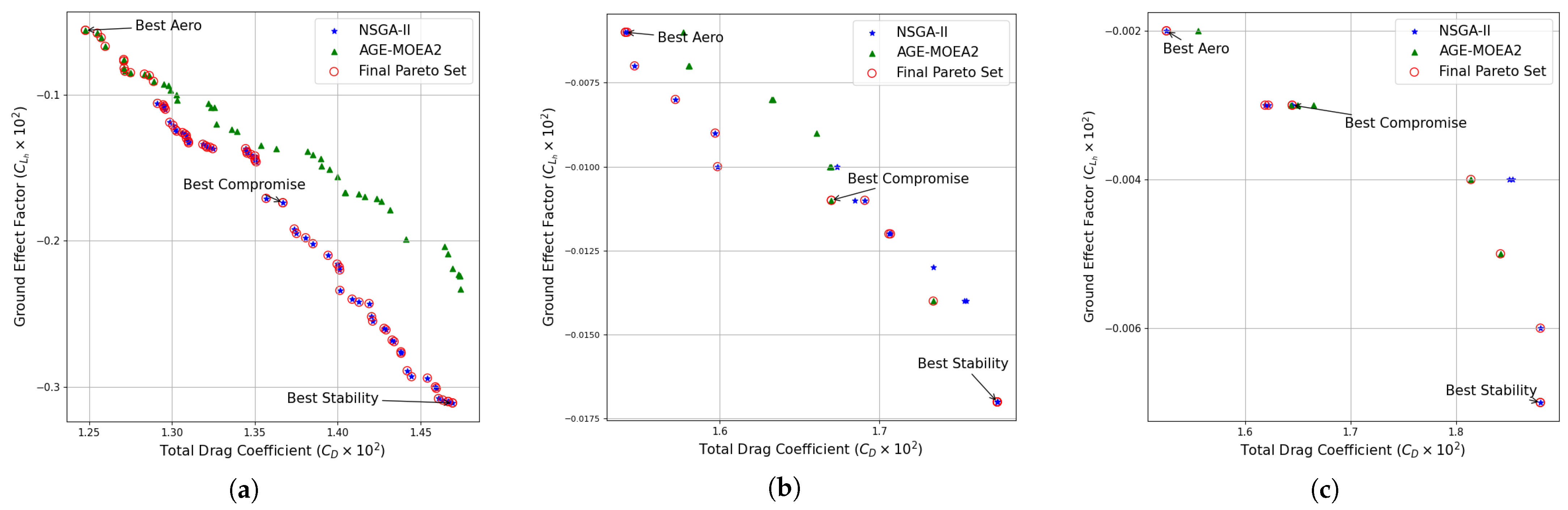
Figure 23.
Comparison of optimised nonplanar wingtip planform shapes obtained at different height ratios (Case-3).
Figure 23.
Comparison of optimised nonplanar wingtip planform shapes obtained at different height ratios (Case-3).

Figure 24.
Comparison of geometric parameters of optimised wing planform shapes (Case-3): (a) Aspect ratio vs. (b) Dihedral angle vs. (b).
Figure 24.
Comparison of geometric parameters of optimised wing planform shapes (Case-3): (a) Aspect ratio vs. (b) Dihedral angle vs. (b).
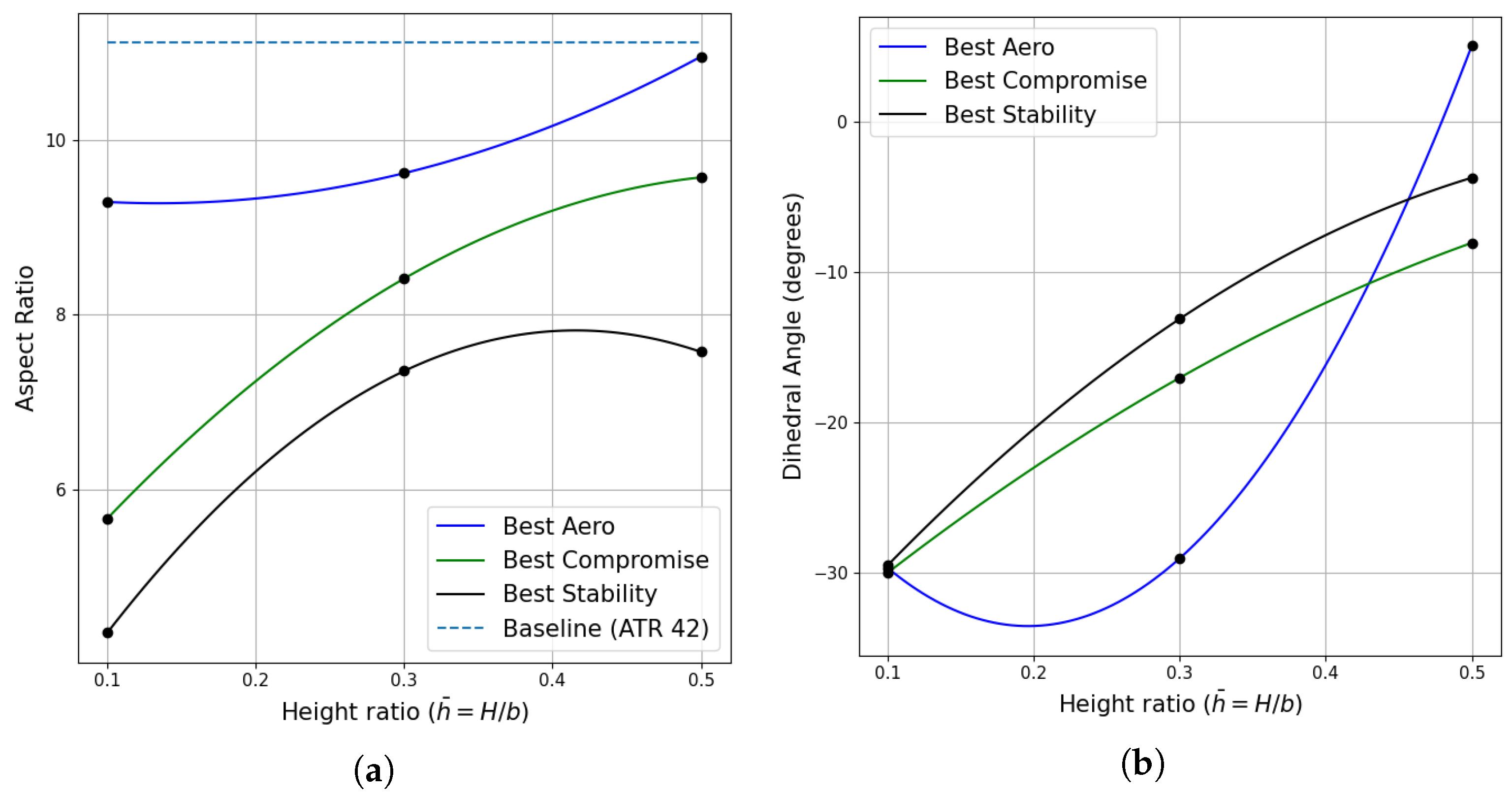
Figure 25.
Load distribution along the spanwise direction (Case-3): (a) (b) (c) .
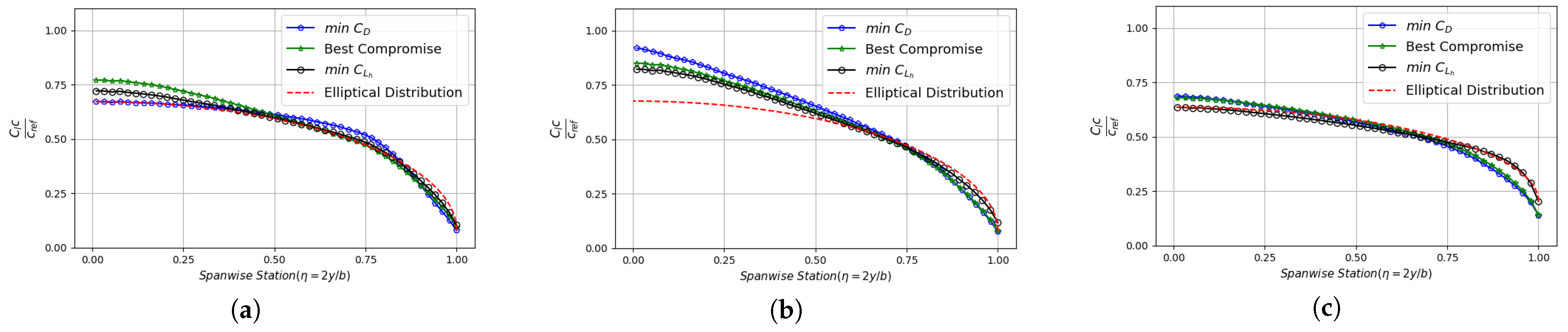
Figure 26.
Breakdown of profile drag and induced drag for best the solutions obtained at (Case-3). Drag is presented relative to the baseline ATR 42 wing planform in ground effect at .
Figure 26.
Breakdown of profile drag and induced drag for best the solutions obtained at (Case-3). Drag is presented relative to the baseline ATR 42 wing planform in ground effect at .


Table 1.
Baseline ATR 42-600 design summary.
| Design Specifications | Value |
|---|---|
| Wing Reference Area | 587 ft |
| Wing Span | 81 ft |
| Aspect Ratio | |
| Taper Ratio | |
| Root | |
| Tip | |
| Sweep | |
| Dihedral |
Table 2.
Bounds for the design variables.
| Category | Name | Lower Limit | Upper Limit | Units |
|---|---|---|---|---|
| Objective Function | min | - | ||
| min | - | |||
| Case-1: Design Variables | AOA | 5 | Degrees | |
| Twist | 5 | Degrees | ||
| Root chord | Ref. units | |||
| Tip chord | Ref. units | |||
| Blend Strength | 0 | 1 | Ref. units | |
| Span | Ref. units | |||
| Case 2: Design Variables | 5 | Degrees | ||
| 5 | Degrees | |||
| 0 | 1 | Ref. units | ||
| Ref. units | ||||
| Ref. units | ||||
| 5 | Degrees | |||
| Ref. units | ||||
| 5 | Degrees | |||
| b | Ref. units | |||
| Case 3: Other design variables same as Case 2 | −30 | 30 | Degrees | |
| 0 | 5 | Degrees |
Table 3.
Parameters used in NSGA-II and AGE-MOEA2.
| Parameters | Case | Value |
|---|---|---|
| No. of Populations | Case-1 | 60 |
| Case-2 | 90 | |
| Case-3 | 100 | |
| No. of Generations | Case-1 | 72 |
| Case-2 | 108 | |
| Case-3 | 120 | |
| Crossover Probability | 0.9 | |
| Mutattion Probability | ||
Table 4.
Case-1 optimisation results with design lift coefficient, .
| Solution | Design Height Ratio | Design Height Ratio | Design Height Ratio | ||||||
|---|---|---|---|---|---|---|---|---|---|
| min | 0.1 | −18.17 | 1.2 | 0.3 | −18.72 | 1.0 | 0.5 | −21.35 | 1.0 |
| Best Compromise | −10.28 | 2.5 | −10.14 | 1.8 | −14.19 | 1.5 | |||
| min | −0.71 | 4.1 | −4.78 | 2.3 | −7.78 | 4.0 |
Table 5.
Case-2 optimisation results with design lift coefficient, .
| Solution | Design Height Ratio | Design Height Ratio | Design Height Ratio | ||||||
|---|---|---|---|---|---|---|---|---|---|
| min | 0.1 | −19.0 | 1.9 | 0.3 | −11.0 | 1.2 | 0.5 | −21.42 | 1.0 |
| Best Compromise | −11.45 | 3.1 | −10.24 | 1.5 | −20.46 | 1.5 | |||
| min | −5.1 | 4.4 | −7.53 | 2.0 | −13.55 | 3.5 |
Table 6.
Case-3 optimisation results with design lift coefficient, .
| Solution | Design Height Ratio | Design Height Ratio | Design Height Ratio | ||||||
|---|---|---|---|---|---|---|---|---|---|
| min | 0.1 | −22.0 | 1.4 | 0.3 | −14.39 | 1.0 | 0.5 | −19.71 | 1.0 |
| Best Compromise | −14.56 | 4.34 | −7.22 | 1.8 | −13.43 | 1.5 | |||
| min | −8.16 | 7.7 | −1.46 | 2.8 | −1.05 | 3.5 |
Disclaimer/Publisher’s Note: The statements, opinions and data contained in all publications are solely those of the individual author(s) and contributor(s) and not of MDPI and/or the editor(s). MDPI and/or the editor(s) disclaim responsibility for any injury to people or property resulting from any ideas, methods, instructions or products referred to in the content. |
© 2023 by the authors. Licensee MDPI, Basel, Switzerland. This article is an open access article distributed under the terms and conditions of the Creative Commons Attribution (CC BY) license (https://creativecommons.org/licenses/by/4.0/).
Share and Cite
MDPI and ACS Style
Jesudasan, R.; Hanifi, A.; Mariani, R. Investigating Planar and Nonplanar Wing Planform Optimisation for Ground Effect Aircraft. Aerospace 2023, 10, 969. https://doi.org/10.3390/aerospace10110969
AMA Style
Jesudasan R, Hanifi A, Mariani R. Investigating Planar and Nonplanar Wing Planform Optimisation for Ground Effect Aircraft. Aerospace. 2023; 10(11):969. https://doi.org/10.3390/aerospace10110969
Chicago/Turabian StyleJesudasan, Rejish, Ardeshir Hanifi, and Raffaello Mariani. 2023. "Investigating Planar and Nonplanar Wing Planform Optimisation for Ground Effect Aircraft" Aerospace 10, no. 11: 969. https://doi.org/10.3390/aerospace10110969
Note that from the first issue of 2016, this journal uses article numbers instead of page numbers. See further details here.