
Modeling and Disturbance Analysis of Spinning Satellites with Inflatable Protective Structures

Faculty of Electronic and Information Engineering, Xi’an Jiaotong University, Xi’an 710049, China
*
Author to whom correspondence should be addressed.
Aerospace 2023, 10(11), 971; https://doi.org/10.3390/aerospace10110971
Submission received: 9 October 2023
/
Revised: 2 November 2023
/
Accepted: 15 November 2023
/
Published: 18 November 2023
Abstract
:The escalating proliferation of space debris poses an increasing risk to spinning satellites, elevating the probability of hazardous collisions that can result in severe damage or total loss of functionality. To address this concern, a pioneering inflatable protective structure is employed to ensure the optimal functionality of spinning satellites. Additionally, a multi-body dynamic modeling method based on spring hinge unfolding/spring expansion is proposed to tackle the complex dynamics of spinning satellites with inflatable protective structures during flight. This method enables analysis of the motion parameters of spinning satellites. First, the structural composition of a spinning satellite with inflatable protective structures is introduced and its flight process is analyzed. Then, an articulated spring hinge unfolding model or a spring expansion model using the Newton–Euler method is established to describe the unfolding or expansion of the spinning satellite with inflatable protective structures during flight. Finally, the effects on the motion parameters of a spinning satellite are analyzed through simulation under various working conditions.
1. Introduction
As a class of satellites with simple structures that are extremely reliable, spinning satellites maintain attitude stability in space through rotation, allowing them to complete specific tasks at a lower cost [1,2,3,4]. With the rapid advancement of human space exploration, there has been a significant increase in the accumulation of space debris. The surge in space debris poses a substantial threat to spinning satellites, as they may collide with space debris during their operation, leading to severe damage or even mission failure [5,6,7,8]. Consequently, ensuring the smooth operation and extended lifespan of spinning satellites and effectively tackling the threat posed by space debris has emerged as a prominent research focus in the aerospace sector.
Inflatable structures have been in development for various space applications since the 1950s [9,10,11,12,13]. In the late 1950s, the limited history of inflatable protective structures began with work conducted by NASA on the Echo balloon program [9]. In 1960, the Erectable Torus Manned Space Laboratory concept was proposed by Goodyear Aircraft Corporation [10]. In the late 1960s, L’Garde Incorporated tested inflatable exoatmospheric objects (IEOs) as decoys for the Mark 12 nuclear warhead reentry vehicle [11]. Freefall Aerospace along with the University of Arizona developed inflatable spherical antenna systems for small satellites [12]. Jet Propulsion Laboratory developed an inflatable perimeter-truss structure supporting a mesh/net parabolic reflector antenna [13]. Notably, inflatable structures offer a valuable means of providing an additional layer of protection. Consequently, the utilization of inflatable structures is an effective means of mitigating the threat posed by space debris.
The inflation of novel IPSs during flight may introduce additional disturbances to spinning satellites, leading to deviations in their motion parameters. To analyze the disturbances in the motion parameters of spinning satellites, it is imperative to develop dynamic models of spinning satellites with IPSs. The modeling problem of spinning satellites with IPSs involves a complex coupling between rigid and flexible bodies. The IPSs, as flexible bodies, interact with spinning satellites, which are treated as rigid bodies. This dynamic interaction gives rise to challenging a rigid–flexible coupling. The predominant modeling approaches used to address this issue include the finite element method [14,15,16], the multi-body dynamic method [17,18,19], as well as the mixed method, among others [20,21,22]. For instance, Ref. [14] proposed a rigid–flexible coupling dynamic model to investigate a gearbox system-level transmission error, incorporating a meshing pair, flexible shaft, and bearing using lumped mass, beam, and spring elements, respectively. Housing flexibility was considered through model condensation, and validation was performed using modal and transmission error tests. In [18], a 14-degree-of-freedom flexible multi-body dynamic model for a semi-submersible floating offshore wind turbine was developed and verified against fast simulation results from the US National Renewable Energy Laboratory for free decay and various wind–wave load cases. Ref. [20] presented a novel analytical method that integrates multi-body dynamics and finite element analysis to simulate lateral and torsional vibrations in a single rotor system, with a focus on studying the effects of these vibrations on the bearings and the mass center due to increased operating speeds and eccentricity in the industry. To expedite the simulation process, the multi-body dynamic method is employed to construct dynamic models of spinning satellites with IPSs.
In the realm of dynamic modeling for multi-body systems, customary approaches draw upon fundamental principles of dynamics, including the venerable Newton–Euler equations [23,24,25], Kane equations [26,27,28], and Lagrange equations of the second kind [29,30,31]. For instance, to address the challenges posed by geometric non-linearity arising from significant deformations and aeroelastic behavior under severe wind conditions, Ref. [23] employed the rigid multi-body dynamic approach to develop blade analysis using a multi-body model, simulation analyses of the geometric non-linearity under static loading, and the aeroelastic response under extreme operating gust conditions. In [26], the author proposed a novel prototype of a planetary rover named ‘Archimedes’ and derived a multi-body dynamic model based on Kane’s method to implement a lumped parameter model with a rotational joint with nonlinear torque. The analytical model was validated by comparing it with simulations conducted using MSC Adams 2020 software. By using the second type of Lagrange equations, Ref. [29] formulated a rigorous mathematical model to describe the behavior of a centrifugal pendulum absorber and derived an analytical solution by employing the multiple scales method. This was then compared with the numerical simulation results obtained using all nonlinear equations of motion and the analytical solution. The integration of the Newton–Euler equation into the multi-body dynamics method presents a distinct advantage due to its inherent clarity in conveying physical significance. As a consequence, this fusion facilitates the establishment of comprehensive dynamic models for spinning satellites with IPSs.
In summary, this paper focuses on spinning satellites, introduces an innovative IPS, and presents a multi-body dynamic modeling approach based on spring hinge unfolding/spring expansion. The major contributions are in the following aspects:
- (1)
- A novel IPS is implemented to guarantee the smooth operation of spinning satellites;
- (2)
- The dynamic model of the spinning satellite with IPSs in the inflatable stage is decoupled into two separate models: the spring hinge unfolding model and the spring expansion model;
- (3)
- The multi-body dynamics method based on the Newton–Euler equations is utilized to develop both the spring hinge unfolding model and the spring expansion model;
- (4)
- Various operating conditions are taken into consideration to thoroughly analyze the effects on the spinning satellite during the unfolding or expansion of IPSs.
In addition to the above discussion and description, this paper is structured as follows: Section 2 introduces the structure and flight process of the spinning satellite with IPSs. Section 3 presents the establishment of the spring hinge unfolding model/spring expansion model. The simulation results are thoroughly discussed in Section 4. Finally, in Section 5, some conclusions drawn from this paper are summarized.
2. Description of the Spinning Satellite with IPSs
Figure 1 presents the structural composition of the spinning satellite with IPSs. It comprises a central rigid spinning satellite, followed by three evenly distributed rigid connecting shells, three equally spaced flexible IPSs, and three uniformly positioned rigid fixed covers, progressing from the innermost to the outermost layer.
During the operational course of the flight, the spinning satellite with IPSs undergoes four sequential stages: free flight, fixed covers separation, IPS inflation, and free flight. Before entering the atmosphere, during the free flight stage, the spinning satellite with IPSs is in a compressed state: the flexible IPSs are subjected to vacuum pumping (with some residual gas remaining) and subsequently deployed onto the outer surface of connecting shells. The outer surface is then secured with fixed covers, as depicted in Figure 2a. As it enters the atmosphere and reaches the fixed cover separation stage, the spinning satellite with IPSs smoothly transitions into the separation state: structures between each fixed cover and the spinning satellite are unlocked at a specific time, resulting in the complete detachment of all fixed covers from the spinning satellite, as shown in Figure 2b. After the fixed covers, the spinning satellite with IPSs enters the IPS inflatable stage and remains in the inflatable state: the flexible IPSs progressively inflate into spherical shapes at a specific time due to the influence of the remaining gas, as illustrated in Figure 2c. Once the IPSs have fully inflated, the spinning satellite with IPSs attains a stable state during the free flight stage: the spinning satellite with IPSs assumes a spherical configuration while flying in outer space, as demonstrated in Figure 2d.
Remark 1. In the realm of practical engineering, simultaneous separation of all fixed covers is unfeasible. Consequently, it is postulated that the fixed covers are sequentially separated at predetermined intervals. A similar principle applies to the inflation of the IPSs. In addition, when the spinning satellite with IPSs is in a compressed state, the flexible IPSs are vacuumed (with some residual gas remaining), and then the structure is folded in the pattern shown in Figure 3.
3. Dynamic Modeling of the Spinning Satellite with IPSs
Given that the deformation of the spinning satellite with IPSs is negligible, it can be simplified as a single rigid body. Additionally, the separation of the fixed cover is assumed to occur instantaneously, resulting in a short duration. Therefore, the focus of the dynamic modeling lies in capturing the behavior of the spinning satellite with IPSs in the inflatable stage. To streamline the modeling process and facilitate efficient computations, the dynamic model of the spinning satellite with IPSs is established with the multi-body dynamics method [32]. Considering the state of the spinning satellite with IPSs at the onset of the inflatable stage, this stage is simplified as the unfolding processes under spring hinge connections and the expansion process under spring connections. Consequently, this section primarily focuses on establishing the spring hinge unfolding model and the spring expansion model.
3.1. Spring Hinge Unfolding Model
Considering there is only one degree of freedom, specifically the relative rotation at the hinge, between three IPSs and the spinning satellite, all spring hinges are simplified as line segments in three-dimensional space. The spring hinge unfolding model, depicted in Figure 4, is established accordingly.
According to the Newton–Euler equation [33], the dynamics equation of the spinning satellite and the kth IPS relative to the reference frame can be expressed as
where is the force at the kth spring hinge, and and are the torques at the kth spring hinge in Ou0 and Ouk.
By eliminating Fudk, and in (1), we can obtain
where is the coordinate conversion matrix that transforms Ouk into Ou0. According to the geometric constraint relationship between the kth IPS and the spinning satellite, we have
where is the coordinate conversion matrix that transforms Ou0 into Ou, is the coordinate conversion matrix that transforms Ouk into Ou, is the angular displacement at the kth spring hinge, and are the installation positions on the kth line segment in Ou0 and Ouk, , and are the unit directions on the kth line segment in Ou0 and Ouk. is the quaternion that describes Ouk with respect to Ou0, which is expressed as . Taking the derivative of (3), we obtain
where is the angular velocity that describes Ouk with respect to Ou0, which is expressed as . Based on (2) and (4), we have
Taking the derivative of (5), we obtain
By substituting (6) into (2), we have
The kth spring hinge can be modeled as a spring–damping system, which can be expressed as follows:
where K is the stiffness coefficient and is the damping coefficient.
According to (1), (7), and (8), we can have
where
Through the dynamics model (9), the effect of the unfolding process under the spring hinge connection can be analyzed.
3.2. Spring Expansion Model
To simplify the dynamic analysis, a spring expansion model, as illustrated in Figure 5, is established.
According to the Newton–Euler equation, the dynamic equation of the spinning satellite and the kth IPS relative to the reference frame can be expressed as
where Fedk is the force at the kth spring, and are the torques at the kth spring hinge in Oe0 and Oek.
The kth spring can be modeled as a spring–damping system, and its mathematical expression is given by the following equation:
where are stiffness coefficients, and are damping coefficients. Fedk,k is the force at the kth spring in Oek. is the installation position of the kth spring in Oe0. is the coordinate conversion matrix that transforms Oek into Oe, and is the coordinate conversion matrix that transforms Oek into Oe0. is the quaternion that describes Oek with respect to Oe0. , , and can be expressed as
Through the dynamics model (11), the disturbance effect of the expansion process under the spring connection can be analyzed.
4. Simulation Results and Analysis
In this section, we provide a thorough analysis of the disturbances caused by the unfolding or expansion of the motion parameters of the spinning satellite under various working conditions. The parameter values of the spinning satellite with IPSs are shown in Table 1.
4.1. IPS Unfolding Analysis
To comprehensively analyze the effect caused by IPSs on the spinning satellite, two distinct working conditions with unfolding intervals of 0.01 s and 0.4 s are carefully chosen for the simulation analysis. Subsequently, two types of curves are plotted to illustrate the findings and observations derived from the analysis.
- The deviation motion curve of the spinning satellite between IPSs in the orbital coordinate system and free flight in the same orbital coordinate system is
- The disturbance force and torque curve of the spinning satellite in the spinning satellite coordinate system are
4.1.1. Unfolding Interval of 0.01 s
Figure 6 illustrates the deviation motion curves of the spinning satellite during IPSs using an unfolding interval of 0.01 s in the orbital coordinate system. From (a) to (d), it is evident that, given the simulation parameters, the duration of IPS unfolding amounts to approximately 0.59 s. Throughout the unfolding process, the spinning satellite undergoes deviations with magnitudes on the order of 10−2 m in displacement, 10−2 m per second in velocity, 100 degrees in angular displacement, and 10−1 revolutions per second in angular velocity.
Figure 7 shows the disturbance force/torque curves in the spinning satellite coordinate system using an unfolding interval of 0.01 s. (a) and (b) reveal that the disturbance forces exerted on the spinning satellite are approximately 101 Newtons in magnitude, while the disturbance torques reach an approximate magnitude of 101 Newton meters. The resulting impact of these disturbance forces and torques on the satellite’s velocities and angular velocities induces changes in its momenta and angular momenta, respectively, which manifest as impulses and angular impulses. Through rigorous calculations, the impulses caused by the disturbance are approximately 10−1 Newtons per second in magnitude, and the angular impulses amount to an approximate magnitude of 10−1 Newton meters per second.
4.1.2. Unfolding Interval of 0.4 s
Figure 8 depicts the deviation motion curves of the spinning satellite during IPS unfolding using the unfolding interval of 0.4 s in the orbital coordinate system. Based on (a) to (d), it can be observed that, for the prescribed simulation parameters, the duration of IPS unfolding amounts to approximately 1.2 s. During the unfolding process, the displacement deviations of the spinning satellite are on the order of 10−2 m, the velocity deviations are on the order of 10−2 m per second, the angular displacement deviations are on the order of 100 degrees, and the angular velocity deviations are on the order of 10−1 revolutions per second.
Figure 9 shows the disturbance force/torque curves in the spinning satellite coordinate system using the unfolding interval of 0.4 s. Both (a) and (b) indicate that the disturbance forces applied to the spinning satellite are approximately a magnitude of 101 Newtons, while the disturbance torques reach a magnitude of 101 Newton meters.
4.2. IPS Expansion Analysis
To comprehensively analyze the effect of IPS expansion on the spinning satellite, two distinct working conditions are judiciously chosen, characterized by unfolding intervals of 0.01 s and 0.08 s, to conduct the simulation analysis. Subsequently, two types of curves are meticulously constructed to visually represent the significant findings and pertinent observations derived from the conducted analysis.
- The deviation motion curve of the spinning satellite between IPS expansion in the orbital coordinate system and free flight in the same orbital coordinate system is
- The disturbance force and torque curve of the spinning satellite in the spinning satellite coordinate system are
4.2.1. Expansion Interval of 0.01 s
Figure 10 illustrates the deviation motion curves of the spinning satellite during IPS expansion using the expansion interval of 0.01 s in the orbital coordinate system. Based on the presented (a)–(d), it is evident that, given the simulation parameters, the temporal span of IPS expansion amounts to approximately 0.14 s. During the expansion process, the spinning satellite’s velocities undergo deviations on the order of 10−1 m per second. Once the IPSs reach their maximum capacity and undergo sudden tightening, the spinning satellite’s velocities experience significant deviations on the order of 100 m per second. Throughout the procedure, the spinning satellite exhibits displacement deviations on the order of 10−2 m, while its angular velocities experience deviations of approximately 10−3 rotations per second. Additionally, the angular displacements encounter deviations on the order of 10−2 degrees.
Figure 11 shows the disturbance force/torque curves in the spinning satellite coordinate system using the expansion interval of 0.01 s. During the expansion process, the spinning satellite is anticipated to encounter disturbance forces approximately on the order of 102 newtons. Once the IPSs are fully expanded, the disturbance forces are expected to escalate to the order of 105 newtons, leading to a sudden tightening of the flexible body. Moreover, the expansion procedure induces the disturbance torques on the order of 101 Newton meters.
4.2.2. Expansion Interval of 0.08 s
Figure 12 illustrates the deviation motion curves of the spinning satellite during IPS expansion using the expansion interval of 0.08 s in the orbital coordinate system. Based on (a)–(d), it is evident that, within the specified simulation parameters, the IPS expansion duration is approximately 0.22 s. During the expansion process, the spinning satellite undergoes velocity deviations on the order of 10−1 m per second. Upon reaching its limit and experiencing instantaneous tension, the velocity deviations increase to the order of 100 m per second. Throughout the entire expansion process, the displacements result in deviations on the order of 10−2 m. Additionally, the spinning satellite’s angular velocities experience deviations on the order of 10−3 rotations per second, while the angular displacements encounter deviations on the order of 10−2 degrees.
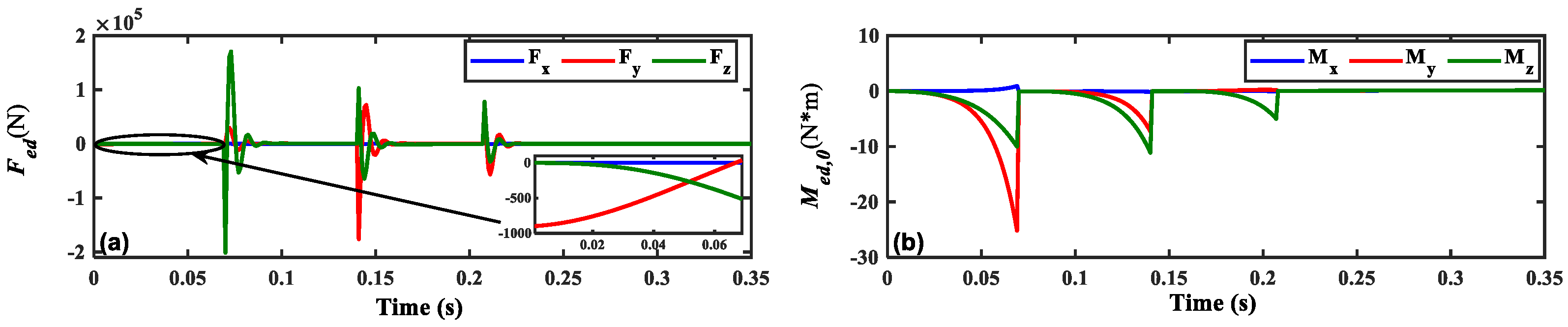
Figure 13 shows the disturbance force/torque curves in the satellite coordinate system using the expansion interval of 0.08 s. During the expansion process, the spinning satellite experiences disturbance forces of approximately an order of 102 Newtons. When the IPSs reach their maximum expansion, the disturbance forces reach an order of approximately 105 Newtons, causing the IPSs to tighten instantaneously. Additionally, the expansion process generates disturbance torques on the order of approximately 101 Newton meters.
4.3. Dynamic Model Verification
To verify the correctness of the dynamic model, a finite element model based on ABAQUS is adopted. First, the three-dimensional model of the spinning satellite with IPSs in the inflatable state is established in SolidWorks 2022 software. Then, it is imported into ABAQUS 2022 software to calculate and analyze the IPS process.
Table 2 summarizes the RMS comparison of the calculation results of the finite element model and the proposed dynamic model. It is observed that compared with the finite element model, the RMS values with the proposed dynamic model have changed within a small range of no more than 4.1084%, which illustrates the correctness of the proposed dynamic model.
5. Conclusions
This paper proposes a multi-body dynamic modeling approach based on an unfolding model and spring expansion model for a spinning satellite with IPSs. First, a pioneering IPS is employed to address the hazard posed by space debris to spinning satellites. Then, the dynamic model of the spinning satellite with IPSs in the inflatable stage is divided into the spring hinge unfolding model and the spring expansion model; both the spring hinge unfolding model and the spring expansion model are established using the multi-body dynamic method based on the Newton–Euler equations. Finally, considering different time intervals, the effect on the motion parameters of the spinning satellite is analyzed comprehensively during the unfolding or expansion of IPSs.
Author Contributions
The contributions of the authors are as follows: conceptualization, Y.C. (Yuanli Cai); methodology, Y.D.; software, Y.S.; validation, Y.S.; formal analysis, Y.S.; investigation, Y.C.(Yu Chen), S.H. and X.L.; resources, Y.S.; data curation, Y.S.; writing—original draft preparation, Y.S.; writing—review and editing, Y.D., H.J. and Y.C. (Yuanli Cai); visualization, Y.S.; supervision, Y.C. (Yuanli Cai); project administration, Y.C. (Yuanli Cai); funding acquisition, Y.C. All authors have read and agreed to the published version of the manuscript.
Funding
This research received no external funding.
Data Availability Statement
All data used during the study appear in the submitted article.
Conflicts of Interest
The authors declare no conflict of interest.
Nomenclature
| u | spring hinge unfolding | e | spring expansion |
| Ou | the composite center-of-mass orbital coordinate system (the reference frame) | Oe | the composite center-of-mass orbital coordinate system (the reference frame) |
| Ou0 | the spinning satellite coordinate system | Oe0 | the spinning satellite coordinate system |
| mu0 | the mass of the spinning satellite | me0 | the mass of the spinning satellite |
| Ju0 | the moment of inertia of the satellite | Je0 | the moment of inertia of the satellite |
| ru0 | the displacement of the spinning satellite | re0 | the displacement of the spinning satellite |
| qu0 | the quaternion of the spinning satellite | qe0 | the quaternion of the spinning satellite |
| vu0 | the velocity of the spinning satellite | ve0 | the velocity of the spinning satellite |
| wu0,0 | the angular velocity of the satellite in Ou0 | we0,0 | the angular velocity of the satellite in Oe0 |
| k | number of IPSs | k | number of IPSs |
| Ouk | the kth IPS coordinate system | Oek | the kth IPS coordinate system |
| muk | the mass of the kth IPS | mek | the mass of the kth IPS |
| Juk | the moment of inertia of the kth IPS | Jek | the moment of inertia of the kth IPS |
| ruk | the displacement of the kth IPS | rek | the displacement of the kth IPS |
| quk | the quaternion of the kth IPS | qek | the quaternion of the kth IPS |
| vuk | the velocity of the kth IPS | vek | the velocity of the kth IPS |
| wuk,k | the angular velocity of the kth IPS in Ouk | wek,k | the angular velocity of the kth IPS in Oek |
References
- Janssens, F.L.; van der Ha, J.C. On the stability of spinning satellites. Acta Astronaut. 2011, 68, 778–789. [Google Scholar] [CrossRef]
- Ergin, E.I.; Wheeler, P.C. Magnetic attitude control of a spinning satellite. J. Spacecr. Rocket. 1965, 2, 846–850. [Google Scholar] [CrossRef]
- Kane, T.R.; Barba, P.M. Effects of energy dissipation on a spinning satellite. AIAA J. 1966, 4, 1391–1394. [Google Scholar] [CrossRef]
- Janssens, F.L.; van der Ha, J.C. Stability of spinning satellite under axial thrust and internal mass motion. Acta Astronaut. 2014, 94, 502–514. [Google Scholar] [CrossRef]
- Greenbaum, D. Space debris puts exploration at risk. Science 2020, 370, 922. [Google Scholar] [CrossRef]
- Anttonen, A.; Kiviranta, M.; Höyhtyä, M. Space debris detection over intersatellite communication signals. Acta Astronaut. 2021, 187, 156–166. [Google Scholar] [CrossRef]
- Botta, E.M.; Sharf, I.; Misra, A.K. Simulation of tether-nets for capture of space debris and small asteroids. Acta Astronaut. 2019, 155, 448–461. [Google Scholar] [CrossRef]
- Svotina, V.V.; Cherkasova, M.V. Space debris removal–Review of technologies and techniques. Flexible or virtual connection between space debris and service spacecraft. Acta Astronaut. 2022, 204, 840–853. [Google Scholar] [CrossRef]
- Litteken, D.A. Inflatable technology: Using flexible materials to make large structures. Electroact. Polym. Actuators Devices 2019, 10966, 1096603. [Google Scholar]
- Harris, J. Advanced material and assembly methods for inflatable structures. In Proceedings of the 4th Aerodynamic Deceleration Systems Conference, Palm Springs, CA, USA, 21–23 May 1973. [Google Scholar]
- Cobb, R.G.; Black, J.T.; Swenson, E.D. Design and flight qualification of the rigidizable inflatable get-away-special experiment. J. Spacecr. Rocket. 2010, 47, 659–669. [Google Scholar] [CrossRef]
- Chandra, A.; Tonazzi, J.C.L.; Stetson, D.; Pat, T.; Walker, C.K. Inflatable membrane antennas for small satellites. In Proceedings of the 2020 IEEE Aerospace Conference, Big Sky, MT, USA, 7–14 March 2020. [Google Scholar]
- Freeland, R.E.; Helms, R.G.; Willis, P.B.; Mikulas, M.M.; Stuckey, W.; Steckel, G.; Watson, J. Inflatable space structures technology development for large radar antennas. In Proceedings of the 55th International Astronautical Congress, Vancouver, BC, Canada, 4–8 October 2004. [Google Scholar]
- Duan, T.; Wei, J.; Zhang, A.; Xu, Z.; Lim, T.C. Transmission error investigation of gearbox using rigid-flexible coupling dynamic model: Theoretical analysis and experiments. Mech. Mach. Theory 2021, 157, 104213. [Google Scholar] [CrossRef]
- Zhang, J.; Zhu, T.; Yang, B.; Wang, X.; Xiao, S.; Yang, G.; Liu, Y.; Che, Q. A rigid–flexible coupling finite element model of coupler for analyzing train instability behavior during collision. Railw. Eng. Sci. 2023, 4, 325–339. [Google Scholar] [CrossRef]
- Pagaimo, J.; Millan, P.; Ambrósio, J. Flexible multibody formulation using finite elements with 3 DoF per node with application in railway dynamics. Multibody Syst. Dyn. 2023, 30, 83–112. [Google Scholar] [CrossRef]
- Otsuka, K.; Wang, Y.; Palacios, R.; Makihara, K. Strain-based geometrically nonlinear beam formulation for rigid–flexible multibody dynamic analysis. AIAA J. 2022, 60, 4954–4968. [Google Scholar] [CrossRef]
- Luo, Y.; Qian, F.; Sun, H.; Wang, X.; Chen, A.; Zuo, L. Rigid-flexible coupling multi-body dynamics modeling of a semi-submersible floating offshore wind turbine. Ocean Eng. 2023, 281, 114648. [Google Scholar] [CrossRef]
- Htun, T.Z.; Suzuki, H.; García-Vallejo, D. On the theory and application of absolute coordinates-based multibody modelling of the rigid–flexible coupled dynamics of a deep-sea ROV-TMS (tether management system) integrated model. Ocean Eng. 2022, 258, 111748. [Google Scholar] [CrossRef]
- Eisa, A.I.; Shusen, L.; Helal, W.M. Study on the lateral and torsional vibration of single rotor-system using an integrated multi-body dynamics and finite element analysis. Adv. Mech. Eng. 2020, 12, 168. [Google Scholar] [CrossRef]
- Kashyzadeh, K.R.; Farrahi, G.H. Improvement of HCF life of automotive safety components considering a novel design of wheel alignment based on a Hybrid multibody dynamic, finite element, and data mining techniques. Eng. Fail Anal. 2023, 143, 106932. [Google Scholar] [CrossRef]
- Zhang, J.; Chen, Z.; Wang, L.; Li, D.; Jin, Z. A patient-specific wear prediction framework for an artificial knee joint with coupled musculoskeletal multibody-dynamics and finite element analysis. Tribol. Int. 2017, 109, 382–389. [Google Scholar] [CrossRef]
- Xu, J.; Zhang, L.; Li, X.; Li, S.; Yang, K. A study of dynamic response of a wind turbine blade based on the multi-body dynamics method. Renew. Energy 2020, 155, 358–368. [Google Scholar] [CrossRef]
- Wu, X.; Cui, H.; Chen, W.; Xie, Y.; Zhao, H.; Bai, W. Integral dynamics modelling of chain-like space robot based on n-order dual number. Acta Astronaut. 2020, 177, 552–560. [Google Scholar]
- Gießler, M.; Waltersberger, B. Robust inverse dynamics by evaluating Newton–Euler equations with respect to a moving reference and measuring angular acceleration. Auton Robot. 2023, 47, 465–481. [Google Scholar]
- Caruso, M.; Bregant, L.; Gallina, P.; Seriani, S. Design and multi-body dynamic analysis of the Archimede space exploration rover. Acta Astronaut. 2022, 194, 229–241. [Google Scholar]
- Sarkar, S.; Fitzgerald, B. Use of kane’s method for multi-body dynamic modelling and control of spar-type floating offshore wind turbines. Energies 2021, 14, 6635. [Google Scholar]
- Sajeer, M.M.; Mitra, A.; Chakraborty, A. Multi-body dynamic analysis of offshore wind turbine considering soil-structure interaction for fatigue design of monopile. Soil Dyn. Earthq. Eng. 2021, 144, 106674. [Google Scholar]
- Zhang, Y.; Wu, G.; Zhao, G. Response of centrifugal pendulum vibration absorber considering gravity at low engine speed. Proc. Inst. Mech. Eng. Part K J. Multi-Body Dyn. 2022, 236, 274–290. [Google Scholar] [CrossRef]
- Wang, J.; Wang, S.; Le, H. Rigid-flexible coupled multi-body dynamics analysis of horizontal directional drilling rig system. J. Comput. Methods Sci. Eng. 2020, 20, 975–995. [Google Scholar]
- Zhang, Y.; Duan, B.; Li, T. A controlled deployment method for flexible deployable space antennas. Acta Astronaut. 2012, 81, 19–29. [Google Scholar] [CrossRef]
- Luo, C.; Sun, J.; Wen, H. Autonomous separation deployment dynamics of a space multi-rigid-body system with uncertain parameters. Mech. Mach. Theory 2023, 180, 104175. [Google Scholar]
- James, S.; James, P.; Giuseppe, L.; Vijay, K. IMU-Based Inertia Estimation for a Quadrotor Using Newton-Euler Dynamics. IEEE Robot. Autom. Lett. 2020, 5, 3861–3867. [Google Scholar]
Figure 1.
The structure of spinning satellite with IPSs.
Figure 2.
Flight states of the spinning satellite with IPSs.
Figure 3.
Folding pattern of IPS.

Figure 4.
Spring hinge unfolding model.

Figure 5.
The spring expansion model.
Figure 6.
The deviation curves of (a) , (b) , (c) , and (d) in the orbital coordinate system (te = 0.01 s).
Figure 6.
The deviation curves of (a) , (b) , (c) , and (d) in the orbital coordinate system (te = 0.01 s).
Figure 7.
The disturbance curves of (a) , (b) in the spinning satellite coordinate system (te = 0.01 s).
Figure 7.
The disturbance curves of (a) , (b) in the spinning satellite coordinate system (te = 0.01 s).
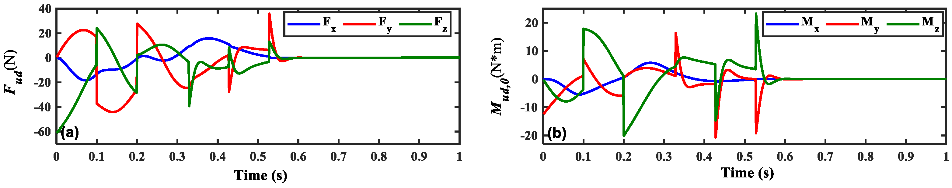
Figure 8.
The deviation curves of (a) , (b) , (c) , and (d) in the orbital coordinate system (te = 1.2 s).
Figure 8.
The deviation curves of (a) , (b) , (c) , and (d) in the orbital coordinate system (te = 1.2 s).
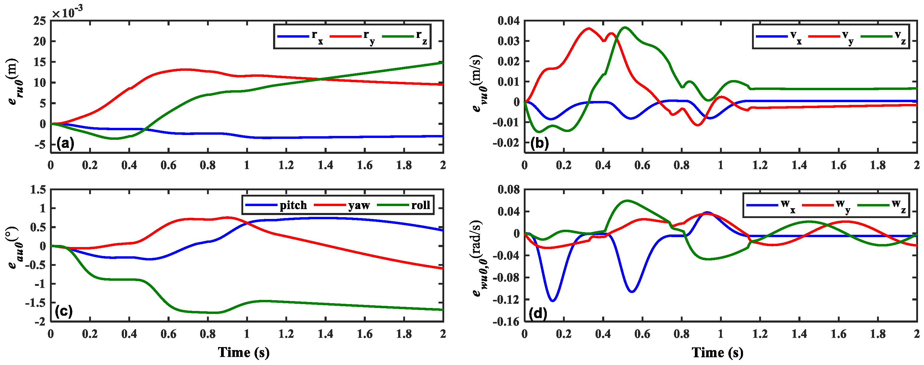
Figure 9.
The disturbance curves of (a) , (b) in the spinning satellite coordinate system (te = 0.4 s).
Figure 9.
The disturbance curves of (a) , (b) in the spinning satellite coordinate system (te = 0.4 s).
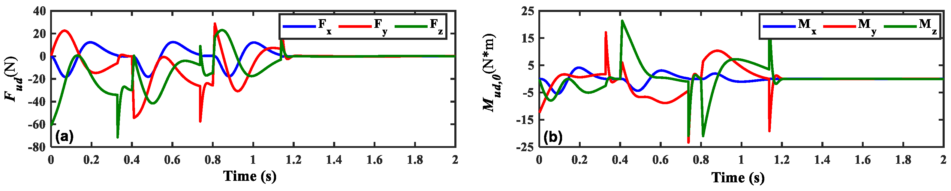
Figure 10.
The deviation curves of (a) , (b) , (c) , and (d) in the orbital coordinate system (te = 0.01 s).
Figure 10.
The deviation curves of (a) , (b) , (c) , and (d) in the orbital coordinate system (te = 0.01 s).
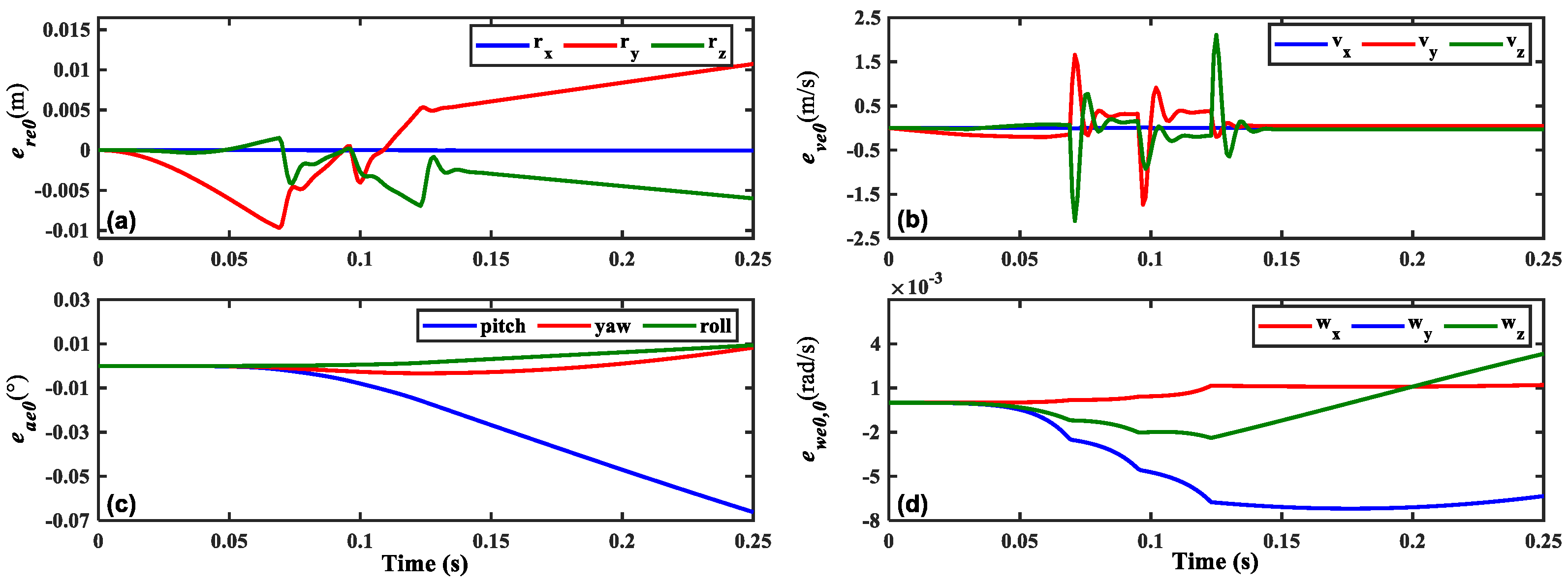
Figure 11.
The disturbance curves of (a) , (b) in the spinning satellite coordinate system (te = 0.01 s).
Figure 11.
The disturbance curves of (a) , (b) in the spinning satellite coordinate system (te = 0.01 s).
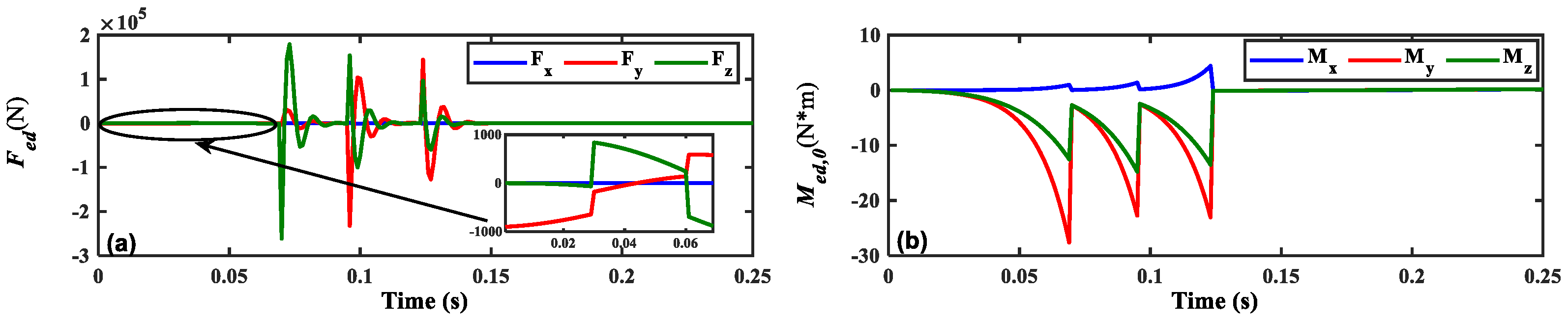
Figure 12.
The deviation curves of (a) , (b) , (c) , and (d) in the orbital coordinate system (te = 0.08 s).
Figure 12.
The deviation curves of (a) , (b) , (c) , and (d) in the orbital coordinate system (te = 0.08 s).

Figure 13.
The disturbance curves of (a) , (b) in the spinning satellite coordinate system (te = 0.08 s).
Figure 13.
The disturbance curves of (a) , (b) in the spinning satellite coordinate system (te = 0.08 s).

Table 1.
The parameter values of the spinning satellite with IPSs.
| Parameter | Description | Value |
|---|---|---|
| m0 | the mass of the spinning satellite | 150 kg |
| mk | the mass of the kth IPS | 2 kg |
| r0 | the displacement of the spinning satellite | [0 m 0 m 0 m]T |
| v0 | the velocity of the spinning satellite | [0 m/s 0 m/s 0 m/s]T |
| a0 | the Euler angle of the spinning satellite | [0° 0° 0°]T |
| w0,0 | the angular velocity of the spinning satellite | [10 rad/s 0.03 rad/s 0.03 rad/s]T |
| h | the height of the spinning satellite | 1.7 m |
| r | the radius of the spinning satellite | 0.6 m |
| the Euler angle of the kth IPS | 0° | |
| wk | the angular velocity of the kth IPS | 0 rad/s |
Table 2.
RMS comparison of calculation results of the finite element model and the proposed dynamic model.
Table 2.
RMS comparison of calculation results of the finite element model and the proposed dynamic model.
| Parameter | The Finite Element Model | The Proposed Dynamic Model |
|---|---|---|
| Fx | 74.5123 N | 72.2888 N (2.9841%) |
| Fy | 15,395 N | 14,895 N (3.2478%) |
| Fz | 18,063 N | 17,463 N (3.3217%) |
| Mx | 2.6426 N*m | 2.5355 N*m (4.0528%) |
| My | 6.2578 N*m | 6.0007 N*m (4.1084%) |
| Mz | 8.2648 N*m | 8.1714 N*m (1.1301%) |
Disclaimer/Publisher’s Note: The statements, opinions and data contained in all publications are solely those of the individual author(s) and contributor(s) and not of MDPI and/or the editor(s). MDPI and/or the editor(s) disclaim responsibility for any injury to people or property resulting from any ideas, methods, instructions or products referred to in the content. |
© 2023 by the authors. Licensee MDPI, Basel, Switzerland. This article is an open access article distributed under the terms and conditions of the Creative Commons Attribution (CC BY) license (https://creativecommons.org/licenses/by/4.0/).
Share and Cite
MDPI and ACS Style
Shang, Y.; Deng, Y.; Cai, Y.; Chen, Y.; He, S.; Liao, X.; Jiang, H. Modeling and Disturbance Analysis of Spinning Satellites with Inflatable Protective Structures. Aerospace 2023, 10, 971. https://doi.org/10.3390/aerospace10110971
AMA Style
Shang Y, Deng Y, Cai Y, Chen Y, He S, Liao X, Jiang H. Modeling and Disturbance Analysis of Spinning Satellites with Inflatable Protective Structures. Aerospace. 2023; 10(11):971. https://doi.org/10.3390/aerospace10110971
Chicago/Turabian StyleShang, Yuting, Yifan Deng, Yuanli Cai, Yu Chen, Sirui He, Xuanchong Liao, and Haonan Jiang. 2023. "Modeling and Disturbance Analysis of Spinning Satellites with Inflatable Protective Structures" Aerospace 10, no. 11: 971. https://doi.org/10.3390/aerospace10110971
Note that from the first issue of 2016, this journal uses article numbers instead of page numbers. See further details here.