
Multiple UAS Traffic Planning Based on Deep Q-Network with Hindsight Experience Replay and Economic Considerations


Mechanical Engineering Department, National University of Singapore, Singapore 117411, Singapore
*
Author to whom correspondence should be addressed.
Aerospace 2023, 10(12), 980; https://doi.org/10.3390/aerospace10120980
Submission received: 6 October 2023
/
Revised: 11 November 2023
/
Accepted: 13 November 2023
/
Published: 22 November 2023
(This article belongs to the Collection Air Transportation—Operations and Management)
Abstract
:This paper explores the use of deep reinforcement learning in solving the multi-agent aircraft traffic planning (individual paths) and collision avoidance problem for a multiple UAS, such as that for a cargo drone network. Specifically, the Deep Q-Network (DQN) with Hindsight Experience Replay framework is adopted and trained on a three-dimensional state space that represents a congested urban environment with dynamic obstacles. Through formalising a Markov decision process (MDP), various flight and control parameters are varied between training simulations to study their effects on agent performance. Both fully observable MDPs (FOMDPs) and partially observable MDPs (POMDPs) are formulated to understand the role of shaping reward signals on training performance. While conventional traffic planning and optimisation techniques are evaluated based on path length or time, this paper aims to incorporate economic analysis by considering tangible and intangible sources of cost, such as the cost of energy, the value of time (VOT) and the value of reliability (VOR). By comparing outcomes from an integration of multiple cost sources, this paper is better able to gauge the impact of various parameters on efficiency. To further explore the feasibility of multiple UAS traffic planning, such as cargo drone networks, the trained agents are also subjected to multi-agent point-to-point and hub-and-spoke network environments. In these simulations, delivery orders are generated using a discrete event simulator with an arrival rate, which is varied to investigate the effect of travel demand on economic costs. Simulation results point to the importance of signal engineering, as reward signals play a crucial role in shaping reinforcements. The results also reflect an increase in costs for environments where congestion and arrival time uncertainty arise because of the presence of other agents in the network.
1. Introduction
Modern-day consumerism rests on a foundation of a complex and interconnected global supply chain network. Online marketplaces and the promise of cheap and quick deliveries place immense stress on logistics networks, competing for scarce transport resources in an already congested environment. The pandemic has greatly exacerbated these issues by disabling workers and delaying shipments, leaving massive gaps in the system that send supply shocks through the economy.
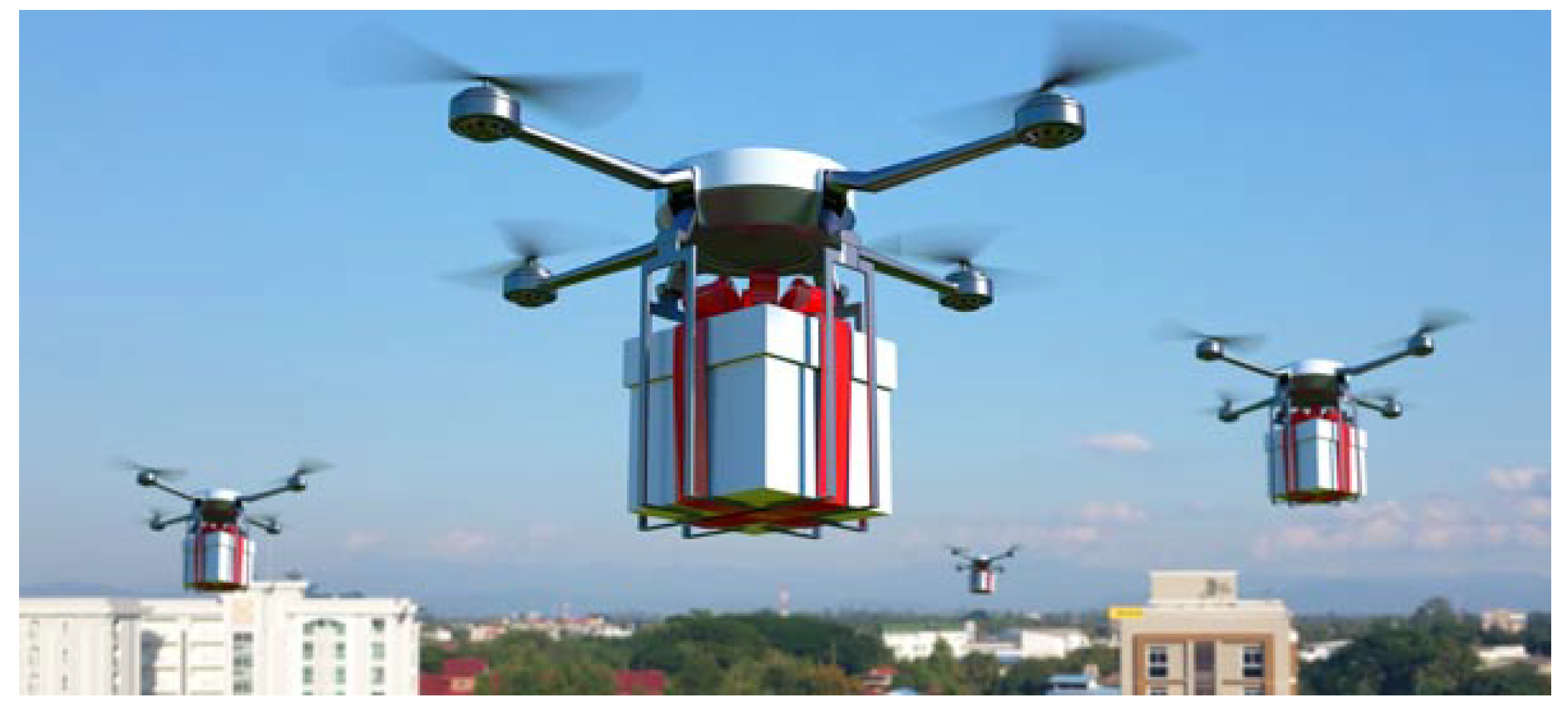
As road networks in densely populated urban areas are increasingly congested, the development of an aerial cargo drone network is a natural next step towards reducing the land-based last-mile delivery bottleneck, the journey from distribution warehouses to final users. An example is shown in Figure 1 [1]. With the airspace projected to be shared by a growing number of users, a fair and efficient traffic control system must, therefore, be adopted to ensure safe and continual operation.
Tall and often irregular structures in congested urban environments lead to many challenges in generating optimal traffic and individual aircraft trajectories. A conventional collision avoidance technique, such as a potential field (repulsive force for obstacles and attractive force for destination), takes a longer time to compute and may give a suboptimal solution. In addition, a collision avoidance manoeuvre is usually considered a convex optimisation problem, which may not be the case, and hence, the outcomes also depend on the initial guesses. The result can likewise be suboptimal. This also requires a certain computing time.
Reinforcement learning, however, surpasses other forms of control when individual agents following simple rules create systems that may not have easy closed-form analytical solutions. Despite each drone behaving within a well-defined set of dynamic and control parameters, the sheer number of combinations of sequential actions leads to an exponential growth of possibilities, analogous to the many different possible games and outcomes of chess. Only a sufficiently complex model trained on large sets of simulated data may possibly converge to an optimal solution.
Therefore, this paper explores the use of a technique in reinforcement learning known as the Deep Q-Network (DQN) to search for factors that lead to optimal drone traffic and individual trajectories. An analysis of economic costs across models trained on modified parameters also provides a sound understanding of these effects in different environments.
Because it is a relatively simple model, this Double Deep Q-Network with an experience replay model can also potentially be put into the onboard system of the drones for the real-world mission. The limitation is simply the connection and conjugation with the distance sensors and the communications with other drones.
Advantage of the Proposed Approach
While conventional traffic planning and optimisation techniques are evaluated based on path length or time, this paper incorporates economic analysis by considering tangible and intangible sources of cost, such as the cost of energy, the value of time (VOT) and the value of reliability (VOR). This is more practical and has a clear advantage over the conventional approach.
2. Literature Review
2.1. Graph Search for Path Planning
The path length is a useful heuristic for finding efficient aircraft trajectories. Graph networks model locations as nodes and distances as edges to solve for the shortest trajectory between two points. For instance, graph-based methods in the class of shortest path algorithms, such as Djikstra’s algorithm and the A* algorithm, use dynamic programming to iteratively search for the shortest path [2]. Tree-based methods, such as the rapidly-exploring random tree* (RRT*), on the other hand, circumvent the inefficiencies arising from random walks in graph-based searches by rapidly growing search trees far away [3].
However, several limitations of graph-based methods exist, with the most important being the assumption that the shortest path is equivalent to the most dynamically efficient path. Graph networks fail to consider the dynamic history of drones as they assign a fixed cost for traversals between adjacent nodes, whereas the current momentum and energy of these drones may alter these costs significantly. Drone networks are also expected to operate in relatively large environments, and the time complexities of graph-based algorithms do not scale well with the size or resolution of the search space. Therefore, other approaches to path planning need to be adopted instead.
2.2. Optimal Control
The modern approach to optimal control involves the formulation of a Bolza problem comprising an objective function of terminal and running cost components, and L, as shown in (1), which are minimised based on a dynamic constraint d, path constraint and boundary constraint [4]. The optimisation problem may be solved by using advanced numerical methods in non-linear programming, which is beyond the scope of this paper.
is subjected to
Unfortunately, most of these constrained optimisation problems are not analytically solvable and must be numerically solved for each problem through approximations or simulation-based methods, especially those of real-world problems. Furthermore, irregular state boundaries give rise to additional complexities in formulating solutions. Therefore, a new approach to solving optimal control problems is a better option.
2.3. Reinforcement Learning
Reinforcement learning allows agents with no prior information to learn an optimal policy through agent–environment interactions, without the need for retraining when new environments are encountered. The goal of reinforcement learning is to generate an optimal policy , representing the probability of taking an action a at each state s.
Deep Q-Networks arise from a combination of Q-learning and deep neural networks. Mnih et al. first used a DQN to train an agent to play several Atari 2600 computer games, with the agent performance surpassing all previously trained agents for six out of seven games and exceeding the level of an expert human player for three of them [5]. By iteratively computing expected future rewards using (2), known as the Bellman optimality equation, agents are trained to perform actions derived from a pre-determined policy (such as -greedy) according to the perceived cumulative discounted future reward of the state–action values generated by the trained neural network [6].
DQN is an off-policy algorithm that allows the neural network to be updated by Q-values of the subsequent state–action pair not derived from the actual policy. Such off-policy behaviour allows for better exploration and a faster convergence to an optimal path as compared with an on-policy algorithm, such as SARSA [7]. DQN also uses TD(0), a one-step lookahead temporal difference target, to update the neural network online, allowing for faster convergence than offline updating via whole Monte Carlo simulation episodes.
DQN has also been adopted to overcome the complexity of robot path planning. Raajan, et al. used a DQN in an environment with quantised agent states and both static and dynamic obstacles in the environment and compared it with traditional path planning algorithms, such as RRT* [8]. The results show a great improvement in computational time with little to no reduction in optimality, demonstrating the potential for deep reinforcement learning methods to explore decisions that go against the conventional intuition of heuristic-based approaches. Nevertheless, DQN has a computational overhead, and this can be a limiting factor in practical applications.
2.4. Transport Costs
Current path-finding algorithms are assessed based on the length of the shortest path between the origin and destination. While path length may be an important factor, there are other sources of economic costs that influence the optimal trajectory. These costs may be broadly categorised into tangible and intangible costs.
2.4.1. Tangible Costs
The tangible costs of operating a drone delivery service can be decomposed into fixed capital costs and variable operating costs. Fixed capital costs involve the initial capital required to initialise such a service, including the mechanical costs of constructing delivery drones, the infrastructure required for performing take-offs and landings and the regular maintenance costs required to maintain a fleet of drones. Since fixed costs are invariant across different control algorithms, they are beyond the focus of this paper.
Variable operating costs comprise several input costs that are dependent on the aggregate output of the drone service, quantifiable in terms of the total payload distance travelled. The seminal paper by D’Andrea estimates the power consumption for a cargo drone in (3), with as the payload mass in kg, as the vehicular mass in kg, g as the gravitational acceleration in m/s, v as the cruising velocity in m/s, as the dimensionless motor-propeller power transfer efficiency, as the dimensionless lift-to-drag ratio and as the power consumption for all other electronics in kW [9]. Using c as the cost of energy in dollars per kWh and e as the dimensionless charging efficiency, the cost per unit distance is also given by D’Andrea in (4).
Further studies have extended this model to include other factors that may affect the electric power required for different profiles of drone flight. A systematic review was conducted among extended models, accounting for variable weight profiles, different flight profiles and specific flight parameters, such as angle of attack, wind vectors and the various forces of flight [10].
2.4.2. Intangible Costs
Intangible costs are typically derivative of two sources: the value of time (VOT) and the value of reliability (VOR). The VOT refers to the willingness to pay to reduce the amount of travel time by one unit, and the VOR is the amount that a commuter is willing to pay to reduce a specified measure of uncertainty in arrival time by one unit.
In the case of physical commutes, Lam and Small estimated the VOT to be USD 22.87/h, and the VOR to be USD 15.12/h for males and USD 31.91/h for females [11]. The unit of uncertainty specified by Lam and Small is the difference between the 50th and 90th percentiles of the distribution of arrival timings, as there is typically little to no cost for arriving earlier than planned.
However, the applicability of commuter VOTs and VORs to last-mile drone deliveries may be weak. While there are numerous stated preference studies that estimate the VOT and VOR for passenger travel, there are few studies that focus on the domain of freight.
While there is no existing literature specific to cargo delivery drones, Shams examined the VOT and VOR for freight in the United States and produced estimates in [12] based on the mean time and the standard deviation of the distribution of arrival timings as unit measures. Fowkes also conducted a similar stated preference study in the United Kingdom but added controls for the values of early starts and late arrivals for freight transport [13]. The unit of uncertainty employed by Fowkes is the time difference between the earliest arrival and the 98th percentile of arrival. The results of both studies are presented in Table 1.
The following sections utilise and draw on these models to evaluate the effect of varying various hyperparameters on economic costs for an aerial cargo drone network.
3. Methodology
In this section, we briefly discuss the concept of the Deep Q-Network and Reward Engineering, specifically Hindsight Experience Replay. This is to understand our reinforcement learning approach. Subsequently, the setup environment and sample single- and multiple-agent traffic and individual path planning are presented.
3.1. Deep Q-Network (DQN)
As mentioned in the previous section (Reinforcement Learning), we employed Deep Q-Network as a tool. There are several excellent studies in the literature, such as Roderick et al. [14] and Fan et al. [15]. Here, we directly use the DQN Q-learning sampling-based method to find the future discounted value of taking an action a at a state s. A Q-table of dimension X is used to lookup the best action to take at every state s. The convergence through the Bellman optimality equation is shown in Equation (2).
The neural network is parameterised by parameter array , representing a series of weight matrices, and receives the state space input to produce an output action . With the large state space expected of the continuous environment, it is not feasible to store each action–value pair in a Q-table of dimension . Rather, a function approximator in the form of a deep neural network may be used to parameterise .
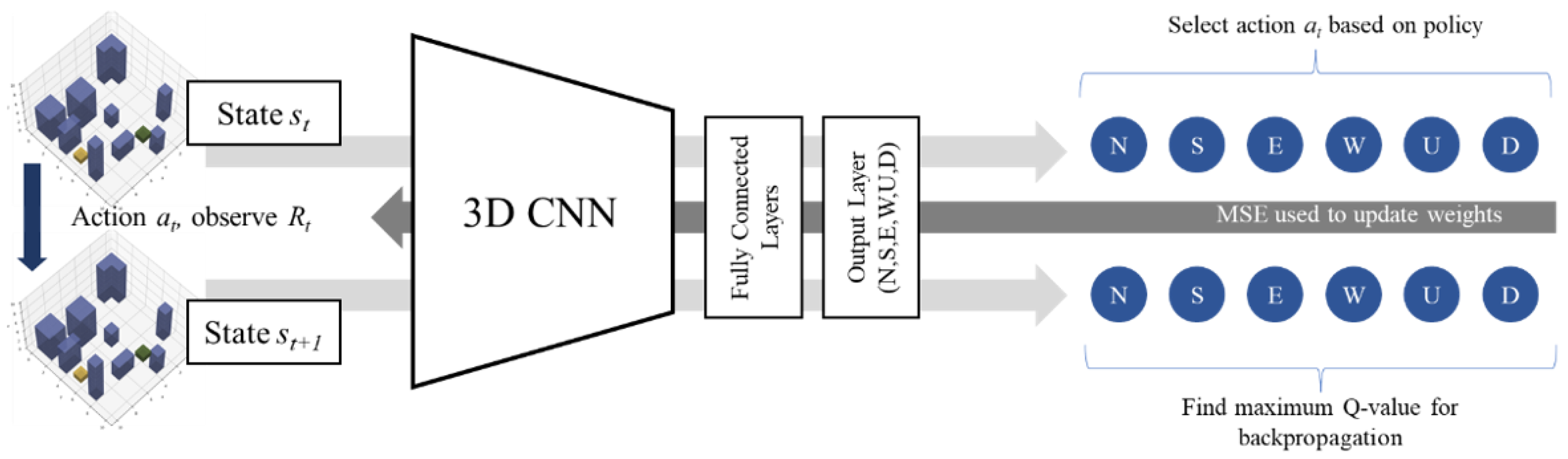
Since the environment is three-dimensional (3D), the state space is fed through a network of 3D convolution layers (3D-Conv) for feature extraction before passing through several fully connected hidden layers. By using a convolutional neural network (CNN), continuous and dynamic state spaces evolving over time are permitted since features of continuous terrain data may be extracted. Figure 2 shows how a CNN is incorporated into the DQN architecture. The model architectures used in this paper are specified in Appendix A.
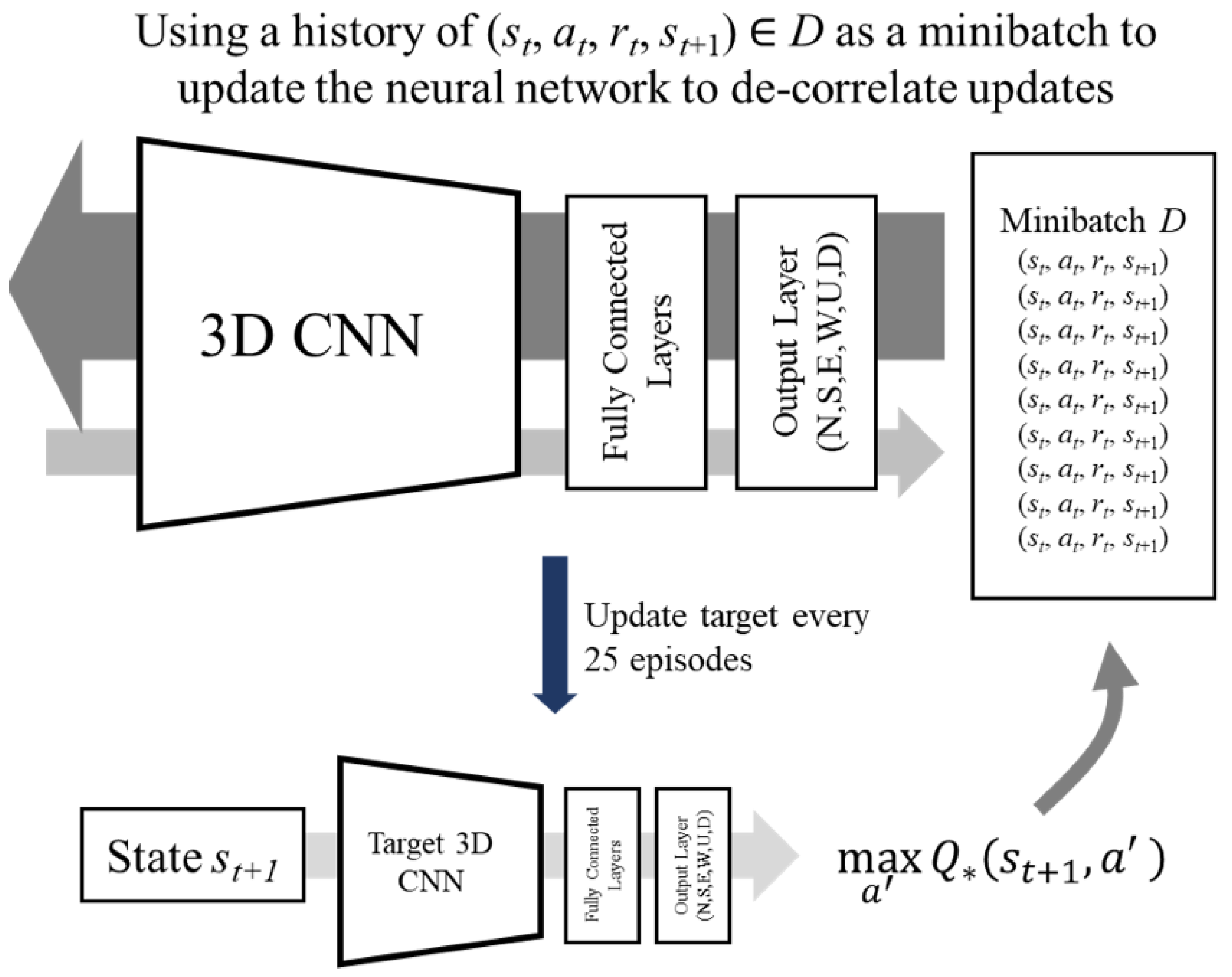
In dealing with the “deadly triad” of function approximation [16], temporal difference targets and off-policy learning, which may lead to a divergence in values [6], a modified DQN known as the Double DQN (DDQN) is used instead [17]. By obtaining Q-values from a secondary target network that is periodically updated from the primary network, action selection is decoupled from action evaluation, leading to better training stability. The DQN algorithm is adapted from van Hasselt et al. [17] and is presented in Algorithm 1. The corresponding schematic diagrams are available in Figure A1, Figure A2, Figure A3 and Figure A4 in Appendix A.
| Algorithm 1: Double Deep Q-Network with Experience Replay |
|
3.2. Reward Engineering
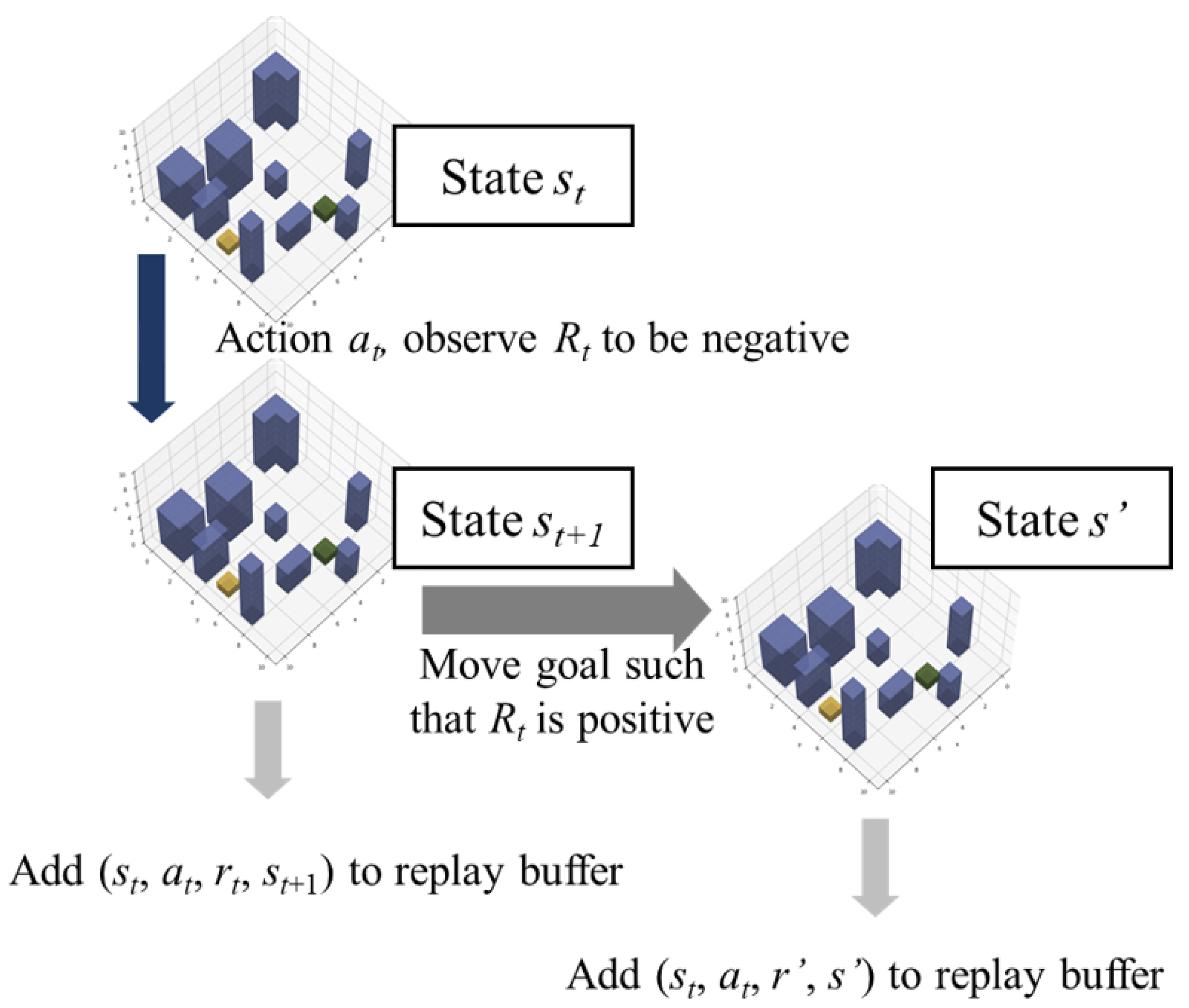
The objective of each agent is to navigate from its start state to its end state in the most efficient path possible, without the event of a collision. The reward function can be modelled as a signal from the environment, including the static or dynamic obstacles. With scarce positive rewards and abundant negative rewards in the MDP due to the presence of multiple obstacles in a congested urban environment, a lack of positive reinforcement may cause the agent to follow a suboptimal path that reduces the risk of terrain collision instead of converging toward the most efficient path. Therefore, a degree of reward engineering is necessary to improve the training paradigm. Current techniques in reward shaping involve heuristic inputs and may not be feasible for complex problems such as this. One novel technique involves the use of Hindsight Experience Replay (HER), an improvement to existing experience replay buffers by modifying the goal and the reward such that the frequency of positive reinforcement is increased [18]. This is done by shifting the goal state of the drone to its actual terminal state to simulate positive reward in certain replays, leading to additional simulated training examples that may be otherwise unattainable. The following Figure 3 and Figure 4 show the data movement and environment evolution for minibatch updating and Hindsight Experience Replay updating.
3.3. Environment
We specify the digitised environment as terrain or static obstacles and dynamic obstacles:
3.3.1. Urban Terrain/Static Obstacles
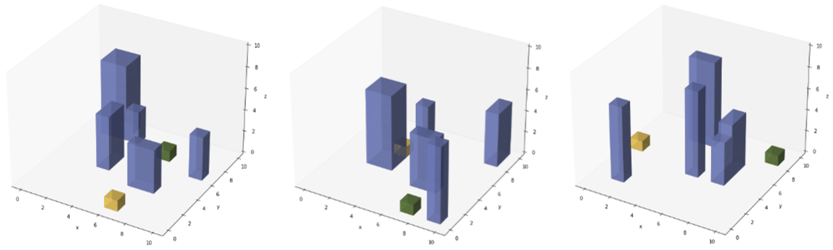
A random urban terrain generator is used to generate a simulated environment for model training. Each environment is initialised as empty, and B non-overlapping structures of various base shapes and heights are added to the terrain. The terrain is represented by three-dimensional voxels, with 0 used to represent empty space and 1 used to represent the presence of a built structure. Several samples are shown in Figure 5, with the yellow and green cubes representing the drone and goal, respectively.
3.3.2. Dynamic Obstacles
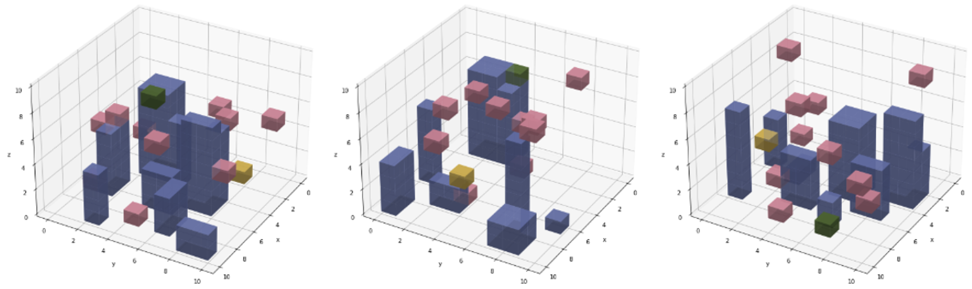
In addition to the static obstacles, D unit-sized dynamic obstacles, shown in pink in Figure 6, are also introduced to simulate other agents not controlled by the network. These agents follow a non-stationary, random walk with drift and Gaussian noise , as specified in (5).
3.3.3. Risks and Heterogenous Unit Step Cost
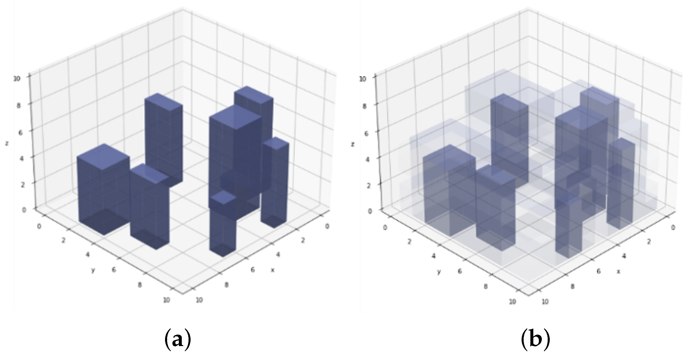
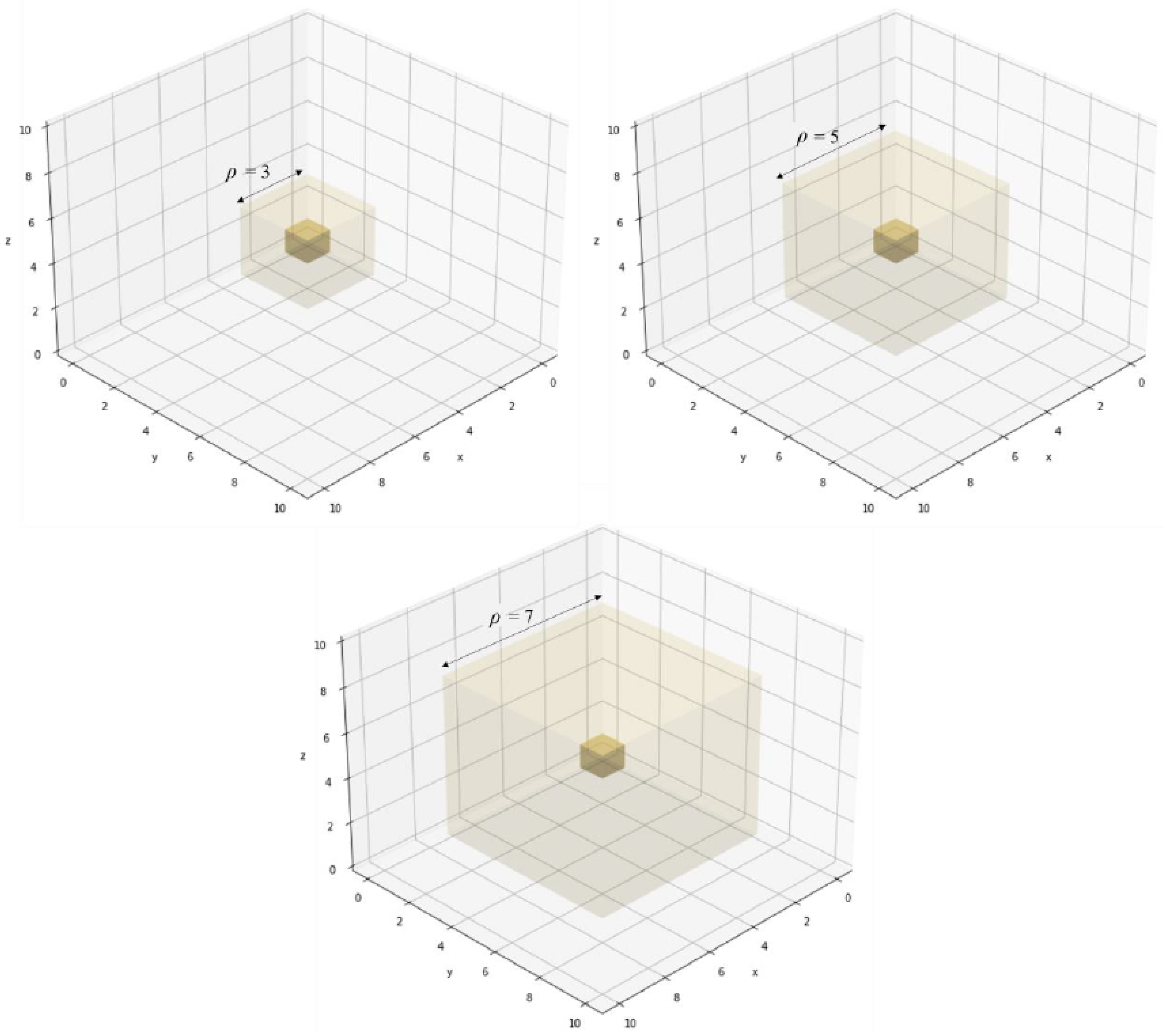
There are certainly inherent risks to operating aerial drone networks over populous and dense urban areas or areas with no navigational aids. Such risks are exogenous yet should reasonably affect the solution to the trajectory optimisation problem due to the immense negative externalities to life and infrastructure on the ground in the event of an accident. Therefore, the environment shall consider the risk associated with the occupancy of an agent in all valid spaces by assigning a value to the environment. These values manifest as state information to the agent to be learnt, resulting in a non-binary representation of the state s. The state information also modifies the reward space as a proportionate coefficient to the reward signal r that penalises traversally through risky regions. The level of risk associated with a particular location is represented by an equivalent degree of transparency in the respective spaces, as shown in Figure 7. This equivalent degree of transparency can also include the proximity to the infrastructure and the degree of visibility or occlusion within the navigation areas.
3.4. Single-Agent Path Planning
3.4.1. Fully Observable Markov Decision Process (MDP)
The single-agent drone path planning problem is first modelled as a fully observable Markov decision process (MDP) , which are defined as the following:
- : three-dimensional discrete state space;
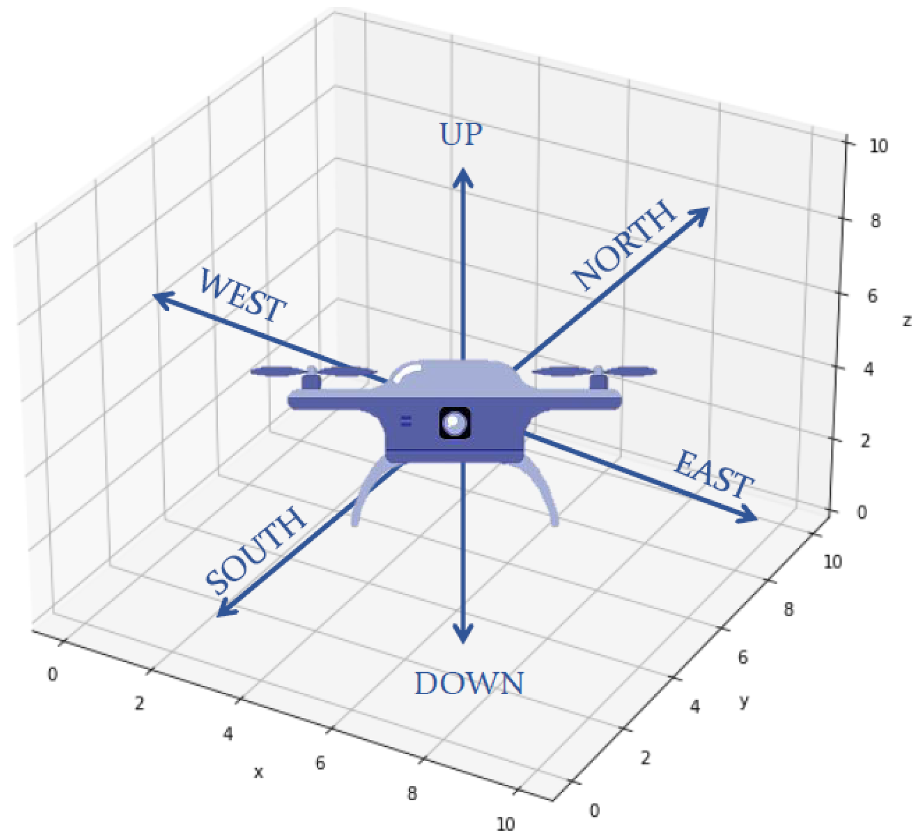
- : six possible actions corresponding to unit increments/decrements for each dimension (north, south, east, west, up, down); see Figure 8;
- : state transition matrix representing a probabilistic correspondence of each action; to a transition in , or ;
- : reward function as a signal from the environment to the agent for taking an action at a state and transitioning to state ;
- : discount factor to account for uncertainty in future rewards.
In this MDP, Table 2 specifies the variables . represents the deterministic kinematic transition a from state s to , without the presence of noise.
To understand the role of different environment characteristics and training paradigms on the performance on trained agents, a schedule of simulations in Table 3 is conducted. By varying one parameter between scheduled runs, the effect of that parameter on economic cost may be analysed under ceteris paribus conditions.
3.4.2. Partially Observable MDP
However, fully observable MDPs assume perfect and complete information, which may be an unrealistic assumption since the agent’s knowledge of the state is limited to the range of its onboard sensors. Complete information also increases the number of irrelevant dimensions for the agent to process when learning the optimal trajectory. Therefore, a partially observable MDP is formulated:
- : three-dimensional observation of the adjacent space with range , leading to an observed state of dimensions ;
- O: conditional observation that is deterministic conditional on .
For simplicity, the observation o is made deterministic given each state s, and the partially observable MDP is approximated as a fully observable MDP, with the state s set as the observable state . o is the extended Moore neighbourhood of range , a cube centred on the agent with length . Examples with varying are shown in Figure 9.
A separate schedule of simulations in Table 4 is conducted to study agent performance in partially observable MDPs and the effects of different observation distances.
3.5. Multiple-Agent Traffic and Individual-Path Planning
In operating a fleet network of drones, a fully observable MDP considers the exponentially complex action space of multiple agents. Therefore, this multiple-agent traffic planning problem considers independent agents operating within the same environment, each acting upon an observed state centred around their respective locations X. The formulated MDP is, therefore, reflective of the partially observable MDP as specified in the single-agent traffic planning problem. Each agent trains as a single agent but can thereafter be deployed as an independent agent in a multiple-agent system.
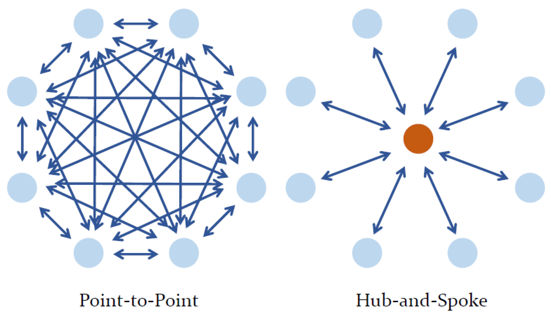
The performance of trained agents in the multiple-agent traffic and individual-path planning problem is assessed by simulating common airline network topologies. Cook and Goodwin outlined two prominent types of airline networks: point-to-point and hub-and-spoke systems [19] (see Figure 10), which may be used as multi-agent environments for agent evaluation.
3.5.1. Point-to-Point (P2P) Environment
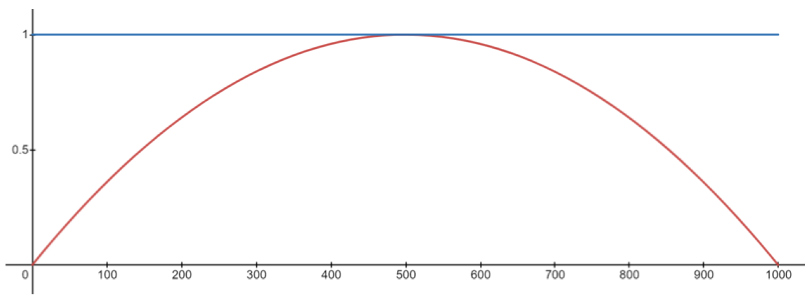
The most intuitive aerial transport network involves the direct routing of a drone from its origin to its destination via the shortest path. To simulate daily continuous operations, independent agents are generated with uniform spatial probability via a non-homogenous Poisson process with rate parameter specified in Equation (6). is a kernel function that can represent the aggregate demand for drone deliveries at time t. The shape of is given in Figure 11. Likewise, the intended destination of the drone is randomly generated.
Through varying the environment size, number of buildings, and the peak rate , the simulation schedule in Table 5 captures the effect of varying such parameters on agent performance. Each trained model in Section 3.2 tests on each of the scheduled runs.
3.5.2. Hub-and-Spoke Environment
The hub-and-spoke model is a widely adopted network topology that was popularised in the late 1970s, serving as an economically superior alternative to the existing P2P mode of civil air travel because of the ability to reap economics of density [19]. Likewise, the structure of modern-day logistics networks also resembles the hub-and-spoke model, as distributed payloads are agglomerated into a central arrival distribution hub, shipped to destination distribution hubs, and subsequently re-distributed to their respective destinations.
To assess the performance of trained agents serving as last-mile delivery services, a series of simulations in Table 6 with varying hubs and demands are performed. The equilibrium locations of H hubs of multiple delivery firms are hypothesised by Hotelling’s model of spatial competition [20], a dense cluster that is generated using a multivariable normal distribution centred at the centroid of the environment.
3.6. Performance Evaluation
Traditional approaches to optimal control minimise an objective function that comprises the path length and a heuristic representing control effort. However, an economic approach to cost is adopted, considering both tangible and intangible costs of operation for each drone delivery flight. This provides a more holistic perspective for cost–benefit analysis since the values of operations are quantified on an economic scale. The first type of costs is tangible resource costs. While the multitude of drone models available allows for much space to vary the parameters of flight, for the purposes of comparison, this methodology adopts conventional parameters that best represent the general population of cargo delivery drones. These parameters are fixed in Table 7.
Using (3) and (4), these drone and flight parameters give a total power consumption of 0.34525 kilowatts and a cost per unit distance p of 0.172625 US cents per kilometre. The other form of costs are intangible costs. The VOT estimates for freight transport are unlikely to apply in this context since the main opportunity costs of operating a vehicle for traditional freight shipping methods are inapplicable for an automated drone service. On the contrary, the concept of VOR is applicable to cargo delivery since there are costs to the consumer due to the uncertainty of package arrival timings. With a higher variance, consumers may need to plan around such uncertainty and, therefore, incur higher costs. For purposes of comparison against the various simulations, a value of USD 4.36 (2021 prices) is used as the monetary value associated with reducing the standard deviation of one ton of cargo drone delivery time by one hour [12]. With the parameters in Table 7, this corresponds to 1.308 US cents per hour of standard deviation. Despite the superiority of the 50th percentile to 90th percentile of arrival timings as a measure of VOR, this paper does not consider the use of this metric because of the unavailability of estimates for cargo deliveries.
4. Results
We ran the proposed Double Deep Q-Network with experience replay approach as shown in Algorithm 1 offline using an Intel I7 processor. All simulations were coded in the Python programming language, with the use of the Tensorflow Keras deep learning framework for model training, which was accelerated using the NVIDIA CUDA Deep Neural Network (cuDNN) package. The results from 1000 test simulations per model for single-agent FOMDPs presenting with the shortest path of minimum length equal to environment size N are presented in Table 8.
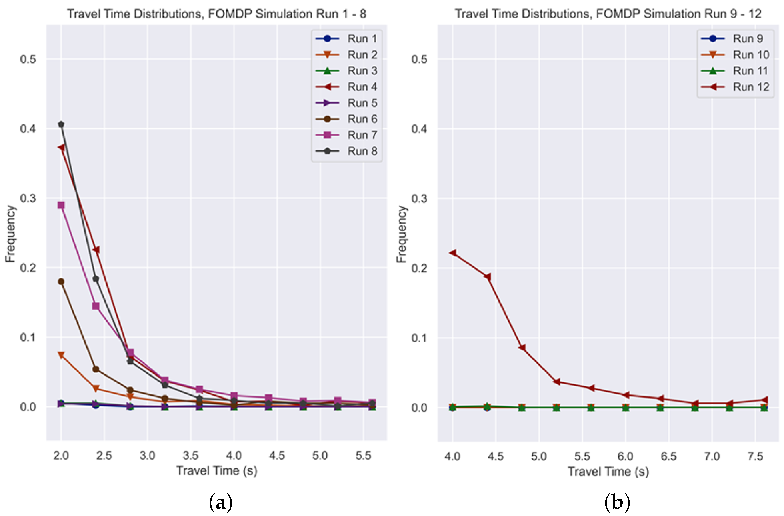
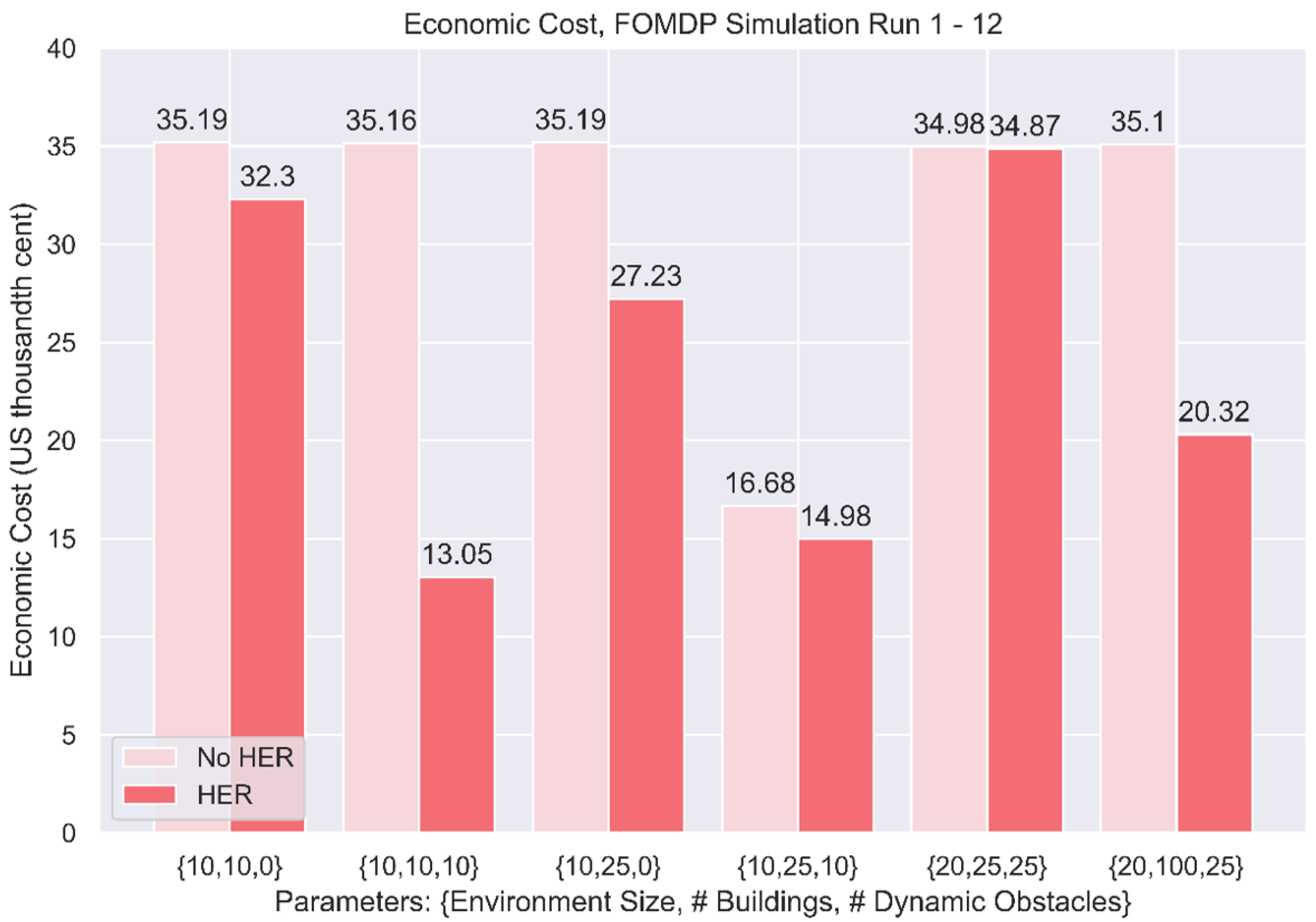
The graphs in Figure 12 present the test distribution of travel times for each trained agent, and Figure 13 shows the expected economic cost for Runs 1 to 12.
Likewise, the results from the single agent POMDP simulations for a fixed journey of length N are presented in Table 9.
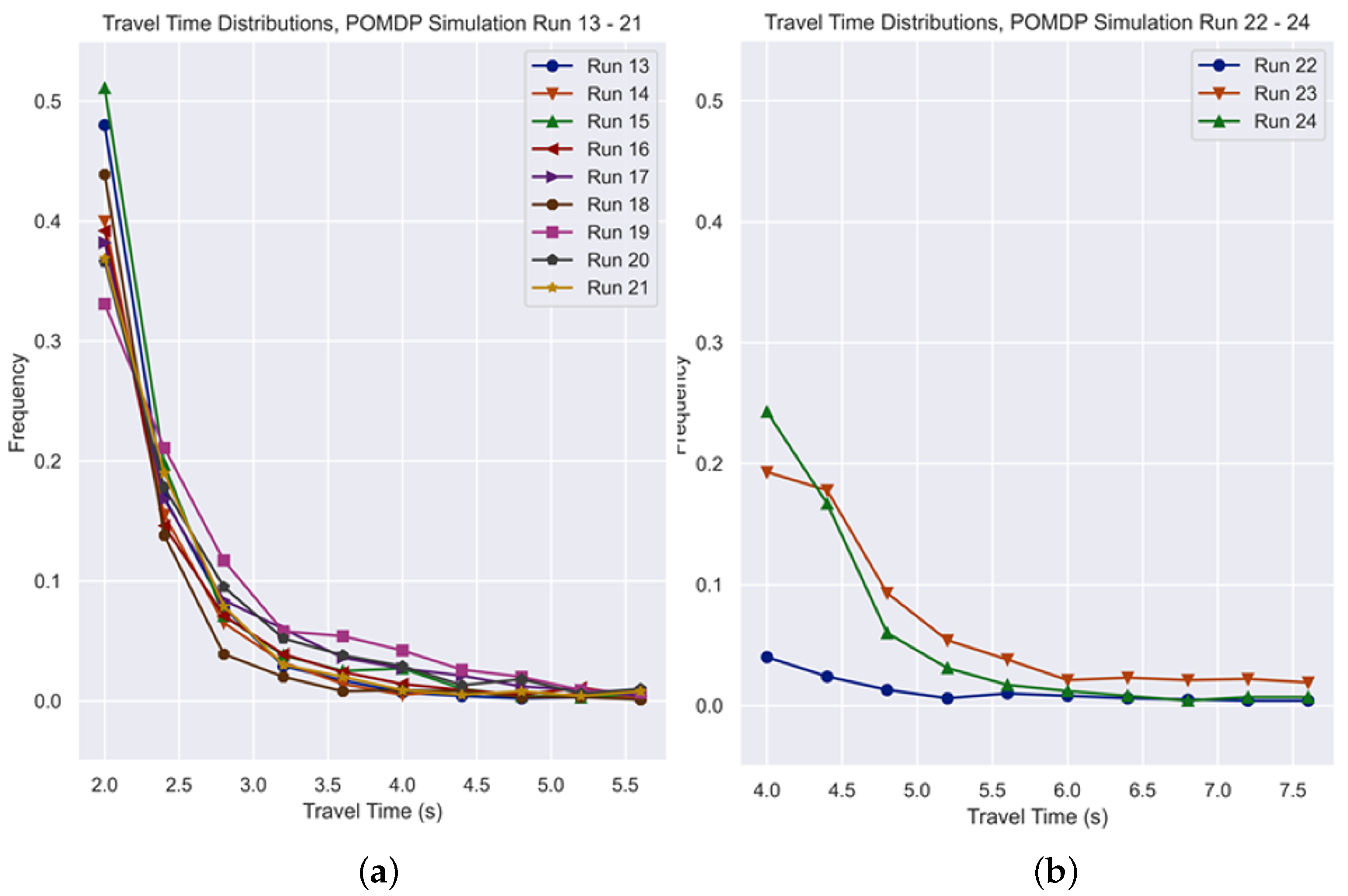
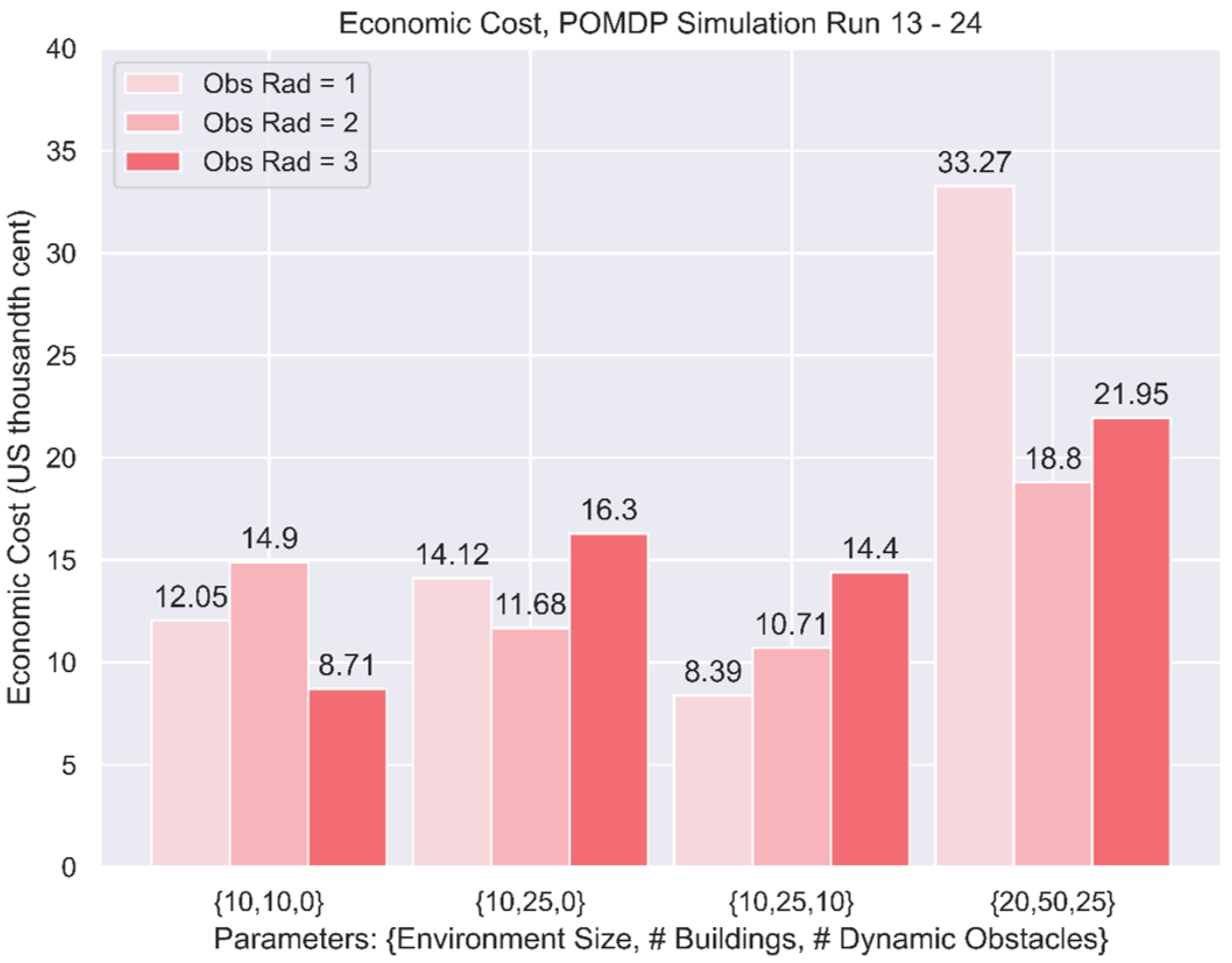
The graphs in Figure 14 present the test distribution of travel times for each trained agent, and Figure 15 shows the expected economic cost for Runs 13 to 24.
4.1. Point-to-Point Environment Test Results
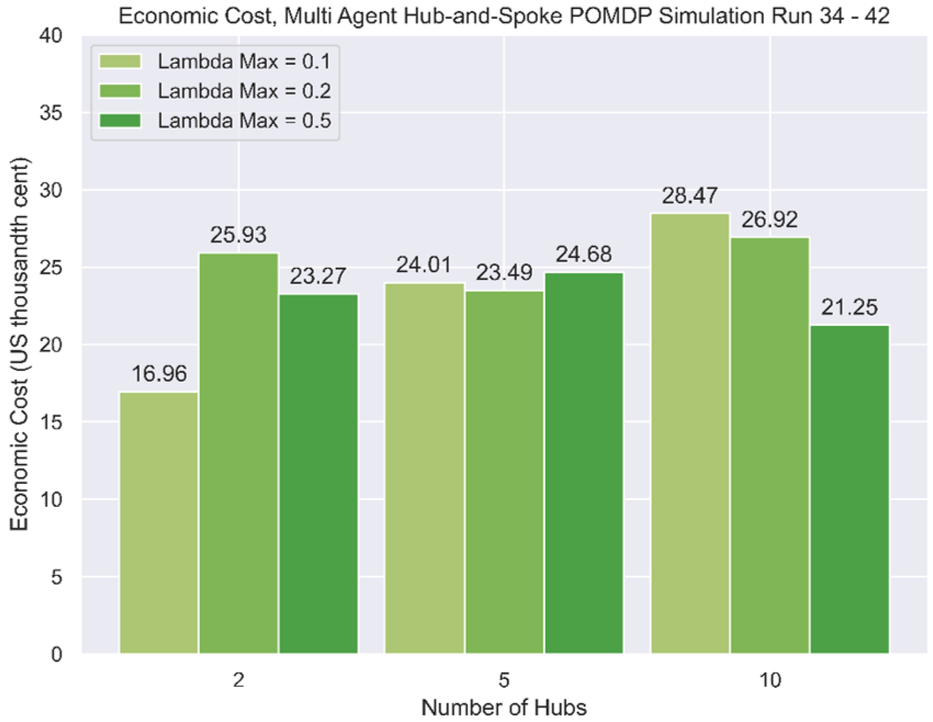
4.2. Hub-and-Spoke Environment Test Results
5. Discussion
5.1. Training Stability
In tuning the relevant hyperparameters of the DDQN, it was found that convergence to optimal values was not guaranteed, as shown by the results of several runs. Not all models reached convergence, with several simulations presenting rewards and travel times that are completely unusable, pointing to the delicate nature of training DQNs. This was supported by the theoretical instability of off-policy learning with bootstrapping and function approximation, with convergence achieved only with a sufficiently small learning rate and the discount factor . However, when these parameters were set to conservative values, the training regime stabilised, leading to overall better results. Nonetheless, the volatility of the resulting average reward curves results in the need to pick the optimal model based on the calculated training average reward, which is a certain overestimation of the model’s performance. Table 8 and Table 9 unequivocally point to the train-test gap of machine learning, which, therefore, requires a series of test simulations to assess the overall performance of the resultant models.
5.2. Signal Engineering
Prior to obtaining the results, it was hypothesised that a fully observable MDP would result in superior results to the partially observable MDP. Agents with perfect and complete information about the environment should result in more efficient outcomes because of the ability to learn the costs and benefits of taking a particular action. However, with POMDP models outperforming those with FOMDPs, it suggests that a degree of signal engineering may be required to guide the agent into learning an optimal strategy for its trajectory. There are several possible reasons that can be attributed to these observations. Firstly, it is well understood that the curse of dimensionality in statistical models, which refers to the high dimensionality of signal input into the model, may cause issues with learning if the signal-to-noise ratio is sufficiently small. The DDQN may pick up on unimportant features of the environment that may result in drastic changes to the output, especially given the instability of the TD targets, even in DDQN models where a target network is used. Secondly, placing the drone in the centre of its observed environment in the POMDP models, as compared to a delocalised environment in the FOMDP models, allows the agent to better learn the relative importance of spatial information in determining its next step. In spite of the universal approximation theorem, which allows sufficiently large neural networks the capability to learn the structure of any signal presented, it is likely necessary in practice to shape the state input to better assist the agent in identifying relevant features that will accelerate learning.
5.3. Effect of Hindsight Experience Replay
In the FOMDP simulations, the models trained with HER consistently performed better than the equivalent training regimes without HER, as underscored in Figure 8. HER strengthens the importance of handling scarce reward signals, a well-known problem in reinforcement learning that may cause training models to fail to converge because of a lack of positive reinforcement signals.
5.4. Effect of Dynamic Obstacles
Another surprising result is the consistent positive training effect of added dynamic obstacles to the environment. In both FOMDP and POMDP simulations, models with added dynamic obstacles tended to perform better, despite the added risk of collision. It is likely that these obstacles introduced a wider set of training examples into the CNN, giving the model a higher inclination to avoid actions that would lead to negative rewards.
5.5. Effect of Observation Radius
In the POMDP simulations with varying observation radius, there is no clear pattern from the results. However, it should be noted that the training of Run 22 did not converge well, suggesting that large environment sizes may require a certain degree of observation radius to train effectively. Nonetheless, there is insufficient evidence to support this claim definitively, and more tests should be conducted to ascertain the effect of observation radius on agent performance.
5.6. Effect of Travel Demand
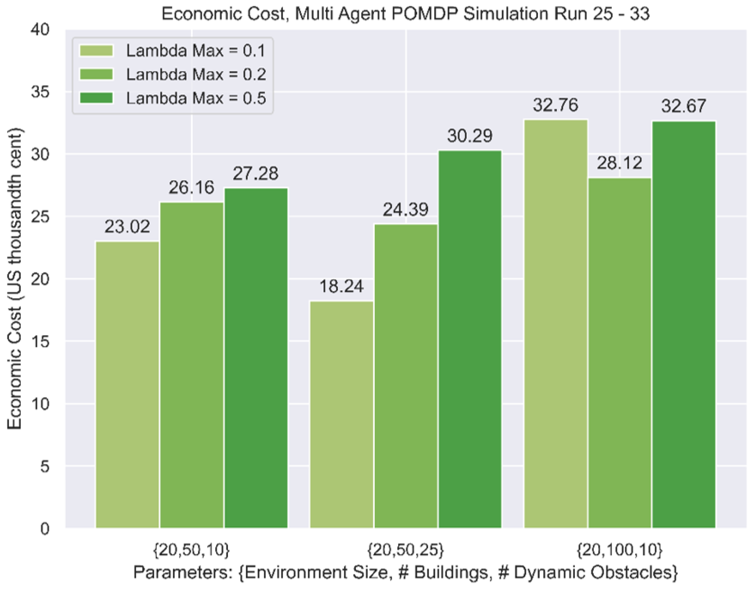
In varying the value of , which represents the maximum level of travel demand, the multi-agent simulations Run 25 to Run 30 reflected a higher economic cost because of the presence of congestion. However, the same effect was not observed from Run 31 to Run 33, which might be due to the high density of built structures. There was also no observable effect of demand on the hub-and-spoke environments.
5.7. Effect of Network Topology
A contrast between Figure 11 and Figure 12 is the effect of travel demand on economic costs. While the P2P environment suffered from inefficiencies arising from higher travel demand, there was less of a clear pattern for the hub-and-spoke environments. Intuitively, this could be due to the disruption of flow between two aircraft that were heading in opposing directions in the P2P environments, as compared to the hub-and-spoke networks, which facilitate largely unidirectional flow of traffic and are less prone to obstruction. However, these tests only simulated the outflow of cargo drones and did not consider inbound traffic. Further studies may be performed to ascertain the effects of bidirectional flow on economic efficiency.
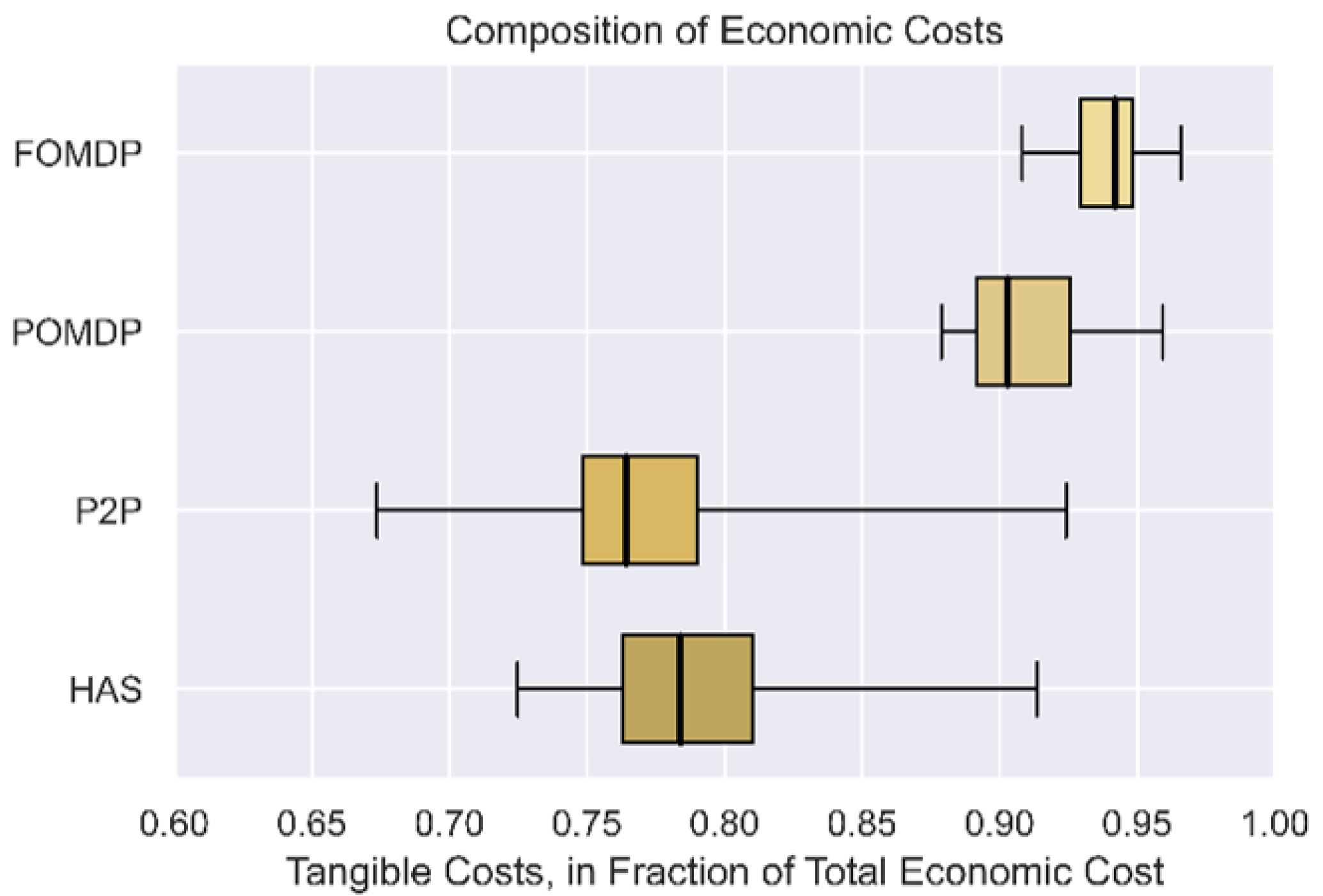
5.8. Proportion of Tangible and Intangible Costs
In all single-agent simulation tests, tangible costs accounted for 87% to 96% of total economic costs. However, the multiple agent tests reflected a lower percentage of 66% to 93%, as illustrated in Figure 18. This agrees with intuition as the level of travel time uncertainty rises in a multiple-agent environment, where multiple agents are competing for limited airspace, resulting in a higher tendency for congestion and a degree of unreliability. This cost structure does not include VOT and costs due to externalities, which may further reduce the proportion of tangible costs.
5.9. VOT and VOR Estimates
In calculating the expected economic costs for each aircraft trajectory, the VOT was assumed to be approximately zero, while the VOR was estimated from freight studies that may not be applicable to last-mile drone deliveries. Theoretically, the VOT for commuters comprises three components: the wage forgone, the dollar value of the utility gained from working, and the dollar value of the disutility gained from travel, as underlined in (7), where is the marginal utility per dollar of unearned income. However, in last-mile deliveries, there is no wage forgone by the recipient, and the work time is fixed since drone deliveries do not affect the work time of the consumer. Therefore, under certain assumptions, the VOT can potentially vary with delivery time if and only if there is an associated disutility gained from additional travel time.
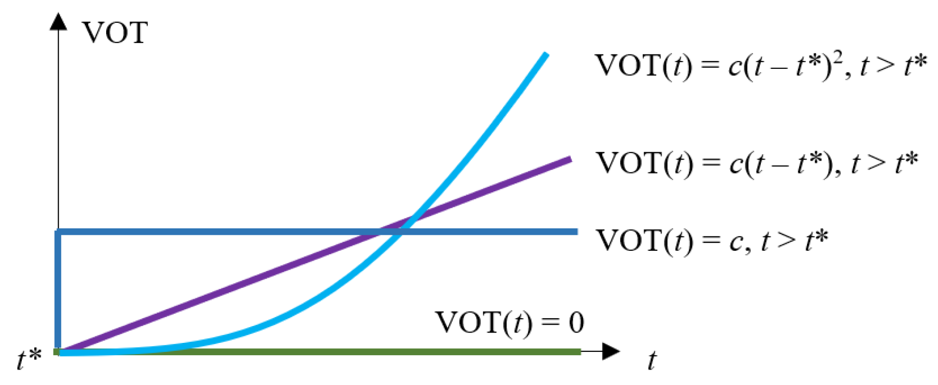
Goods that are time-sensitive may have a preferred time of arrival, , such that any arrival timing later than generates additional disutility to the consumer. On the other hand, if there is no urgency, there is no disutility generated from longer delivery times. While there is no definite study at present to estimate such numbers, a stated preference study may be conducted by giving consumers options for “Regular” and “Express” shipping as part of a choice set to measure the utility gained from earlier arrivals of different types of packages. As a result, different goods may have different VOT profiles for travel times after . Several candidate VOT profiles are shown in Figure 19.
Alternatively, a new framework for utility may be in order, given that the components of the utility function for cargo delivery may be significantly different from that for commuting. Morisugi developed separate utility specifications, which distinguished the case for non-business freight service, specifying a quality level indicator of freight time that decreases with time [21]. From solving the first-order conditions, the computed VOT is mathematically equivalent to the cost of freight service per freight time, p, multiplied by the time elasticity of , , as given in (8). By estimating the time elasticity of the quality of cargo drone deliveries, a more representative value of VOT for these purposes may be computed.
Intuitively, the VOR for delivery times is an important and significant component in the economic cost. Consumers often rely on expected arrival times to plan workflows that may be disrupted if these goods do not arrive at the expected arrival time. It is also important to acknowledge that the nature of the goods transported may widely affect these estimates since the ultimate value derived from the delivery time reliability may differ across various goods. More specifically, the interpretation of schedule delay early (SDE) and schedule delay late (SDL) costs can be extended into cargo deliveries. SDE costs may arise from additional storage costs due to early arrivals of goods, while SDL costs can accumulate from the potential cascading of delays and inconveniences due to late deliveries. Regardless, the assumed VOR structure is likely to be accurate because of the similarities underlying commuter travel and last-mile cargo deliveries.
5.10. Effect of Uncertainty of Data or Environment
As the proposed approaches depend largely on incoming sensing data and environmental input, the accuracy and reliability of the information may affect the performance of the approaches. Here, the effect of uncertainty due to the environment or sensing info comes in through signal input to the model. The current proposed approaches have two means to overcome this: (1) the use of probability in MDP as one of the inputs, which inherently covers the varying levels of uncertainty, and (2) the use of more training data with a variety of situations (and uncertainties). Hence, the variation of data has been taken care of, and the robustness of this method can be maintained.
6. Conclusions and Future Work
Through formulating an MDP using discrete three-dimensional space, this paper explores high-level control of aircraft trajectories for multi-agent traffic and path planning. The effects of various environment and flight parameters were analysed to calculate the impact on economic costs. However, these studies assumed a non-dynamical representation of the agent in the environment as they did not conform to dynamic and kinematic constraints. DQN also assumes a finite and discrete action space since the output layer of a neural network is discrete. These results may differ if a dynamic model of cargo drones with differentiated costs for the various actions is considered. For instance, the energy costs of ascending may be different from cruising or descending. Therefore, value-based learning methods can be further supported by policy gradient networks or actor-critic networks on more realistic models of cargo drones to derive more realistic estimates.
While conventional traffic planning and optimisation techniques are evaluated based on path length or time, this paper incorporates economic analysis by considering tangible and intangible sources of cost, such as the cost of energy, the value of time (VOT) and the value of reliability (VOR). This is more practical and has a clear advantage over the conventional approach.
More work is also required to study the VOT and VOR specific to cargo drone deliveries in congested urban areas. Present studies estimate freight VOT and VOR through containerised shipping methods that may not reflect the circumstances required for last-mile drone delivery. In measuring intangible costs, one of the major sources of externalities, noise pollution, may also be considered to reflect the total economic cost. It is reasonable to assume that the presence of flying aircraft in the vicinity of residential areas may cause unwanted disturbances that inflict external costs on society.
In addition, it must be acknowledged that these models only provide a high-level overview of multi-agent drone traffic, individual-path planning, and control. Other control models—not limited to those trained using reinforcement learning or neural networks—should also be developed to optimise the low-level actuator functions of cargo drones, in accompaniment to the policies that are established in this paper.
Furthermore, the proposed method can be scaled to large-scale networks by simply adding in the number of drones and the size of the environment in the training data, although there might be a limit due to the large computation involved.
Overall, the results from this paper show that the parameters that govern an aerial cargo drone network must be set correctly to maximise the efficiency of the network. This paper also demonstrates the usefulness of incorporating economic cost structures to an engineering-based problem. Such methods should continue to influence the analysis of engineering problems, especially where they are slated for implementation in society.
Author Contributions
Conceptualisation, S.X.S.; methodology, S.X.S. and S.S.; software, S.X.S.; validation, S.X.S. and S.S.; formal analysis, S.X.S. and S.S.; investigation, S.X.S. and S.S.; writing—original draft preparation, S.S.; writing—review and editing, S.X.S. and S.S.; project administration and funding, S.S. All authors have read and agreed to the published version of the manuscript.
Funding
This research received no external funding.
Conflicts of Interest
The authors declare no conflict of interest.
Abbreviations
The following abbreviations are used in this manuscript:
| A* | A-Star Pathfinding Algorithm |
| CNN | Convolutional Neural Network |
| CPI | Consumer Price Index |
| cuDNN | NVIDIA CUDA Deep Neural Network |
| DDQN | Double Deep Q-Networks |
| DQN | Deep Q-Networks |
| FOMDP | Fully Observable Markov Decision Process |
| HER | Hindsight Experience Replay |
| MDP | Markov Decision Process |
| P2P | Point-to-Point Multi-Agent Environment Model |
| POMDP | Partially Observable Markov Decision Process |
| RRT* | Rapidly-Exploring Random Tree Star Pathfinding Algorithm |
| SDE | Schedule Delay Early |
| SDL | Schedule Delay Late |
| TD(n) | Temporal Difference Target, n-step lookahead |
| VOR | Value of Reliability |
| VOT | Value of Time |
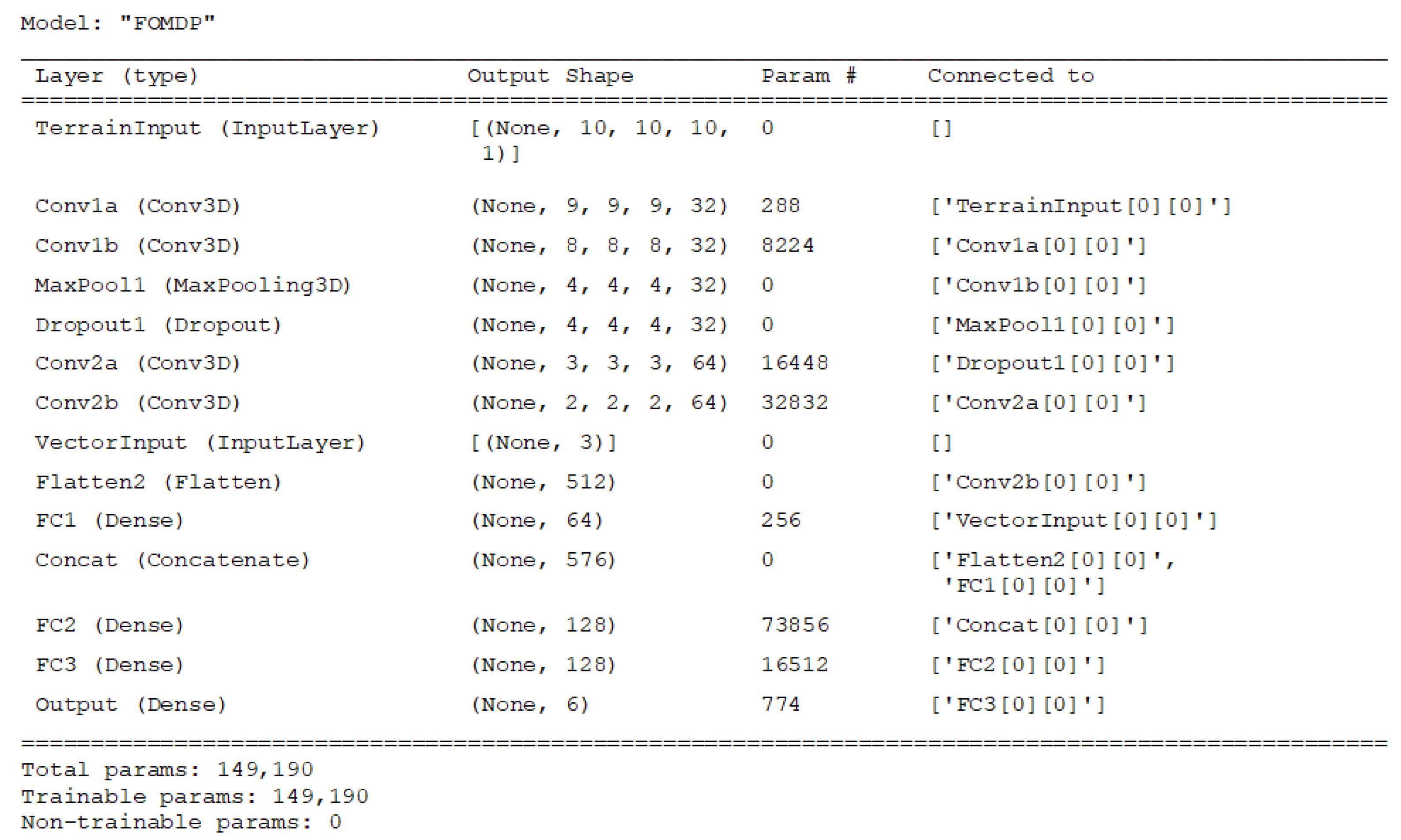
Appendix A. Model Architecture and Complexity
Details of the two model architectures used for training in the FOMDP and POMDP simulations are given in the following descriptors and schematics in Figure A1, Figure A2, Figure A3 and Figure A4.
Figure A1.
Description of CNN-DQN model for FOMDP simulations.

Figure A2.
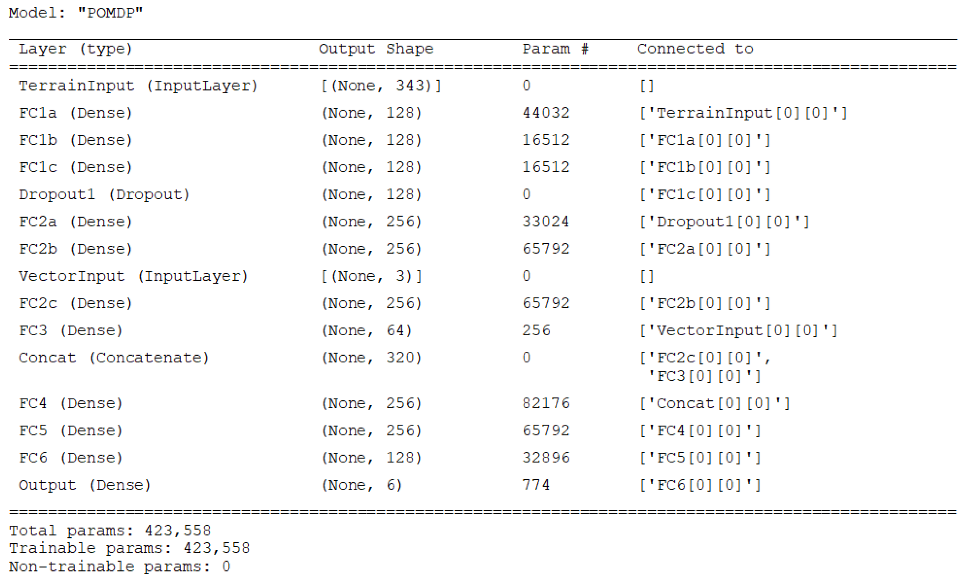
Description of CNN-DQN model for POMDP simulations.

Figure A3.
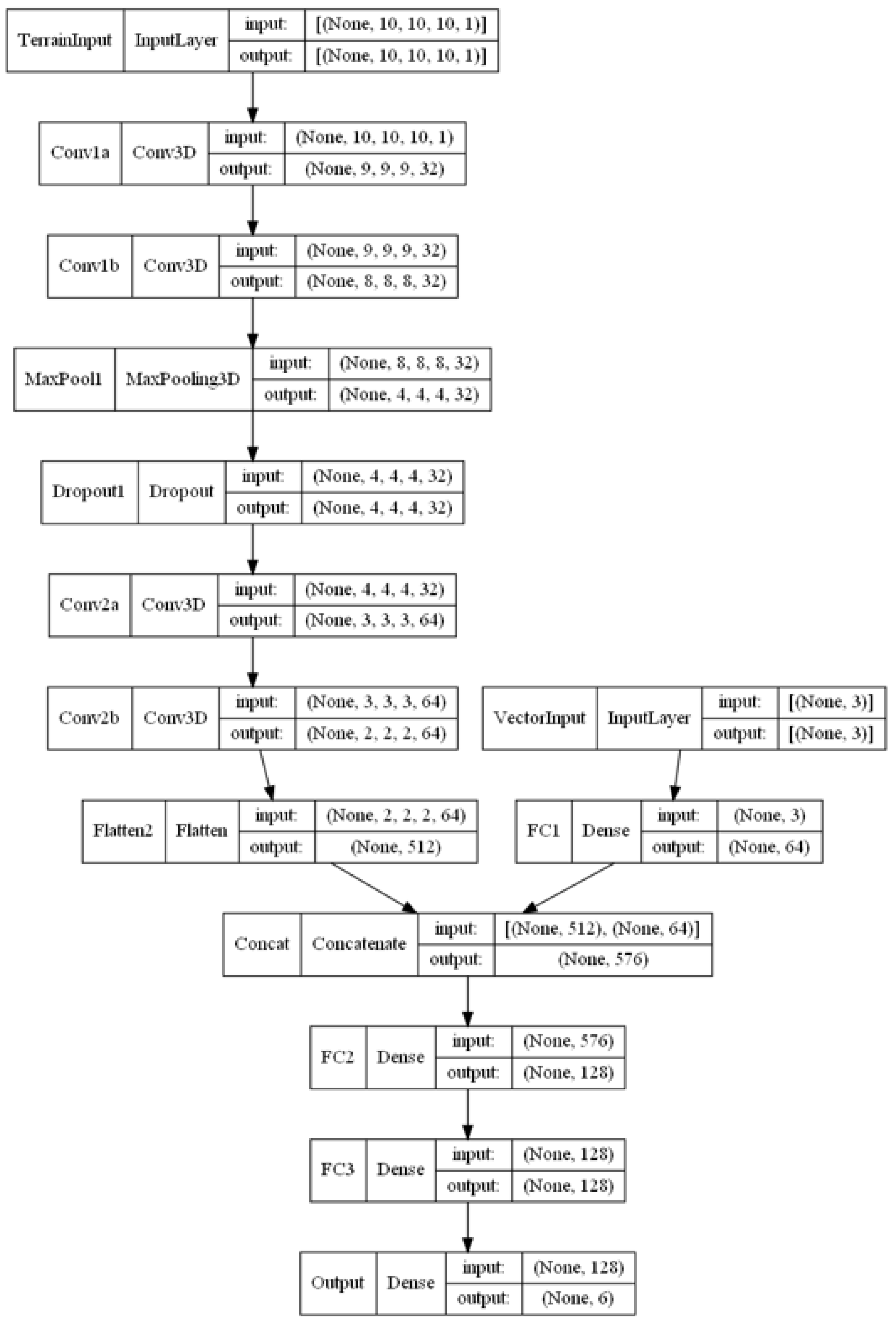
CNN-DQN schematic for FOMDP with input size (10,10,10),3..

Figure A4.
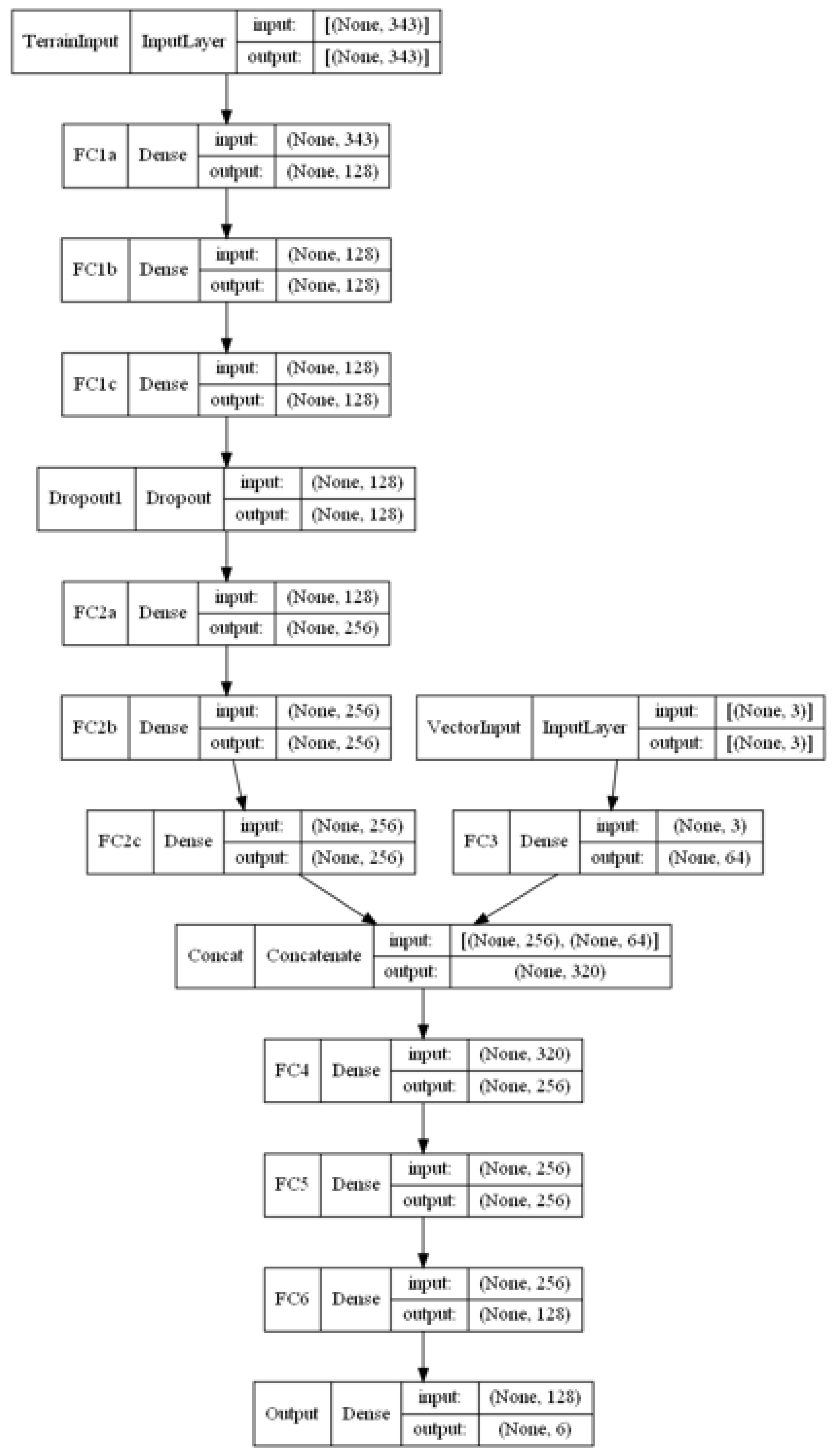
CNN-DQN schematic for POMDP with input size 343,3..

References
- Unmanned Airspace, Unmanned Air System Traffic Management (UTM). 2023. Available online: https://www.unmannedairspace.info/unmanned-air-system-traffic-management-utm-directory/ (accessed on 30 September 2023).
- Hart, P.E.; Nilsson, N.J.; Raphael, B. A formal basis for the heuristic determination of minimum cost paths. IEEE Trans. Syst. Sci. Cybern. 1968, 4, 100–107. [Google Scholar] [CrossRef]
- Karaman, S.; Frazzoli, E. Incremental sampling-based algorithms for optimal motion planning. Robot. Sci. Syst. VI 2010, 104, 267–274. [Google Scholar]
- Bliss, G.A. The problem of Bolza in the calculus of variations. In Annals of Mathematics; Mathematics Department, Princeton University: Princeton, NJ, USA, 1932; pp. 261–274. [Google Scholar]
- Mnih, V.; Kavukcuoglu, K.; Silver, D.; Graves, A.; Antonoglou, I.; Wierstra, D.; Riedmiller, M. Playing atari with deep reinforcement learning. arXiv 2013, arXiv:1312.5602. [Google Scholar]
- Sutton, R.S.; Barto, A.G. Reinforcement Learning: An Introduction; MIT Press: Cambridge, MA, USA, 2018. [Google Scholar]
- Sutton, R.S.; McAllester, D.; Singh, S.; Mansour, Y. Policy gradient methods for reinforcement learning with function approximation. Adv. Neural Inf. Process. Syst. 1999, 12, 1057–1063. [Google Scholar]
- Raajan, J.; Srihari, P.; Satya, J.P.; Bhikkaji, B.; Pasumarthy, R. Real Time Path Planning of Robot using Deep Reinforcement Learning. IFAC-PapersOnLine 2020, 53, 15602–15607. [Google Scholar] [CrossRef]
- D’Andrea, R. Can Drones Deliver? Automation Science and Engineering. IEEE Trans. 2014, 11, 647–648. [Google Scholar]
- Zhang, J.; Campbell, J.F.; Sweeney, D.C., II; Hupman, A.C. Energy consumption models for delivery drones: A comparison and assessment. Transp. Res. Part D Transp. Environ. 2021, 90, 102668. [Google Scholar] [CrossRef]
- Lam, J.; Bai, X. Transportation Research Part E. Logist. Transp. Rev. 2016, 16, 27. [Google Scholar]
- Shams, Kollol, Understanding the Value of Travel Time Reliability for Freight Transportation to Support Freight Planning 2016. Available online: https://digitalcommons.fiu.edu/etd/2828/ (accessed on 30 September 2023).
- Fowkes, T. The design and interpretation of freight stated preference experiments seeking to elicit behavioural valuations of journey attributes. Transp. Res. Part B Methodol. 2007, 41, 966–980. [Google Scholar] [CrossRef]
- Roderick, M.; MacGlashan, J.; Tellex, S. Implementing the deep q-network. arXiv 2017, arXiv:1711.07478. [Google Scholar]
- Fan, J.; Wang, Z.; Xie, Y.; Yang, Z. A theoretical analysis of deep Q-learning. In Proceedings of the 2nd Conference on Learning for Dynamics and Control, PMLR, Berkeley, CA, USA, 10–11 June 2020; pp. 486–489. [Google Scholar]
- Van Hasselt, H.; Doron, Y.; Strub, F.; Hessel, M.; Sonnerat, N.; Modayil, J. Deep reinforcement learning and the deadly triad. arXiv 2018, arXiv:1812.02648. [Google Scholar]
- Van Hasselt, H.; Guez, A.; Silver, D. Deep reinforcement learning with double q-learning. In Proceedings of the AAAI Conference on Artificial Intelligence, Phoenix, AZ, USA, 12–17 February 2016; Volume 30. [Google Scholar]
- Andrychowicz, M.; Wolski, F.; Ray, A.; Schneider, J.; Fong, R.; Welinder, P.; McGrew, B.; Tobin, J.; Pieter Abbeel, O.; Zaremba, W. Hindsight experience replay. Adv. Neural Inf. Process. Syst. 2017, 30. [Google Scholar]
- Cook, G.N.; Goodwin, J. Airline networks: A comparison of hub-and-spoke and point-to-point systems. J. Aviat./Aerosp. Educ. Res. 2008, 17. [Google Scholar] [CrossRef]
- Harold, H. Stability in competition. Econ. J. 1929, 39, 41–57. [Google Scholar]
- Morisugi, H. Measurement of Value of Time for Freight Trips and its Benefit by Market Information. Transp. Res. Procedia 2017, 25, 5144–5159. [Google Scholar] [CrossRef]
Figure 1.
Sample multiple cargo drone traffic [1].
Figure 1.
Sample multiple cargo drone traffic [1].

Figure 2.
CNN-DQN model architecture and training regime.

Figure 3.
Algorithm schematic for training with replay buffers.

Figure 4.
Algorithm schematic for HER updates.

Figure 5.
Sample urban terrain with drone locations and end goal locations.

Figure 6.
Sample urban terrain with added dynamic obstacles, highlighted in pink.

Figure 7.
Exogenous risk models. (a) Uniform step cost. (b) Heterogenous risk costs.

Figure 8.
Six possible actions corresponding to unit increments/decrements for each dimension (north, south, east, west, up, down).
Figure 8.
Six possible actions corresponding to unit increments/decrements for each dimension (north, south, east, west, up, down).

Figure 9.
Varying observable radius of agent in partially observable MDP in the extended Moore neighbourhood of range .
Figure 9.
Varying observable radius of agent in partially observable MDP in the extended Moore neighbourhood of range .

Figure 10.
Point-to-point and hub-and-spoke systems [19].
Figure 10.
Point-to-point and hub-and-spoke systems [19].

Figure 11.
Poisson process rate parameter with T = 1000 and = 1.

Figure 12.
Travel time distributions. (a) Runs 1 to 8, with environment size = path length = 20 m. (b) Runs 9 to 12, with environment size = path length = 40 m.
Figure 12.
Travel time distributions. (a) Runs 1 to 8, with environment size = path length = 20 m. (b) Runs 9 to 12, with environment size = path length = 40 m.

Figure 13.
Summary of economic costs, FOMDP, single agent.

Figure 14.
Travel time distributions. (a) Runs 13 to 21, with environment size = path length = 20 m. (b) Runs 22 to 24, with environment size = path length = 40 m.
Figure 14.
Travel time distributions. (a) Runs 13 to 21, with environment size = path length = 20 m. (b) Runs 22 to 24, with environment size = path length = 40 m.

Figure 15.
Summary of economic costs, POMDP, single agent.

Figure 16.
Summary of economic costs, P2P environment, multiple agents.

Figure 17.
Summary of economic costs, hub-and-spoke environment, multiple agents.

Figure 18.
Tangible costs as a fraction of economic costs, all simulations.

Figure 19.
Different VOT profiles for different goods.


Table 1.
Estimates for VOT and VOR for freight.
| Type of Goods | VOT | VOT | VOR | VOR |
|---|---|---|---|---|
| (USD/ton-h) | (USD/ton-h) | (USD/ton-h) | USD/ton-h) | |
| [12] | [13] | [12] | [13] | |
| Perishable | 0.71 | 0.49–0.84 | 4.95 | 0.65–4.82 |
| Non-perishable | 1.61 | 0.49–0.84 | 3.55 | 0.65–4.82 |
Table 2.
MDP specifications.
| Variables | Specifications (Set as Hyperparameters) |
|---|---|
| , for | |
| , for , , | |
| , otherwise | |
| , for successful delivery | |
| , for heterogenous unit step cost, | |
| , for collision | |
| 0.95 |
Table 3.
Fully observable MDP simulation schedule.
| Run | Environment Size, | # Buildings, B | # Dynamic Obstacles, | Hindsight Experience Replay |
|---|---|---|---|---|
| 1 | 10 | 10 | 0 | No |
| 2 | 10 | 10 | 0 | Yes |
| 3 | 10 | 10 | 10 | No |
| 4 | 10 | 10 | 10 | Yes |
| 5 | 10 | 25 | 0 | No |
| 6 | 10 | 25 | 0 | Yes |
| 7 | 10 | 25 | 10 | No |
| 8 | 10 | 25 | 10 | Yes |
| 9 | 20 | 50 | 25 | No |
| 10 | 20 | 50 | 25 | Yes |
| 11 | 20 | 100 | 25 | No |
| 12 | 20 | 100 | 25 | Yes |
Table 4.
Partially observable MDP simulation schedule.
| Run | Environment Size, | # Buildings, B | # Dynamic Obstacles, | Observable Radius, |
|---|---|---|---|---|
| 13 | 10 | 10 | 0 | 1 |
| 14 | 10 | 10 | 0 | 2 |
| 15 | 10 | 10 | 0 | 3 |
| 16 | 10 | 25 | 0 | 1 |
| 17 | 10 | 25 | 0 | 2 |
| 18 | 10 | 25 | 0 | 3 |
| 19 | 10 | 25 | 10 | 1 |
| 20 | 10 | 25 | 10 | 2 |
| 21 | 10 | 25 | 10 | 3 |
| 22 | 20 | 50 | 25 | 1 |
| 23 | 20 | 50 | 25 | 2 |
| 24 | 20 | 50 | 25 | 3 |
Table 5.
Point-to-point multi-agent simulation schedule.
| Run | Environment Size, | # Buildings, B | # Dynamic Obstacles, | |
|---|---|---|---|---|
| 25 | 20 | 50 | 10 | 0.1 |
| 26 | 20 | 50 | 10 | 0.2 |
| 27 | 20 | 50 | 10 | 0.5 |
| 28 | 20 | 50 | 25 | 0.1 |
| 29 | 20 | 50 | 25 | 0.2 |
| 30 | 20 | 50 | 25 | 0.5 |
| 31 | 20 | 100 | 25 | 0.1 |
| 32 | 20 | 100 | 25 | 0.2 |
| 33 | 20 | 100 | 25 | 0.5 |
Table 6.
Hub-and-spoke multi-agent simulation schedule.
| Run | Environment Size, | # Buildings, B | # Dynamic Obstacles, | # Hubs | |
|---|---|---|---|---|---|
| 34 | 20 | 50 | 25 | 2 | 0.1 |
| 35 | 20 | 50 | 25 | 2 | 0.2 |
| 36 | 20 | 50 | 25 | 2 | 0.5 |
| 37 | 20 | 50 | 25 | 5 | 0.1 |
| 38 | 20 | 50 | 25 | 5 | 0.2 |
| 39 | 20 | 50 | 25 | 5 | 0.5 |
| 40 | 20 | 50 | 25 | 10 | 0.1 |
| 41 | 20 | 50 | 25 | 10 | 0.2 |
| 42 | 20 | 50 | 25 | 10 | 0.5 |
Table 7.
Drone parameters.
| Parameter | Value |
|---|---|
| Mass of payload, (kg) | 2.0 |
| Mass of vehicle, (kg) | 3.0 |
| Unit Step Size, (m) | 2.0 |
| Unit Time, (s) | 0.2 |
| Constant Velocity, (m/s) | 10 |
| Lift-to-drag Ratio, | 4.0 |
| Power Transfer Efficiency, | 0.5 |
| Avionics Power, (kW) | 0.1 |
| Cost of Electric Power, (USD/kWh) | 0.144 |
| Cost of Electric Power, c (USD/kWs) | 0.00004 |
| Charging Efficiency, e | 0.8 |
Table 8.
Fully Observable MDP simulation results.
| Run | Parameters [, HER] | Training Reward | Test Reward | Mean Time () | Time S.D. () | Economic Cost (US Cents) |
|---|---|---|---|---|---|---|
| 1 | [10, 10, 0, N] | −0.640 | −1.010 | 20.051 | 1.592 | 0.03519 |
| 2 | [10, 10, 0, Y] | 0.137 | −0.918 | 17.413 | 6.168 | 0.03230 |
| 3 | [10, 10, 10, N] | −0.490 | −1.427 | 19.9476 | 2.009 | 0.03516 |
| 4 | [10, 10, 10, Y] | 0.755 | 0.403 | 6.144 | 6.730 | 0.01305 |
| 5 | [10, 25, 0, N] | −0.13 | −0.992 | 20.020 | 1.733 | 0.03519 |
| 6 | [10, 25, 0, Y] | 0.148 | −0.674 | 14.096 | 7.985 | 0.02723 |
| 7 | [10, 25, 10, N] | 0.151 | 0.173 | 8.074 | 7.548 | 0.01668 |
| 8 | [10, 25, 10, Y] | 0.716 | 0.190 | 7.082 | 7.576 | 0.01498 |
| 9 | [20, 50, 25, N] | −0.430 | −1.560 | 20.188 | 0.354 | 0.03498 |
| 10 | [20, 50, 25, Y] | −0.240 | −1.006 | 20.200 | 0.000 | 0.03487 |
| 11 | [20, 100, 25, N] | −0.450 | −1.001 | 20.142 | 0.921 | 0.03510 |
| 12 | [20, 100, 25, Y] | 0.340 | 0.026 | 10.250 | 7.212 | 0.02032 |
Table 9.
Partially Observable MDP simulation results.
| Run | Parameters [] | Training Reward | Test Reward | Mean Time () | Time S.D. () | Economic Cost (US Cents) |
|---|---|---|---|---|---|---|
| 13 | [10, 10, 0, 1] | 0.868 | 0.514 | 5.631 | 2.957 | 0.01079 |
| 14 | [10, 10, 0, 2] | 0.869 | 0.335 | 7.098 | 3.417 | 0.01349 |
| 15 | [10, 10, 0, 3] | 0.896 | 0.689 | 4.074 | 2.356 | 0.00789 |
| 16 | [10, 25, 0, 1] | 0.820 | 0.366 | 6.715 | 3.868 | 0.01299 |
| 17 | [10, 25, 0, 2] | 0.794 | 0.498 | 5.502 | 3.070 | 0.01061 |
| 18 | [10, 25, 0, 3] | 0.843 | 0.145 | 7.787 | 3.319 | 0.01464 |
| 19 | [10, 25, 10, 1] | 0.859 | 0.718 | 4.076 | 2.672 | 0.00800 |
| 20 | [10, 25, 10, 2] | 0.855 | 0.585 | 5.087 | 3.019 | 0.00987 |
| 21 | [10, 25, 10, 3] | 0.757 | 0.314 | 6.828 | 3.392 | 0.01302 |
| 22 | [20, 50, 25, 1] | −0.310 | −0.914 | 18.223 | 3.676 | 0.03279 |
| 23 | [20, 50, 25, 2] | 0.368 | 0.201 | 9.481 | 2.301 | 0.01720 |
| 24 | [20, 50, 25, 3] | 0.452 | −0.060 | 11.143 | 2.803 | 0.02025 |
Table 10.
Point -to-point multi-agent simulation results.
| Run | Parameters [] | Economic Cost (US Cents) |
|---|---|---|
| 25 | [20, 50, 10, 0.1] | 0.02302 |
| 26 | [20, 50, 10, 0.2] | 0.02616 |
| 27 | [20, 50, 10, 0.5] | 0.02728 |
| 28 | [20, 50, 25, 0.1] | 0.01824 |
| 29 | [20, 50, 25, 0.2] | 0.02439 |
| 30 | [20, 50, 25, 0.5] | 0.03029 |
| 31 | [20, 100, 10, 0.1] | 0.03276 |
| 32 | [20, 100, 10, 0.2] | 0.02812 |
| 33 | [20, 100, 10, 0.5] | 0.03267 |
Table 11.
Hub-and-spoke multi-agent simulation results.
| Run | Parameters [] | Economic Cost (US Cents) |
|---|---|---|
| 34 | [20, 50, 25, 2, 0.1] | 0.01696 |
| 35 | [20, 50, 25, 2, 0.2] | 0.02593 |
| 36 | [20, 50, 25, 2, 0.5] | 0.02327 |
| 37 | [20, 50, 25, 5, 0.1] | 0.02401 |
| 38 | [20, 50, 25, 5, 0.2] | 0.02349 |
| 39 | [20, 50, 25, 5, 0.5] | 0.02468 |
| 40 | [20, 50, 25, 10, 0.1] | 0.02847 |
| 41 | [20, 50, 25, 10, 0.2] | 0.02692 |
| 42 | [20, 50, 25, 10, 0.5] | 0.02125 |
Disclaimer/Publisher’s Note: The statements, opinions and data contained in all publications are solely those of the individual author(s) and contributor(s) and not of MDPI and/or the editor(s). MDPI and/or the editor(s) disclaim responsibility for any injury to people or property resulting from any ideas, methods, instructions or products referred to in the content. |
© 2023 by the authors. Licensee MDPI, Basel, Switzerland. This article is an open access article distributed under the terms and conditions of the Creative Commons Attribution (CC BY) license (https://creativecommons.org/licenses/by/4.0/).
Share and Cite
MDPI and ACS Style
Seah, S.X.; Srigrarom, S. Multiple UAS Traffic Planning Based on Deep Q-Network with Hindsight Experience Replay and Economic Considerations. Aerospace 2023, 10, 980. https://doi.org/10.3390/aerospace10120980
AMA Style
Seah SX, Srigrarom S. Multiple UAS Traffic Planning Based on Deep Q-Network with Hindsight Experience Replay and Economic Considerations. Aerospace. 2023; 10(12):980. https://doi.org/10.3390/aerospace10120980
Chicago/Turabian StyleSeah, Shao Xuan, and Sutthiphong Srigrarom. 2023. "Multiple UAS Traffic Planning Based on Deep Q-Network with Hindsight Experience Replay and Economic Considerations" Aerospace 10, no. 12: 980. https://doi.org/10.3390/aerospace10120980
Note that from the first issue of 2016, this journal uses article numbers instead of page numbers. See further details here.