
On the Validity of the Normal Force Model for Steadily Revolving Wings: An Experimental Investigation

1
School of Engineering, The University of Manchester, Manchester M13 9PL, UK
2
Aerospace Engineering Department, Faculty of Engineering, Cairo University, Giza 12613, Egypt
*
Author to whom correspondence should be addressed.
Aerospace 2023, 10(5), 388; https://doi.org/10.3390/aerospace10050388
Submission received: 15 March 2023
/
Revised: 17 April 2023
/
Accepted: 18 April 2023
/
Published: 22 April 2023
(This article belongs to the Section Aeronautics)
Abstract
:Aerodynamic characteristics of revolving wing models were investigated to assess the validity of the normal force model. Aerodynamic force and torque measurements were conducted for six wing planforms (with aspect ratios of 2 and 3, and area centroid locations at 40%, 50%, and 60% of the wing length) at three different Reynolds numbers (0.5 × 10⁴, 1 × 10⁴, and 1.5 × 10⁴) and three thickness-to-chord ratios (3%, 4%, and 5%). Both early and steady phase measurements were extracted for a range of angles of attack relevant to insect flight. It was shown that the so-called “normal force” model conveniently captures the variation of the lift and drag coefficients along the first quadrant of angles of attack for all cases tested. A least squares best fit model for the obtained experimental measurements was used to estimate the key parameters of the normal force model, namely the lift curve slope, the zero-lift drag coefficient, and the peak drag coefficient. It was shown that the knowledge of only the lift curve slope and the zero-lift drag coefficient is sufficient to fully describe the model, and that clear trends of these two parameters exist. Notably, both parameters decreased with the increase in area centroid location. For instance, for steady measurements and on average, the lift curve slope for a wing with an area centroid location at 40% span was 15.6% higher compared to an area centroid location at 60% span. However, the increase in the zero-lift drag coefficient for wings with a lower area centroid location had a detrimental effect on aerodynamic efficiency assessed via glide ratio. Wings with a lower area centroid location consistently led to a lower glide ratio regardless of the change in aspect ratio, thickness-to-chord ratio, or Reynolds number. Increasing the aspect ratio decreased the zero-lift drag coefficient but generally had a slighter increasing effect on the lift curve slope. Increasing the Reynolds number within the range experimented decreased both the lift curve slope and the zero-lift drag coefficient. Finally, the effect of the thickness-to-chord ratio was mainly pronounced in its effect on the zero-lift drag coefficient.
1. Introduction
1.1. Revolving Wing Experiments
Insect wing experimental aerodynamics has been a hot topic of research at the interface between aerospace engineering and insect flight biomechanics within the last couple of decades [1]. Some of the first studies to perform aerodynamic force measurements on small insects dates back to 1990 [2,3]. A few years later, an important contribution to our understanding of how insect wings manage to sustain augmented aerodynamic forces via the formation of a stable leading-edge vortex (LEV) was demonstrated using flow visualization techniques around a hawkmoth mechanical model [4,5]. Great strides were then taken in a complete three-degrees-of-freedom (DoF) experimental rig designed at the University of California, Berkeley [6], which accelerated the design and development of similar experimental setups in this expanding field [1]. In fact, the last two decades have witnessed hundreds of experimental studies for both revolving and flapping wing setups at low Reynolds numbers relevant to insect flight. For a detailed review on the progress in that area, the reader is referred to [1]. However, the majority of previous experiments have considered specific Reynolds numbers () and wing planform shapes that are either geometric (such as rectangular or trapezoidal) or nature-inspired. As a result, the range of Reynolds numbers and wing morphologies considered has typically been limited to specific cases. In fact, a more systematic approach of varying the investigated experimental cases is needed, which would then enable an improved and more holistic understanding of insect flight. As such, this paper attempts to achieve such an approach to provide a more comprehensive dataset that fills some of the gaps that exist between the current experiments.
The simple revolving wing motion of one-DoF experimental rigs provides a useful means to simulate the translational phase of an insect flapping wing stroke [7,8]. Some of the primary aerodynamic mechanisms of insect flight can be captured during this revolving motion, and phase-averaged measurements can be used to calculate aerodynamic force coefficients during different stages of the wing revolution. In fact, lift-augmenting aerodynamic mechanisms, inherent in insect flight, have been found to be a result of the revolving nature of the motion [9], increasing force coefficients beyond values typically reported from conventional fixed-wing aerodynamics for similar wing geometries and flow conditions [10,11,12]. In particular, the two aerodynamic mechanisms found in insect-like flight that can be captured within a revolving wing setup are the “absence of stall” resulting from the LEV formed on the wing upper surface [13,14,15,16] and the “added mass” mechanism resulting from the inertial transients during the initial wing acceleration phase. However, most of experimental studies that adopted a revolving wing setup have focused on the absence of stall mechanism and the development of the LEV. Interestingly, the rapid increase in angle of attack of an insect wing at the start of the translational phase was originally thought to explain the development of LEVs [17,18]. However, LEVs have been observed for steadily revolving insect wings as well [9,14,19,20]. Furthermore, the translational phase of an insect wing stroke can comprise up to 90% of the insect wing stroke cycle [21], where the wing can typically maintain a near-constant angle of attack [22,23]. This is especially true for symmetric wing kinematics associated with hovering flight [13,24], and hence the translational phase is responsible for the majority of lift generation. Because of the previous reasons, revolving wing experiments, being able to provide a fair representation of the translational phase of insect flight, have gained lots of traction as a simple yet representative means to assess the primary absence of stall aerodynamic mechanism within that phase.
Absence of stall is dependent upon the stable attachment of the LEV at high angles of attack [25]. Coriolis accelerations, a strong indicator of the revolving nature of the flow, act to stabilize the LEV [20,26,27,28,29,30,31] through spanwise transportation of the LEV vorticity via spanwise flow [19,32]. An established indicator of the stability of the LEV is the Rossby number, defined as the ratio of radius of gyration to the mean wing chord [19,33]. However, this definition means that the aspect ratio and wing chord distribution will affect the Rossby number value. Hence, these parameters are often coupled, which has been noted to lead to contradicting findings due to the difficulty of studying each parameter in isolation. For example, Lee et al. [9] found that the lift coefficient increased with an increase in aspect ratio due to the reduction of three dimensional effects of the wing, while an increase in Rossby number decreased the lift coefficient due to the resulting LEV instability. As such, it is important when assessing findings to understand the whole aerodynamic picture as well as the consequences due to all relevant parameters in a collective fashion. That said, it is typically observed that, for an increase in the Rossby number, the observed lift coefficient monotonically decreases due to the decrease in spanwise pressure gradient that fosters the spanwise flow over the wing surface [30]. This spanwise flow in insect-like flight, initially observed by Maxworthy [34] and later by Ellington [4], prevents LEV shedding by transporting the vorticity to the wing tip vortex, otherwise growth in size and strength of the LEV results in LEV shedding and a reduction in overall lift production [35].
Within revolving wing experiments, the wing motion can be divided into distinct phases relating to unique flow characteristics. After transient peak forces subside, a sustained period of vortex attachment persists for revolving wings with a low Rossby number. In fact, a coherent LEV develops rapidly and persists for a large travel distance, which was found in studies to be around ten revolutions around the center of rotation [36]. Smith et al. similarly found that the initial flow structures were retained for wings with a low Rossby number, where vorticity shed into the tip vortex soon after the end of the acceleration phase helped to stabilize the LEV [31]. Conversely, a Rossby number increase has an adverse effect on lift due to LEV instability [9]. In fact, the Rossby number affects the flow structures in the period following acceleration but persists in the following revolutions. Regardless of the value of the Rossby number, a decrease in lift force beyond ~270° of the revolving motion is typically observed [7,8,19].
Spanwise flow, a main contributor to the stability of the LEV, is also a function of the Reynolds number [12]. At low Reynolds numbers (e.g., = 160), spanwise flow has been reported to be very weak [16]. In fact, Birch et al. [37] observed an absence of the spanwise flow at Reynolds numbers of 120, citing the possibility of a critical Reynolds number for which spanwise flow becomes apparent. However, a stably attached LEV was still observed. Phillips and Knowles [12] documented studies with > 500 that all exhibited spanwise flow. Shyy and Liu [38] investigated three Reynolds numbers (10, 120, and 6000) and found that the shape of the LEV varies from a cylindrical shape connecting to the tip vortex for the lowest Reynolds number to a conical shape breaking down before the wingtip for the highest Reynolds number. As such, a weaker vortex at a lower Reynolds number better maintains vortex structure, in contrast to at higher Reynolds numbers, where stronger LEVs are formed but are inherently less stable [38]. Note that a stable LEV can generally be attained by draining the vorticity at a rate equal to the vorticity being generated [39]. That said, the strong vorticity buildup is typically shed by an insect wing at the end of each half-stroke during wing rotation [40], however, this buildup of vorticity for revolving wings can persist, producing instabilities and possible vortex bursting.
1.2. Normal Force Model
Apart from the detailed flow structures associated with revolving wings, perhaps the most valuable outcome from these experiments is the drag polar (i.e., lift and drag coefficient values) for the different wings and flow conditions considered. These coefficients are particularly useful as they enabled the whole research stream of quasi-steady aerodynamic modelling, which represents a simple yet convenient mathematical tool to evaluate the aerodynamic performance of insect-like wings. Remarkably, the aerodynamic coefficient trends obtained from revolving (and also flapping) wing experiments are best represented by simple trigonometric functions based on the so-called “normal force” model [14]. In fact, the normal force model has traditionally been used to represent the lift coefficient of two-dimensional wings that do not suffer from stall at high angles of attack [14]. However, it was later found to also offer the best representation of the quasi-steady aerodynamics of insect-like revolving wings [15,41]. In fact, at high angles of attack, beyond the typical angles of conventional stall, measurement agreement with the normal force model has been recently used as a strong indicator for judging the presence of stable leading-edge vortices.
While the normal force model has several mathematical representations depending on the adopted assumptions, as will be later discussed in this paper, the most convenient form is:
where and are the lift and drag coefficients during the translational revolving/flapping motion; is the geometric angle of attack; is the 3D wing lift curve slope at the vicinity of small angles of attack; and is the zero-lift drag coefficient of the wing (occurring at zero angle of attack when assuming a symmetric wing section, typically a flat plate). Over the past two decades, all collected measurements from either experimental or numerical set-ups have been consistent in demonstrating the trend for the lift coefficient and the relation between the lift and the drag (e.g., [6,37,42,43,44,45,46]). However, there is currently limited understanding of how the two parameters, and vary with different morphologies and flow conditions. As mentioned previously, this is mainly because previous efforts were always concentrating on specific cases rather than on the trends of such parameters over a relevant parameter space. Although this practice may be justified from a biological point of view where the flight behavior of a specific species is under consideration, there is a need to capture the variation in these two parameters over an adequate parameter space range. Such investigation will have valuable consequences not only on our understanding of the underlying physics, but also when using such relations within design models to create bio-inspired concepts.
It is worth mentioning at this stage that the value of the lift curve slope parameter, , is probably more important to evaluate compared to the zero-lift drag coefficient, . This is mainly because the lift curve slope not only is the sole parameter that defines the lift coefficient amplitude but also, given the normal force model formula, is the only definer of the second term of the drag coefficient relation, which represents the primary contributor to the total drag value. That said, and despite its relatively low contribution to the total drag, the zero-lift drag coefficient is still influential to some important aerodynamic performance metrics such as the glide ratio (lift-to-drag coefficient ratio, typically used to assess aerodynamic efficiency). While the glide ratio is generally considered to be independent of wing shape and is simply a function of angle of attack, this is only mathematically true when the zero-lift drag coefficient is neglected [47]. In fact, at lower angles of attack, the deviance in glide ratio values is largely attributable to , whose value is not only dependent on the wing planform shape but also its thickness-to-chord ratio as well as the operation Reynolds number. That said, no previous studies have considered quantifying the influence of the thickness-to-chord ratio and/or Reynolds number on the zero-lift drag coefficients in a consistent fashion.
The current study aims to assess the validity of the normal force model used to represent the lift and drag characteristics of insect-like revolving wings based on detailed analysis of experimental measurements for a representative range of wing morphologies and flow conditions. The explicit relation between lift and drag based on the normal force model is assessed, and we show that the knowledge of drag characteristics alone is sufficient to define lift characteristics over the first quadrant of angle of attack values. Moreover, a more convincing approach, based on a least squares fitting method, to extract the values of the lift and drag parameters from experimental measurements is proposed. Finally, values of the two key parameters, and , for representative wing models with morphological variations of aspect ratio, area centroid location, and thickness-to-chord ratio over a Reynolds number range between 5000 and 15,000 are obtained allowing a better understanding of how the values of these two parameters vary. As such, the results of this work are expected to provide useful data for the values of the main aerodynamic parameters (and their variation for different morphologies and flow conditions) that can be employed within future quasi-steady models for either design or performance evaluation purposes.
2. Methods
2.1. Experimental Setup
A one-degree-of-freedom experimental revolving wing rig, schematically presented in Figure 1, was used to collect the measurements in this study. The experimental rig consisted of a 1480 mm × 990 mm water tank that hosted the experiments. Wing models were mounted axisymmetrically, as shown in Figure 1b, and were driven by a servo motor (model: Dynamixel MX64-AT) mounted concentrically within the main rotating shaft, meaning the output of the servo motor drove the wing models at the same rate without the need for additional mechanisms such as belts and gears. Given that the water tank was rectangular in shape, the shorter side (990 mm) was considered for wall effects to inform the maximum size of the wing models. Manar and Jones found no wall effects for tip clearances between the wing tip and walls of 5–7 chord lengths up to a Reynolds number of 10,000 within the first two revolutions [48]. This value was used in the first iteration of the design for our wing models. Once manufactured, our own validation tests found that no wall effects were present for all wing models within the first three full revolutions, shown later when discussing force histories.
The shelf design pictured in Figure 1a was implemented to ensure surface and ground effects were also absent from the force and torque measurements. Five shelves spaced 40 mm apart provided discretized locations for which the wing models would be positioned in the water tank. At the lowest point, the wings were positioned 80 mm from the tank floor, and 100 mm from the surface at the highest point. By systematically repositioning the wing model at each shelf position, the third shelf providing a wing position in the center of the tank was determined to be minimally affected by both surface and ground effects. For each shelf position, two wing configurations (representing the two extreme morphologies of our experimental campaign: = 2, = 0.4, and = 3, = 0.6) were revolved in both clockwise and counter-clockwise directions at an angle of attack value of 45°, providing lift vectors acting both upwards and downwards. The lift values measured in these upwards and downwards directions were then used to assess the surface and ground effects, via assessing the residual differences in lift coefficient values for each shelf position. The least residual difference was found to be produced from the third shelf position.
Six wing planform shapes were considered for measurements, based on the beta chord distribution conceived by Ellington [49]. The planforms include two aspect ratios ( 2 and 3) and three area centroid locations (= 0.4, 0.5, and 0.6), which encompass a convenient range of insect wing planforms observed in nature [49,50] and are shown in Figure 2. Three thickness-to-chord ratios ( = 3, 4, and 5%) and three Reynolds numbers ( = 5000, 10,000, 15,000) were also considered for these planform shapes, and form the partial factorial matrix of experiments outlined in Table 1. Note that the morphological parameters used throughout this paper are consistent with the definitions typically adopted in the literature, such as in [51]. An aspect ratio of four was not considered in this study because we wanted to assure that the probability of having a detached LEV (hence stalled portions of the wing) was minimized, as such an effect can lead to an unfair comparison of the aerodynamics, particularly when extracting the defining parameters of the normal force model. This decision was based on recent experimental and numerical studies [26,52,53] that clearly showed that at wing spanwise locations greater than 3.5 times the mean geometric chord (measured from the center of rotation), the wing starts to exhibit local stall. The thickness-to-chord ratios selected offer a convenient range of intermediate values comparable to previous experiments in the literature, as documented in our previous review work [1]. Although the measured thickness-to-chord ratios of real insect wings were found to be of the order of 0.1% [49], very few studies have performed experiments at this magnitude (namely [54,55,56]) and all of these studies were concerned with the effects of flexibility in their wing models. Note that the material selection was based on the desire to maintain rigidity under aerodynamic loading, to avoid additional bending-induced lift production (See Table 1).
It was desired to extend our measurements to capture lower Reynolds number values in the order of 102; however, that was not possible with the force/torque load cell available, as achieving such a Reynolds number requires the use of mineral oil/glycerin solutions with which our load cell is incompatible. That said, the Reynolds number range considered in this study still spans a range representative of flows around bumblebee-like wings up to hummingbird-like wings. Note that it was essential to ensure precise simultaneous control on both the thickness-to-chord ratio and aspect ratio. This was achieved through evaluating the mean geometric chord value, , that would achieve the desired thickness-to-chord ratio for a given wing thickness, . For this mean geometric chord value, the wing length, , was then identified to enable the desired aspect ratio. In other words, varying the thickness-to-chord ratio simply has the effect of increasing or decreasing the wing length for a given aspect ratio, and changes to the mean geometric chord length were made to accommodate different wing thicknesses, which were determined by material strength properties and the manufacturing method, as outlined in Table 1. Figure 2 shows an illustration of the 18 wing planforms measured in the current study.
Careful consideration was needed for the size of the wing models, not only for the mitigation of wall effects, but also to ensure that the offset-based advance ratio,, is representable of hovering flight, i.e., [1,7,57,58]. The offset-based advance ratio is the advance ratio effect created due to the wing root offset from the center of rotation, and is defined as:
where is the rotational velocity; and represent wing offset from the center of rotation, and wing length, respectively. For more discussions on the implications of the offset-based advance ratio, the reader is referred to further studies [1,57]. Note that the offset inherent in the current experimental rig is 11 mm, and is the smallest offset of any previously designed one-DoF experimental rig without impeding the flow near the wing root, such as by mounting the models directly to the main rotating shaft (as in the rigs from [59,60]). The Reynolds number was achieved by calculating the measurement rotational velocity at the second moment of wing area based on the following relation:
where and are the density and viscosity of water, respectively, whereas is the non-dimensional radius of second moment of wing area that accounts for the wing root offset. Table 1 shows the morphological quantities of each measurement configuration.
An ATI NANO 17-IP68 load cell was affixed to the base of the main rotating shaft, which in turn attaches to the wing models. The resolution of the load cell was 1/320 N for force measurements, and 1/64 N.mm for torque measurements. Drag was resolved from the measured torque, whereas lift was obtained directly from the measured force in the z axis direction. Owing to the resolution (minimum detectable level) of the respective measurements, the signal-to-noise ratio was approximately 20 and 75 times higher for drag than for lift at α = 45° and 0°, respectively, fairly assuming the same level of noise for each measurement. At higher angles of attack, this difference increased further. However, this simply illustrates the differences in the observed force history plots but does not indicate any differences in experimental accuracy. In fact, for both lift and drag measurements, the standard deviation between repeat tests was, at its greatest, within 3.3% of the mean.
For three revolutions of each experimental run, force and torque measurements were free from wall and ground/surface effects, due to careful monitoring of the size of the wing models for the given size of the experimental rig and tank. Error analysis was performed for twelve experiments in four configurations with identical test parameters, i.e., three tests per configuration. The four configurations were controlled by varying the rotation direction and flipping the angle of attack between positive and negative values. Figure 1b visualizes the rendered wing model that shows the direction of the force vectors. The first two configurations were achieved by reversing the run direction (clockwise and counterclockwise) providing resultant drag-induced torque of opposing signs that was useful to observe any eccentric aerodynamic forces due to slight misalignment. Similarly, the last two configurations were achieved by testing for α and –α providing lift of opposing signs that enabled assessment of any differences in ground and surface effects, as previously discussed. The force vectors for each test configuration were averaged and the difference between the magnitudes of the four test cases was found to be no more than 2.4%.
2.2. Data Acquisition
A 12-bit rotary encoder embedded in the servo motor allowed precise actuation of the revolving wing models. The acceleration range of the servo motor ranged from 0 to 2180°/s2. For each experimental run, the two axisymmetric propeller-like wing models were accelerated, from rest, at an acceleration of 1004°/s2 that ramped the servo motor to allow the wings to reach its steady rotational frequency (). This acceleration value, obtained via extensive tests, was deemed sufficiently high to capture the transient signals in the inertial dominated region, but also not too high to overload the force sensor. The angular displacement profiles for the fastest and slowest moving wings (by rotational frequency) are shown in Figure 3.
Forces were sensibly assumed to act equally on each wing, i.e., both wings forming the propeller. Justification for symmetrically loaded wing models was assessed by evaluating force measurements in the and directions (see directions in Figure 1). No observed spanwise net forces or eccentric aerodynamic loading confirmed that the wing models were mounted rigidly and axisymmetrically. Lift and drag coefficients were obtained from the conventional formulae, where the characteristic velocity is defined by the rotational velocity at the second moment of wing area—analogous to the velocity term in the Reynolds number equation (Equation (4)). The lift coefficient was calculated from the measured average lift force, , acting in the z axis direction. The drag coefficient was calculated from the measured average torque, , at the center of pressure, , acting about the z axis. Coefficients in the early and steady phases of wing motion were calculated individually in an identical fashion, where the only difference was the period over which the lift/torque measurements were averaged, as indicated later in this section. As such, the lift and drag coefficients, and, were calculated from:
The programmable servo motor (Dynamixel MX64-AT) was controlled via an in-house-built LabVIEW code. The target acceleration and velocity were selected for each wing model and the LabVIEW program sent instruction packets via serial communication to the servo. An external encoder (Bourns 512 Pulse Incremental Mechanical Rotary Encoder) was used to check that the target motion had indeed been achieved, see Figure 3. The same in-house LabVIEW code simultaneously recorded the force and torque measurements. Raw data were collected from an ATI NANO 17-IP68 force/torque sensor at a sample rate of 1 kHz via two differential input channels, for lift force and drag-induced torque. Data analysis consisted of signal conditioning using a Butterworth low-pass filter, with a cut-off frequency of 30 Hz, which filtered out the natural frequency of the wing models and higher harmonics, found by performing tap tests on the experimental rig, as well as the electrical frequency noise at 50 Hz. Zero-phase digital filtering was used to process raw data in forward and reverse directions, which resulted in zero phase distortion, hence negligible phase lag in the output filtered signal.
The steady rotational frequency () depends on the characteristic length () as shown in Equation (4). As such, the distance travelled at to reach is dependent upon the magnitude of,, and. In the current work, this distance was at maximum 0.9. This distance is reasonable, since previous studies have indicated that for an acceleration distance of up to 2, the added mass region is preserved [61]. Moreover, for most insects found in nature, the typical stroke amplitude ranges from 2–5 [45,62,63,64].
Figure 4 shows examples of the force histories measured for the fastest and slowest moving wings considered in this study. While we could feasibly non-dimensionalise the rotational amplitude by chord lengths travelled, force histories with respect to the transition region between early and steady phases indicate an independence of angular distance travelled, as highlighted in Figure 4. In fact, for all configurations considered, force attenuation is always evident between 270 and 360°, where the wing begins to encounter its own wake. The acceleration phase was generally defined as 0–60°. The so-called “early” phase was then defined as the subsequent period of motion, up to 270°. From 360° to the end of the end of third revolution was considered as the “steady” phase. The transition period between 270 and 360° was not included in order to segment the phases before and after force attenuation, hence a greater degree of confidence can be provided that the flow physics relate to the prescribed phases of wing motion. It is worth mentioning that choosing to start the early phase at 60° ensured that the angular distance travelled to reach the required steady revolving frequency was achieved for all cases measured. This also helped minimize any potential flow unsteadiness effects after the inertial transient peak. Other remarkable observations from the force histories in Figure 4 include an inertial transient peak for all wing configurations in the acceleration phase. However, a second local maxima can also be observed almost at the start of the early phase, after steady rotational velocity has been reached.
Although the aerodynamic force coefficients from our experiments are not concerned with the non-circulatory peak forces associated with the acceleration phase, our observations at lower acceleration rates revealed that the second local maxima, shown at the start of the early phase in Figure 4, was suppressed for acceleration < 500°/s2. This second maxima has been observed throughout the literature for translating and rotating wings, and can be attributed to the development of vortex structures including the root and tip vortex (RV and TV) [65]. However, as a wing approaches the translating case, i.e., infinite Rossby number, a second maxima, and subsequent peaks, are often observed due to shedding and reformation of the LEV [66,67,68].
Force histories in the fourth revolution were truncated prior to data analysis. However, as shown in Figure 4, a slight increase in the drag coefficient during the fourth revolution is evident and this is likely a result of LEV and tip vortex interaction as well as possible tip vortex suppression [69,70,71]. Note that the size of the wing models was carefully monitored to ensure sufficient tip clearance from the tank walls to wing tips within the first three revolutions. The decision to revolve the wing models for a full fourth revolution ensured that the deceleration region was not captured. Furthermore, this choice meant that for three revolutions of the wing models the lift and drag coefficient histories were free from wall effects. Finally, it is worth mentioning that the differences in the observed signal-to-noise ratios between the two wings shown in Figure 4 can be attributed to the rotational frequency and resulting force magnitudes of each wing. However, as discussed previously, the standard deviation for all measurements was no greater than 3.3% of the mean between repeat tests.
2.3. Extraction of Parameters for the Normal Force Model
This section discusses the mathematical representations of the so-called “normal force” model and the best ways to extract the parameters of the model from the conducted measurements. Full details of the physical picture upon which the model is based can be found in [13,14]; however, briefly and as the name suggests, the model assumes that the resultant aerodynamic force is acting normal to the wing chord, and this in turn requires: (1) the wing to be infinitesimally thin, so that there is no chordwise component to the integrated surface pressure force component; and (2) the skin friction component, due to tangential chordwise force, to be small enough compared to the pressure component normal to the chord. From a lift perspective, this leads to the very common representation:
where is the lift coefficient amplitude at a 45° angle of attack. Clearly, Equation (7) becomes exactly the same as Equation (1) when . While this relation is mathematically correct, in practice, evaluating the lift curve slope based on solely measuring the lift coefficient value at a 45° angle of attack may not be that accurate.
Since the normal force model explicitly assumes that the resultant force acts normal to the chord, lift and drag forces are simply related by the tangent of the angle of attack as:
However, the above equation is usually modified to account for the missing skin friction component via adding the term as shown previously in Equation (2). This way, the term accounts for the combined pressure and induced drag components [72]. Both Equations (2) and (8) are interesting because they provide an explicit yet simple relation between the lift and drag coefficients. As such, in theory, the equation can be re-arranged to allow for the lift coefficient predictions to be deduced based on the experimentally obtained measurements of drag alone.
Within the literature, e.g., [73], the drag coefficient relation has also been expressed in terms of both and , which are the drag coefficient values at 0° and 90° angles of attack, respectively, as follows:
Given that operation at a 90° angle of attack is unlikely to take place, as most meaningful flight operations occur at up to 45° angles of attack, we propose re-writing Equation (9) as follows:
When comparing Equations (2) and (10) it becomes evident that, from a mathematical point of view, , and we will use the measurements obtained in this study to demonstrate the validity of this relation.
We now turn to extracting the values of the parameters appearing within the previously discussed equations. For the purpose of this study, we are interested in the values of the lift characteristic (or ) and the drag characteristics and (or ). Here, we decided to follow the common practice in evaluating as the measured value of the drag coefficient at 0° angle of attack. This was mainly because of the physical meaning of attaining the measurement at 0° and how it correlates to skin friction. While we could have done the same with the remaining aerodynamic parameters, i.e., recording the coefficient values at the angles of attack of interest, this would not consider the random error that will inevitably occur at the mid-range of angles of attack. Hence, any random error in these critical measurement points would be propagated across the whole angle of attack range (0–90°). To improve the accuracy of extraction, we therefore considered a best fit curve in a least squares sense that would best represent all the measurements within the whole angle of attack range, shown in Figure 5. The best fit line would then be used to extract the (and hence ) lift characteristic and the (or ) drag characteristic. Simply, the relations described in Equations (1), (7), (9) and (10) were plotted over the datasets obtained for each wing configuration and Reynolds number to enable a least squares fit. Coefficients , , and were thus defined from the least squares fit model of each corresponding dataset. Note that the normal force best fit model shown in Figure 5 includes a 95% confidence interval shown by the shaded regions.
From a simple visual assessment of Figure 5, the least squares fit method provides a convenient representation from which lift parameters extraction can be trusted. In fact, over the measured angle of attack range between 0° and 90°, the fit method closely predicts the data point values within ~5% of the observed values. However, it is important to consider the drag coefficient variation at high angles of attack with caution. If Equation (9) is used to model drag based on the measured value of the drag coefficient solely at 90°, this will inevitably lead to a clear overprediction of the drag coefficient across most of the angle of attack range (see blue line illustration in Figure 5b). This issue is mainly due to the consistent observation among all cases measured that the drag coefficient values start to overshoot at angles of attack > 70–80°. Clearly, however, the least squares best fit approach based on Equation (10) is more successful at predicting the drag coefficients across most of the angle of attack range of relevance to insect flight. In other words, the method employed here fits a sine-squared curve to the experimental drag data between 0 and 45°. Since insects employ angles of attack ranging between 0° and 45° through a flapping stroke [72], it is sensible to let the least squares fit to closely follow the drag coefficient in this angle of attack range. This method is then used to extract. Hence, this proposed approach actually implies that the measurements >45° are obsolete but are still shown here for completeness.
Finally, considering Equations (1) and (2), terms can be re-arranged to obtain an expression for the so-called “glide ratio”, a measure of the aerodynamic efficiency of a wing planform:
Clearly, when the contribution of skin friction drag tends towards zero, the glide ratio simply tends to the well-known relation of the cotangent of the angle of attack. This means that the presence of the zero-lift drag term enables effects such as morphology and Reynolds number to influence the glide ratio via the lift curve slope and zero-lift drag coefficient terms. However, once the skin friction contribution vanishes, the glide ratio becomes independent of morphology and Reynolds number and becomes solely a function of the angle of attack.
3. Results
3.1. Planform Morphology Effect
In this section, the wing planform effect will be presented via demonstrating the variation of the lift and drag coefficients throughout the first quadrant of angles of attack. However, more discussions on the variation of the lift curve slope and the zero-lift drag coefficient (the two key parameters required to define the normal force model) against aspect ratio and area centroid location will be presented in the following sections in conjunction with the effects of Reynolds number and thickness-to-chord ratio. Figure 6 shows the measured lift and drag coefficients (represented with circle markers) together with the least squares fit models for all wing planforms considered at a Reynolds number of 10,000 and thickness-to-chord ratio of 5%. Clearly, a monotonic decrease in the lift coefficient with the increase in the area centroid location is apparent. This observation agrees with previous analytical studies [13,72] that suggest that, for a revolving wing not experiencing any form of stall, the maximum obtainable lift coefficient increases with a decrease in area centroid location. For each configuration, and as expected from the time histories of force coefficients previously discussed, the early phase consistently exhibited higher force coefficients than that of the steady phase.
It is worth noting that a higher area centroid location can intuitively host the LEV over a greater spanwise distance before reaching a critical size, equal to the local chord length, where resultant shed vorticity affects the measured lift coefficient. Evidently, in the current experiments, lower area centroid locations led to higher lift coefficients in both the early and steady phases, suggesting that the wing planforms considered did not exhibit stall and the LEV structure remained coherent along the span. In addition to agreement with analytical studies mentioned previously, this is also in line with recent numerical studies [52,53] that have showed that a detached/broken LEV becomes apparent at wing locations that are at 3.5–5 mean chord distance from the center of rotation (also, see discussion in Section 2.1). Additionally, the higher wing tip velocity for = 0.4 compared to = 0.6 (41% and 32% greater for = 2 and 3, respectively) may be responsible for a greater spanwise pressure gradient that stabilizes the LEV during revolving motion. However, such depiction needs confirmation in future experiments via a suitable means of visualization, e.g., via particle image velocimetry. Finally, it is worth re-iterating that our adoption of a least squares approach for the drag coefficient to best fit the data up to 45° angle of attack indeed provides excellent representation of the measurements in the range of angles of attack relevant to normal flight operations, as can be seen in Figure 6. A clear discrepancy is evident at >70–80° angles of attack; however, such a discrepancy is not expected to have any practical implications.
3.2. Reynolds Number Effect
Reynolds number effects are assessed in this section to determine their influence on the lift curve slope and zero-lift drag coefficient. Note that, as discussed previously, these two parameters are sufficient to determine the whole lift and drag behavior within the first quadrant of angles of attack for insect-like revolving wings. Hence, for brevity, the whole variation of the lift and drag coefficients against angle of attack will not be presented. Figure 7 shows the variation of and with aspect ratio and area centroid locations for the measured Reynolds numbers of 5000, 10,000, and 15,000. To ensure compactness of the data presented, in this demonstration, the aerodynamic forces and torques for all thickness-to-chord ratios at each Reynolds number have been averaged for each respective wing configuration. Note that we demonstrate the lift curve slope values as ratios of . This is to allow easy comparison of the measured values to the well-known theoretical lift curve slope value of thin airfoils, i.e., . The lift curve slope values are presented for both early and steady measurements; however, the measurement phase (whether early or steady) does not influence the zero-lift drag coefficient. Finally, there is generally acceptable consistency in the variations of the early and steady measurements (i.e., difference is mainly in the amplitude), hence the focus of the discussions will be on variations of the steady measurements.
Given that the Reynolds number is usually acknowledged to influence the zero-lift drag, we will start our discussion by considering the influence of on. At relatively higher Reynolds numbers, it is a typical practice in the literature to neglect , irrespective to the wing planform shape [7,13]. However, our measurements show clear differences in the zero-lift drag coefficient value against variations of both the Reynolds number and the wing planform. In fact, the zero-lift drag coefficient, from our measurements, shows a clear decrease in value with the increase in the Reynolds number, area centroid location, and aspect ratio (See Appendix A for a line-plot version of Figure 7). These observations are consistent in each case. However, the area centroid location shows the greatest and most distinct influence.
The general trend of decrease in value with the increase in Reynolds number is intuitive given that viscous effects decrease as the Reynolds number increases. Furthermore, our observations show consistency with Lentink et al., who observed a monotonic decrease in with the Reynolds number for a fruit-fly-like wing model [74]. In fact, their study showed a much greater difference in between = 1400 to 110 than for = 14,000 to 1400. While the Reynolds number range of their study is more extended than that tested here, the same trend is confirmed among the wider wing morphologies considered in this study. An average increase in for all wing morphologies of just 1.4% was observed between = 15,000 and 10,000, compared to an average increase of 5.4% going from = 10,000 to 5000.
The lift curve slope, , follows very similar trends to the zero-lift drag coefficient in that increasing Reynolds number and area centroid location generally decreases (See Appendix A for a line-plot version of Figure 7), however, the effect of aspect ratio is less pronounced. The lift curve slope decrease for an increasing Reynolds number may be attributed to a possible form of turbulent mixing, where lower Reynolds numbers enable more coherent flow structures. However, this will need confirmation via future flow visualization experiments. Our current steady measurements show an average increase of 2.2% in with the increase in from 2 to 3. Strikingly, this effect is considerably less influential than the Reynolds number (average increase of 23.6% as decreases from 15,000 to 5000) and area centroid location (average increase of 15.6% as decreases from 0.6 to 0.4). The reason for this observed behavior may be the result of the previously discussed differing effects, i.e., an increase in aspect ratio reduces three-dimensional effects on the wing that in turn increases the lift curve slope, as typically known from conventional fixed-wing aerodynamics. However, this is also associated with an increase in the Rossby number, that generally decreases the lift coefficient due to LEV instability and the decrease in spanwise pressure gradient. In fact, such a trend for revolving wings against aspect ratio has been observed through previous studies (e.g., [9]), with Usherwood and Ellington [46], for example, observing very little difference in the lift coefficient as a result of the change in aspect ratio for the hawkmoth-like wing models they investigated, particularly at low ( = 2.26 and 3.17).
3.3. Thickness-to-Chord Ratio Effect
Thickness-to-chord ratio effects are assessed in this section to determine their influence on the key parameters of the normal force model: and. Figure 8 shows the variations of these two parameters against the thickness-to-chord ratio as well as the other wing morphological variables and (See Appendix A for a line-plot version of Figure 8). The aerodynamic measurements have been averaged for all Reynolds numbers for each respective wing configuration, similar to the method adopted in the previous section.
It is worth noting that the materials selected to realize the wing models with different values (see Table 1) may have an effect on the resulting values, as the surface roughness of 3D printed PLA, used for the = 4% wing models, was higher than that of the laser-cut acrylic and stainless steel. Due to manufacturing constraints, we were not able to unify the material used; however, it would be prudent to test different materials with the same thicknesses in the future to determine whether there is any influence on the observed values in Figure 8. Moreover, to minimize any fluid–structure interaction effects, it is important to ensure that the wing material and cross-section geometry enable a rigid structure under aerodynamic loading. Given the manufacturing constraints, our wing constructions varied based on the thickness-to-chord ratios investigated. Tip deflections of wings during experiments were always visually monitored to ensure no significant bending took place. Moreover, an Euler–Bernoulli beam model was employed to ensure minimal levels of wing deformation under maximum aerodynamic loading. That said, adopting different constructions could likely have some effect on the wings’ response to fluid flow, and future experiments should always consider minimizing such effects.
An increase in with can generally be observed across the wing configurations (See Appendix A for a line-plot version of Figure 8); however, similar to Figure 7, the area centroid location had a greater effect for the ranges considered in this study: on average of all cases considered, reducing the non-dimensional area centroid location from 0.6 to 0.4 increased the skin friction drag coefficient by 75% compared to an increase of 19.6% when increasing from 3 to 5%. On the other hand, the lift curve slope variation with the thickness-to-chord ratio is generally not as clear as was shown for the Reynolds number effect, suggesting the change in Reynolds number had a clearer influence on the lift curve slope than the thickness-to-chord ratio. In fact, the clearest trend shown here is that of the area centroid location, where a lower area centroid location consistently outperforms the higher values. Note that the Rossby number increases for wings with a higher radius of second moment of wing area (hence higher area centroid location). However, the influence of varying the radius of second moment of wing area on the Rossby number is smaller compared to the influence of the aspect ratio.
3.4. Relation between Lift and Drag Characteristics
In this section, we attempt to demonstrate that the lift and drag parameters within the normal force model are indeed related. Figure 9 provides such a demonstration using the experimentally measured lift curve slope, zero-lift drag coefficient, and drag coefficient value at 45° angle of attack, with all these three parameters being extracted based on the least squares fit method discussed in Section 2.3. All measurements for the different cases (various planforms, thickness-to-chord ratios, and Reynolds numbers) considered are on or close to the solid black diagonal line where our proposed relation between the lift and drag parameters is satisfied. In fact, the slopes of the best fit lines presented via the solid blue and red lines shown in Figure 9 are 1.05 and 0.98 for the early and steady measurements, respectively, showing satisfactory equivalence between and . This demonstrates that the normal force model (hence the formation of a stable LEV that leads to prevention of stall) is established for the cases measured. However, a more interesting conclusion from this illustration, despite its simplicity, is that with the values of and being solely measured/known, the values of both the lift and drag coefficients within the first quadrant of angle of attack become fully defined.
Figure 10 shows the variation of the glide ratio for the different wing morphologies, Reynolds numbers, and thickness-to-chord ratios from early and steady measurements. To demonstrate each effect independently, averaged plots are presented in Figure 10. For example, in Figure 10b, values of the lift curve slope and zero-lift drag coefficient used to inform the plots are averaged for the different aspect ratios and thickness-to-chord ratio cases involved.
At angles of attack ~30° and above, the effect of skin friction contribution can be safely neglected as the glide ratio simply follows the cotangent of the angle of attack. However, at lower angles of attack, Equation (11) deviates from this idealistic representation of the glide ratio. The glide ratio in the region of lower angles of attack show a general increase for lower thickness-to-chord ratios, higher area centroid location, and higher aspect ratio. However, on the other hand, the effect of Reynolds number is less distinct. The grey region in Figure 10 displays the angle of attack operation range at mid-half stroke, common to many flapping wing insects [47]. In this angle of attack range and up to = 90°, the glide ratio very closely follows the cotangent of the angle of attack—the highest theoretically achievable glide ratio. Note that higher efficiency is achieved when a wing operates at lower angles of attack, as the glide ratio of all wing configurations considered in this study peaks at an value of 10° or just below. However, while these lower angle of attack values lead to better aerodynamic efficiency, they do not allow sufficient lift force production, hence insects usually operate at higher angles of attack.
The influence of area centroid location on and hence on the glide ratio is clearly evident from Figure 10. For steady measurements, when increasing the area centroid location ( = 0.4–0.6), decreases on average by 34% and 45% for = 2 and 3, respectively. From a visual assessment of Figure 10, the skin friction drag coefficient clearly affects the glide ratio in the region of small angles of attack (), and in fact plays a larger role in reducing the glide ratio than the increased lift curve slope that results from a decreasing area centroid location. However, the interesting point here is the different influence the variation of has on the different aerodynamic performance metrics. As shown previously, having a lower value leads to a considerable enhancement in the lift curve slope value. This implicitly means an improvement in the efficiency of lift production (i.e., a decreased induced power factor [75]). However, it is evident that decreasing has the opposite effect on the glide ratio, a metric usually adopted to assess the aerodynamic performance as a whole.
4. Final Comments
The validity of the normal force model has been investigated for wing planforms of varying area centroid locations and aspect ratios, operating at different Reynolds numbers relevant to insect flight and with flat plate profiles with different thickness-to-chord ratios. Lift and drag coefficients have been measured for these insect-like revolving wings in the early and steady phases of wing motion, enabling the main lift and drag parameters to be estimated. Our findings have shown that the normal force model is valid for all wing configurations outlined in the current study, as it was able to conveniently represent the measured data. Moreover, it was shown that the lift and drag parameters satisfy the relation . Hence, knowledge of either ( and ) or and is sufficient to allow full representation of the drag polar within the first quadrant of angles of attack.
The lift curve slope values were influenced by the value of the area centroid location, as opposed to a slight increase with aspect ratio. The observed increase in the lift curve slope with a decreasing area centroid location was consistent for all wing models in both phases of wing motion and can be attributed partly to the growth of the leading-edge vortex. We postulate from the current findings and the recommendations in the literature that throughout the steadily revolving wing motion, the presence of a spanwise pressure gradient results in spanwise flow which acts to stabilize the leading-edge vortex. This likely validates the increased lift coefficient for lower area centroid locations due to the difference in wing tip velocity. In the ranges considered in this study, thickness-to chord ratio did not show a clear conclusive effect on the lift curve slope values, whereas lower Reynolds numbers showed an enhancing effect on the lift curve slope values.
It was shown that the zero-lift drag coefficient has a detrimental effect on the glide ratio values used to assess the aerodynamic efficiency in the vicinity of small angles of attack; however, such effect weakens up as the angle of attack increases till the glide ratio values start to closely match the cotangent of the angle of attack. The tendency to follow the cotangent plot beyond conventional stall angles of attack for all wing models is sufficient proof of the presence and role of the LEV in lift augmentation, regardless of wing shape. Despite the fact that lower area centroid location wings benefit from increased lift curve slope values, the increase in the zero-lift drag coefficient has a negative effect on the aerodynamic efficiency, assessed via glide ratio. Unlike the lift curve slope, the increase in aspect ratio had a clear and consistent lowering effect on the zero-lift drag coefficient. Similarly, lowering the Reynolds number or increasing the thickness-to-chord ratio consistently increased the value of . While not demonstrated here, as the Reynolds number is reduced to a value of (102) and below, values are expected to rise abruptly, and it will therefore be prudent to include further results that consider these Reynolds regimes in the future. Nevertheless, the thickness-to-chord ratios considered here are typically greater than those observed in nature, and reducing this value further may slightly counter the rise in at lower Reynolds numbers.
It will be useful to continue experimental research that considers minimizing the coupling between aspect ratio and Rossby number, to understand specifically how each parameter contributes to LEV stability and hence the influence on aerodynamic force production. Additionally, it may well be interesting to provoke early shedding or detachment of the LEV to establish whether its attachment alone is responsible for the augmented forces, or whether reformation throughout the wing revolution is equally as significant. However, early assumptions suggest that, from assessment of the force histories, stable attachment may be more likely and the presence of tip vortices that drain the vorticity is probable. In support, the increase in force histories in the fourth revolution suggests that the tip vortices are suppressed beyond three revolutions, and wall effects become apparent.
Author Contributions
Conceptualization, P.B. and M.R.A.N.; methodology, P.B. and M.R.A.N.; investigation, P.B. and M.R.A.N.; writing—original draft preparation, P.B.; writing—review and editing, M.R.A.N.; supervision, M.R.A.N.; project administration, M.R.A.N.; funding acquisition, M.R.A.N. All authors have read and agreed to the published version of the manuscript.
Funding
The authors acknowledge the funding support of the University of Manchester’s EPSRC Doctoral Training Partnership.
Institutional Review Board Statement
Not applicable.
Informed Consent Statement
Not applicable.
Data Availability Statement
The data presented in this study are available on reasonable request from the authors.
Conflicts of Interest
The authors declare no conflict of interest.
Appendix A
In this appendix, line plot versions of Figure 7 and Figure 8 shown in the main text are presented as Figure A1 and Figure A2, respectively. While the information in the corresponding figures remains the same, the main difference is in the visual style of presenting the information. In fact, the amount of information contained within Figure 7 and Figure 8 is considerable enough that it was thought that another version of the same figures would help to better expose the trends involved.
Figure A1.
Line plots showing the variation of (a) from early measurements, (b) from steady measurements, and (c) with area centroid location, , aspect ratio, , and Reynolds number, . Information in the plots is the same as those presented in Figure 7.
Figure A1.
Line plots showing the variation of (a) from early measurements, (b) from steady measurements, and (c) with area centroid location, , aspect ratio, , and Reynolds number, . Information in the plots is the same as those presented in Figure 7.

Figure A2.
Line plots showing the variation of (a) from early measurements, (b) from steady measurements, and (c) with area centroid location, , aspect ratio, , and thickness-to-chord ratio, . Information in the plots is the same as those presented in Figure 8.
Figure A2.
Line plots showing the variation of (a) from early measurements, (b) from steady measurements, and (c) with area centroid location, , aspect ratio, , and thickness-to-chord ratio, . Information in the plots is the same as those presented in Figure 8.

References
- Broadley, P.; Nabawy, M.R.A.; Quinn, M.K.; Crowther, W.J. Dynamic experimental rigs for investigation of insect wing aerodynamics. J. R. Soc. Interface 2022, 19, 20210909. [Google Scholar] [CrossRef] [PubMed]
- Dudley, R.; Ellington, C.P. Mechanics of forward flight in bumblebees: I. Kinematics and morphology. J. Exp. Biol. 1990, 148, 19–52. [Google Scholar] [CrossRef]
- Dudley, R.; Ellington, C.P. Mechanics of Forward Flight in Bumblebees: II. quasi-steady lift and power requirements. J. Exp. Biol. 1990, 148, 53–88. [Google Scholar] [CrossRef]
- Ellington, C.P.; Van Den Berg, C.; Willmott, A.P.; Thomas, A.L.R. Leading-edge vortices in insect flight. Nature 1996, 384, 626–630. [Google Scholar] [CrossRef]
- Van Den Berg, C.; Ellington, C.P. The three-dimensional leading-edge vortex of a “hovering” model hawkmoth. Philos. Trans. R. Soc. B Biol. Sci. 1997, 352, 329–340. [Google Scholar] [CrossRef]
- Dickinson, M.H.; Lehmann, F.-O.; Sane, S.P. Wing Rotation and the Aerodynamic Basis of Insect Flight. Science 1999, 284, 1954–1960. [Google Scholar] [CrossRef]
- Broadley, P.; Nabawy, M.R.; Quinn, M.K.; Crowther, W.J. Wing planform effects on the aerodynamic performance of insect-like revolving wings. In Proceedings of the AIAA AVIATION 2020 FORUM, Virtual Event, 15–19 June 2020; AIAA: Reston, VA, USA, 2020; pp. 1–11. [Google Scholar] [CrossRef]
- Broadley, P.; Nabawy, M.R. An experimental investigation of Reynolds number effects on the aerodynamics of insect-like revolving wings. In Proceedings of the AIAA SciTech Forum 2022, San Diego, CA, USA, 3-7 January 2022; AIAA: Reston, VA, USA, 2022; pp. 1–12. [Google Scholar] [CrossRef]
- Lee, Y.J.; Lua, K.B.; Lim, T.T. Aspect ratio effects on revolving wings with Rossby number consideration. Bioinspiration Biomim. 2016, 11, 056013. [Google Scholar] [CrossRef]
- Lehmann, F.-O. The mechanisms of lift enhancement in insect flight. Sci. Nat. 2004, 91, 101–122. [Google Scholar] [CrossRef]
- Willmott, A.P.; Ellington, C.P. The mechanics of flight in the hawkmoth Manduca sexta. II. Aerodynamic consequences of kinematic and morphological variation. J. Exp. Biol. 1997, 200, 2723–2745. [Google Scholar] [CrossRef]
- Phillips, N.; Knowles, K. Effect of flapping kinematics on the mean lift of an insect-like flapping wing. Proc. Inst. Mech. Eng. Part G J. Aerosp. Eng. 2011, 225, 723–736. [Google Scholar] [CrossRef]
- Nabawy, M.R.A.; Crowther, W.J. On the quasi-steady aerodynamics of normal hovering flight part II: Model implementation and evaluation. J. R. Soc. Interface 2014, 11, 20131197. [Google Scholar] [CrossRef] [PubMed]
- Nabawy, M.R.A.; Crowther, W.J. The role of the leading edge vortex in lift augmentation of steadily revolving wings: A change in perspective. J. R. Soc. Interface 2017, 14, 20170159. [Google Scholar] [CrossRef] [PubMed]
- Usherwood, J.R.; Ellington, C.P. The aerodynamics of revolving wings I. Model hawkmoth wings. J. Exp. Biol. 2002, 205, 1547–1564. [Google Scholar] [CrossRef] [PubMed]
- Birch, J.M.; Dickinson, M.H. Spanwise flow and the attachment of the leading-edge vortex on insect wings. Nature 2001, 412, 729–733. [Google Scholar] [CrossRef]
- Thomas, A.L.R.; Taylor, G.K.; Srygley, R.B.; Nudds, R.L.; Bomphrey, R.J. Dragonfly flight: Free-flight and tethered flow visualizations reveal a diverse array of unsteady lift-generating mechanisms, controlled primarily via angle of attack. J. Exp. Biol. 2004, 207, 4299–4323. [Google Scholar] [CrossRef]
- Délery, J.M. Robert Legendre and Henri Werlé: Toward the Elucidation of Three-Dimensional Separation JeanMD´eleryToward the Elucidation of Three-Dimensional Separation. Ann. Rev. Fluid. Mech. 2001, 33, 129–154. [Google Scholar] [CrossRef]
- Lentink, D.; Dickinson, M.H. Rotational accelerations stabilize leading edge vortices on revolving fly wings. J. Exp. Biol. 2009, 212, 2705–2719. [Google Scholar] [CrossRef]
- Jardin, T.; Colonius, T. On the lift-optimal aspect ratio of a revolving wing at low Reynolds number. J. R. Soc. Interface 2018, 15, 20170933. [Google Scholar] [CrossRef]
- Jones, A.R.; Babinsky, H. Unsteady Lift Generation on Rotating Wings at Low Reynolds Numbers. J. Aircr. 2010, 47, 1013–1021. [Google Scholar] [CrossRef]
- Carr, Z.R.; Chen, C.; Ringuette, M.J. Vortex formation and forces of Low-Aspect-Ratio, Rotating Flat-Plate wings at low Reynolds number. In Proceedings of the 42nd AIAA Fluid Dynamics Conference and Exhibit 2012, New Orleans, LA, USA, 25–28 June 2012; AIAA: Reston, VA, USA, 2012; pp. 1–24. [Google Scholar] [CrossRef]
- Wang, Z.J. Dissecting insect flight. Artic. Annu. Rev. Fluid. Mech. 2005, 37, 183–210. [Google Scholar] [CrossRef]
- Sane, S.P.; Dickinson, M.H. The control of flight force by a flapping wing: Lift and drag production. J. Exp. Biol. 2001, 204, 2607–2626. [Google Scholar] [CrossRef] [PubMed]
- Videler, J.J.; Stamhuis, E.J.; E Povel, G.D. Leading-Edge Vortex Lifts Swifts. Science 2004, 306, 5703. [Google Scholar] [CrossRef] [PubMed]
- Kruyt, J.W.; van Heijst, G.F.; Altshuler, D.L.; Lentink, D. Power reduction and the radial limit of stall delay in revolving wings of different aspect ratio. J. R. Soc. Interface 2015, 12, 20150051. [Google Scholar] [CrossRef]
- Jardin, T. Coriolis effect and the attachment of the leading edge vortex. J. Fluid Mech. 2017, 820, 312–340. [Google Scholar] [CrossRef]
- Garmann, D.J.; Visbal, M.R. Dynamics of revolving wings for various aspect ratios. J. Fluid Mech. 2014, 748, 932–956. [Google Scholar] [CrossRef]
- Carr, Z.R.; DeVoria, A.C.; Ringuette, M.J. Aspect-ratio effects on rotating wings: Circulation and forces. J. Fluid Mech. 2015, 767, 497–525. [Google Scholar] [CrossRef]
- Bhat, S.S.; Zhao, J.; Sheridan, J.; Hourigan, K.; Thompson, M.C. Uncoupling the effects of aspect ratio, Reynolds number and Rossby number on a rotating insect-wing planform. J. Fluid Mech. 2018, 859, 921–948. [Google Scholar] [CrossRef]
- Smith, D.T.; Rockwell, D.; Sheridan, J.; Thompson, M. Effect of radius of gyration on a wing rotating at low Reynolds number: A computational study. Phys. Rev. Fluids 2017, 2, 064701. [Google Scholar] [CrossRef]
- Bhat, S.S.; Thompson, M.C. Effect of leading-edge curvature on the aerodynamics of insect wings. Int. J. Heat Fluid Flow 2021, 93, 108898. [Google Scholar] [CrossRef]
- Wolfinger, M.; Rockwell, D. Flow structure on a rotating wing: Effect of radius of gyration. J. Fluid Mech. 2014, 755, 83–110. [Google Scholar] [CrossRef]
- Maxworthy, T. Experiments on the Weis-Fogh mechanism of lift generation by insects in hovering flight. Part 1. Dynamics of the ‘fling’. J. Fluid Mech. 1979, 93, 47–63. [Google Scholar] [CrossRef]
- Ramasamy, M.; Leishman, J.G. Phase-Locked Particle Image Velocimetry Measurements of a Flapping Wing. J. Aircr. 2006, 43, 1867–1875. [Google Scholar] [CrossRef]
- Wolfinger, M.; Rockwell, D. Transformation of flow structure on a rotating wing due to variation of radius of gyration. Exp. Fluids 2015, 56, 137. [Google Scholar] [CrossRef]
- Birch, J.M.; Dickson, W.B.; Dickinson, M.H. Force production and flow structure of the leading edge vortex on flapping wings at high and low Reynolds numbers. J. Exp. Biol. 2004, 207, 1063–1072. [Google Scholar] [CrossRef]
- Shyy, W.; Liu, H. Flapping Wings and Aerodynamic Lift: The Role of Leading-Edge Vortices. AIAA J. 2007, 45, 2817–2819. [Google Scholar] [CrossRef]
- Zangeneh, R. Stability of Leading-edge Vortices over Pitch up Wings under Sweep. In Proceedings of the AiAA SciTech Forum, San Diego, CA, USA, 3-7 January 2022; AIAA: Reston, VA, USA, 2022; pp. 1–7. [Google Scholar] [CrossRef]
- Ellington, C.P. The Aerodynamics of Hovering Insect Flight. VI. Lift and Power Requirements. Philos. Trans. R. Soc. B. Biol. Sci. 1984, 305, 145–181. [Google Scholar] [CrossRef]
- Dickson, W.B.; Dickinson, M.H. The effect of advance ratio on the aerodynamics of revolving wings. J. Exp. Biol. 2004, 207, 4269–4281. [Google Scholar] [CrossRef] [PubMed]
- Lee, Y.J.; Lua, K.B.; Lim, T.T.; Yeo, K.S. A quasi-steady aerodynamic model for flapping flight with improved adaptability. Bioinspir. Biomim. 2016, 11, 036005. [Google Scholar] [CrossRef] [PubMed]
- Han, J.S.; Kim, J.K.; Chang, J.W.; Han, J.H. An improved quasi-steady aerodynamic model for insect wings that considers movement of the center of pressure. Bioinspir. Biomim. 2015, 10, 046014. [Google Scholar] [CrossRef]
- Dickinson, M.H. The effects of wing rotation on unsteady aerodynamic performance at low Reynolds numbers. J. Exp. Biol. 1994, 192, 179–206. [Google Scholar] [CrossRef]
- Wang, Z.J.; Birch, J.M.; Dickinson, M.H. Unsteady forces and flows in low Reynolds number hovering flight: Two-dimensional computations vs robotic wing experiments. J. Exp. Biol. 2004, 207, 449–460. [Google Scholar] [CrossRef]
- Usherwood, J.R.; Ellington, C.P. The aerodynamics of revolving wings II. Propeller force coefficients from mayfly to quail. J. Exp. Biol. 2002, 205, 1565–1576. [Google Scholar] [CrossRef] [PubMed]
- Nabawy, M.R.A.; Crowther, W.J. Aero-optimum hovering kinematics. Bioinspir. Biomim. 2015, 10, 044002. [Google Scholar] [CrossRef] [PubMed]
- Manar, F.; Jones, A.R. The effect of tip clearance on low reynolds number rotating wings. In Proceedings of the 52nd Aerospace Sciences Meeting, National Harbor, MA, USA, 13–17 January 2014; AIAA: Reston, VA, USA, 2014. p. 1452. [CrossRef]
- Ellington, C.P. The aerodynamics of hovering insect flight. II. Morphological parameters. Philos. Trans. R. Soc. Lond. B Biol. Sci. 1984, 305, 17–40. [Google Scholar] [CrossRef]
- Nabawy, M.R.A.; Marcinkeviciute, R. Scalability of resonant motor-driven flapping wing propulsion systems. R. Soc. Open Sci. 2021, 8, 210452. [Google Scholar] [CrossRef]
- Chen, Y.; Ma, K.; Wood, R.J. Influence of wing morphological and inertial parameters on flapping flight performance. In Proceedings of the 2016 IEEE/RSJ International Conference on Intelligent Robots and Systems (IROS), Daejon, Korea, 9–14 October 2016; IEEE: New York, NY, USA, 2016. [Google Scholar] [CrossRef]
- Li, H.; Nabawy, M.R.A. Wing Planform Effect on the Aerodynamics of Insect Wings. Insects 2022, 13, 459. [Google Scholar] [CrossRef]
- Li, H.; Nabawy, M.R.A. Effects of Stroke Amplitude and Wing Planform on the Aerodynamic Performance of Hovering Flapping Wings. Aerospace 2022, 9, 479. [Google Scholar] [CrossRef]
- Zhao, L.; Deng, X.; Sane, S.P. Modulation of leading edge vorticity and aerodynamic forces in flexible flapping wings. Bioinspir. Biomim. 2011, 6, 036007. [Google Scholar] [CrossRef]
- Zhao, L.; Huang, Q.; Deng, X.; Sane, S.P. Aerodynamic effects of flexibility in flapping wings. J. R. Soc. Interface 2009, 7, 485–497. [Google Scholar] [CrossRef]
- Zhao, L.; Huang, Q.; Deng, X.; Sane, S. The effect of chord-wise flexibility on the aerodynamic force generation of flapping wings: Experimental studies. In Proceedings of the 2009 IEEE International Conference on Robotics and Automation, Kobe, Japan, 12–17 May 2009; IEEE: New York, NY, USA, 2009. pp. 4207–4212. [CrossRef]
- Nabawy, M.R.A.; Crowther, W.J. On the quasi-steady aerodynamics of normal hovering flight part I: The induced power factor. J. R. Soc. Interface 2014, 11, 20131196. [Google Scholar] [CrossRef]
- Usherwood, J.R. The aerodynamic forces and pressure distribution of a revolving pigeon wing. Exp. Fluids 2009, 46, 991–1003. [Google Scholar] [CrossRef] [PubMed]
- Ansari, S.A.; Phillips, N.; Stabler, G.; Wilkins, P.C.; Żbikowski, R.; Knowles, K. Experimental investigation of some aspects of insect-like flapping flight aerodynamics for application to micro air vehicles. Exp. Fluids 2009, 46, 777–798. [Google Scholar] [CrossRef]
- Phillips, N.; Knowles, K. Positive and Negative Spanwise Flow Development on an Insect-Like Rotating Wing. J. Aircr. 2013, 50, 1321–1332. [Google Scholar] [CrossRef]
- Schlueter, K.L.; Jones, A.R.; Granlund, K.; Ol, M. Force Coefficients of Low Reynolds Number Rotating Wings. In Proceedings of the 51st AIAA Aerospace Sciences Meeting Including the New Horizons Forum and Aerospace Exposition, Dallas, TX, USA, 7–10 January 2013; AIAA: Reston, VA, USA, 2013. pp. 1–11. [CrossRef]
- Chen, L.; Wu, J.; Cheng, B. Volumetric measurement and vorticity dynamics of leading-edge vortex formation on a revolving wing. Exp. Fluids 2018, 60, 12. [Google Scholar] [CrossRef]
- Weis-Fogh, T. Quick estimates of flight fitness in hovering animals, including novel mechanisms for lift production. J. Exp. Biol. 1973, 59, 169–230. [Google Scholar] [CrossRef]
- Ellington, C. The Aerodynamics of Hovering Insect Flight. III. Kinematics. Philos. Trans. R. Soc. B Biol. Sci. 1984, 305, 41–78. [Google Scholar] [CrossRef]
- Schlueter, K.L.; Jones, A.R.; Granlund, K.; Ol, M. Effect of Root Cutout on Force Coefficients of Rotating Wings. AIAA J. 2014, 52, 1322–1325. [Google Scholar] [CrossRef]
- Mancini, P.M.; Manar, F.; Jones, A.R. A semi-empirical approach to modeling lift production. In Proceedings of the 53rd AIAA Aerospace Sciences Meeting, Kissimmee, FL, USA, 5–9 January 2015; AIAA: Reston, VA, USA, 2015. pp. 1–15. [CrossRef]
- Manar, F.; Jones, A.R. Evaluation of potential flow models for unsteady separated flow with respect to experimental data. Phys. Rev. Fluids 2019, 4, 034702. [Google Scholar] [CrossRef]
- Mancini, P.; Jones, A.R.; Ol, M.V.; Granlund, K. Parameter studies on translating rigid and flexible wings. In Proceedings of the 52nd Aerosp Sciences Meeting, National Harbor, MA, USA, 13–17 January 2014; AIAA: Reston, VA, USA, 2014. pp. 1–15. [CrossRef]
- Ringuette, M.J. Vortex Formation and Drag on Low Aspect Ratio, Normal Flat Plates, ProQuest Dissertations and Theses. California Institute of Technology, Pasadena, CA, USA, 2004.
- Manar, F.; Medina, A.; Jones, A.R. Tip vortex structure and aerodynamic loading on rotating wings in confined spaces. Exp. Fluids 2014, 55, 1815. [Google Scholar] [CrossRef]
- Jones, A.R. Flapping and Rotary Wing Lift at Low Reynolds Number. Air Force Research Laboratory. AF Office Of Scientific Research (AFOSR)/RTB1: Arlington, VA, USA, 2016; p. AFRL-AFOSR-VA-TR-2016-0098. [Google Scholar]
- Nabawy, M.R.A.; Crowther, W.J. A quasi-steady lifting line theory for insect-like hovering flight. PLoS ONE 2015, 10, e0134972. [Google Scholar] [CrossRef] [PubMed]
- Whitney, J.P.; Wood, R.J. Aeromechanics of passive rotation in flapping flight. J. Fluid Mech. 2010, 660, 197–220. [Google Scholar] [CrossRef]
- Lentink, D.; Jongerius, S.R.; Bradshaw, N.L. The Scalable Design of Flapping Micro-Air Vehicles Inspired by Insect Flight; Floreano, D., Zufferey, J.-C., Srinivasan, M.V., Ellington, C., Eds.; Chapter 14; Springer: Berlin/Heidelberg, Germany, 2010; pp. 185–205. [Google Scholar] [CrossRef]
- Nabawy, M.R.A.; Crowther, W.J. Optimum hovering wing planform. J. Theor. Biol. 2016, 406, 187–191. [Google Scholar] [CrossRef] [PubMed]
Figure 1.
(a) Schematic of the revolving wing rig employed in the current experimental campaign. (b) Rendered view of the axisymmetric wing models mounted to angle of attack adjustment spur gears and the load cell at the sensing frame origin (O).
Figure 1.
(a) Schematic of the revolving wing rig employed in the current experimental campaign. (b) Rendered view of the axisymmetric wing models mounted to angle of attack adjustment spur gears and the load cell at the sensing frame origin (O).

Figure 2.
Wing planform dimensions for different aspect ratios, wing area centroid locations, and thickness-to-chord ratios. values are used as the characteristic length scale for aerodynamic characterization, e.g., Reynolds number and force coefficient calculations. Due to symmetry consideration, only one side of the propeller-like wings is shown.
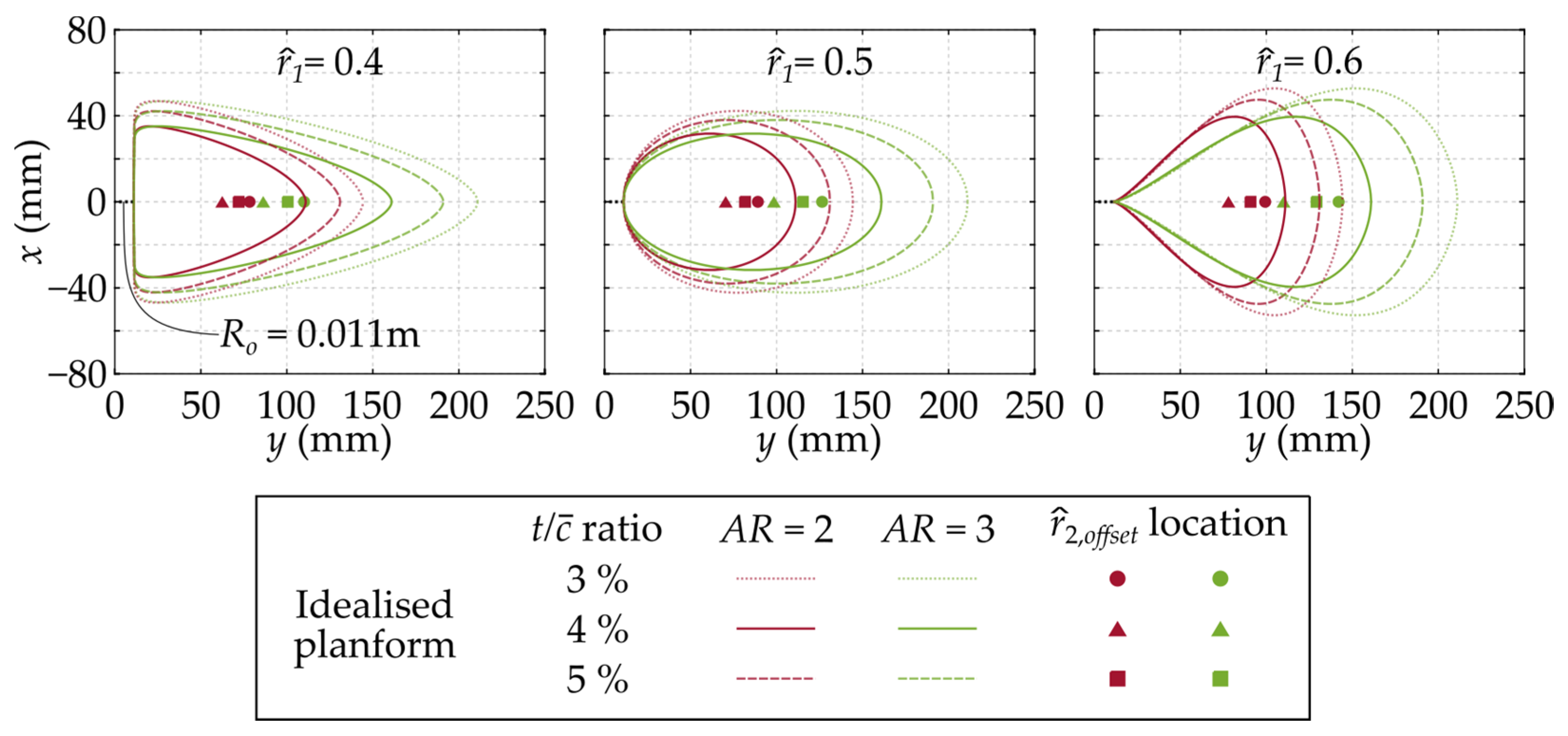
Figure 3.
Example angular displacement profiles of the fastest and slowest wings, at = 10,000. Different motion phases for each wing are demonstrated by arrows. Solid lines show what has been inputted to the motor and dotted lines show what has been measured with an external rotary encoder to check satisfactory operation of the servo motor.

Figure 4.
Example force histories for wing models = 2, = 0.4 and = 3, = 0.6 ( = 5%, = 10,000). (a) Drag coefficients are shown for both wing models as a function of rotational angle. (b) Lift coefficient histories as a function of chord lengths travelled at the second moment of wing area. (c) Drag coefficient histories shown instead as a function of chord lengths travelled at the second moment of wing area. Average chord length for both wing models was 60 mm.
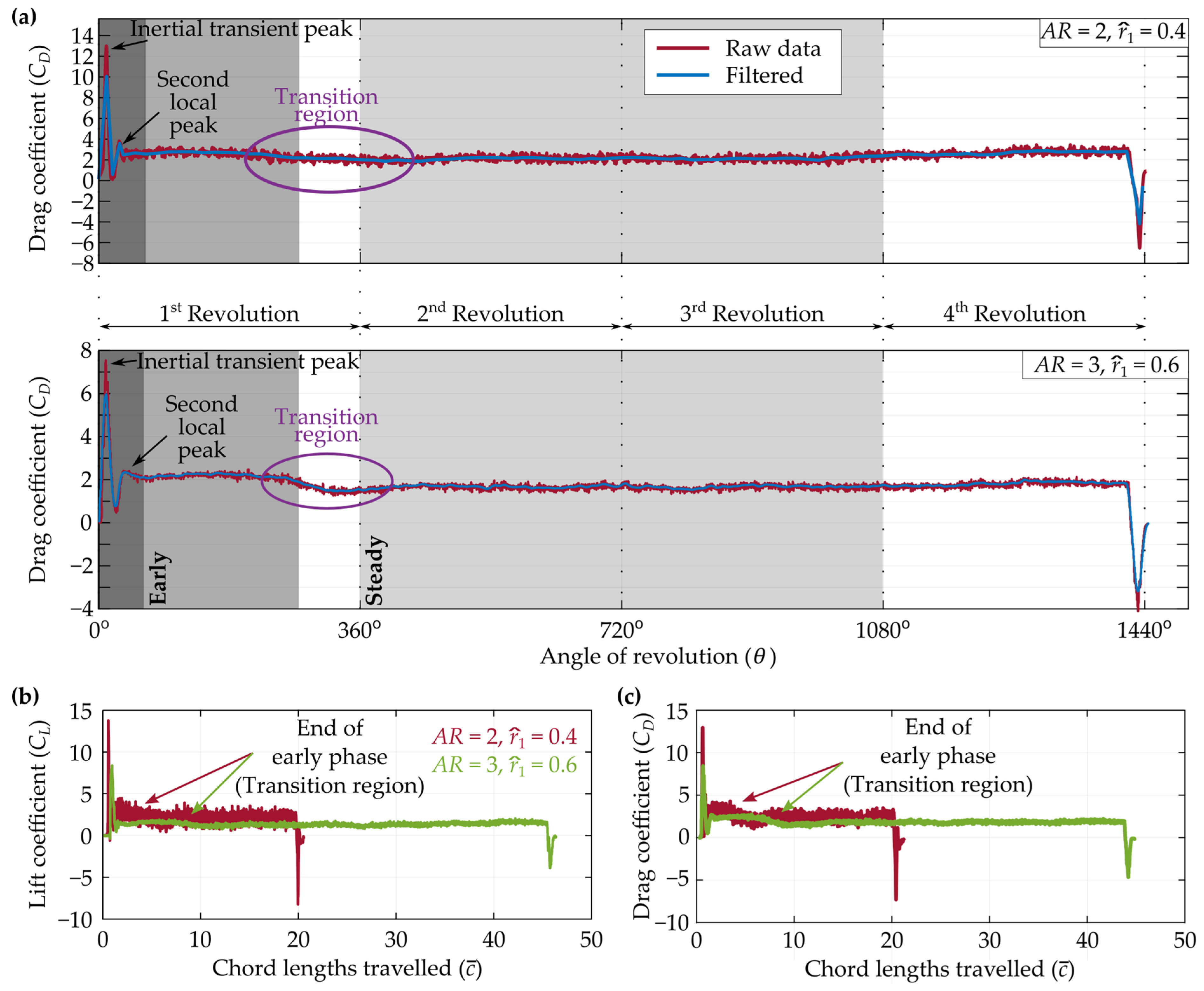
Figure 5.
Illustration of the techniques used to estimate the aerodynamic characteristics for an example wing configuration ( = 3, = 0.5, = 5%, =10,000). (a) Lift curve, and (b) drag curve. (C.I. denotes confidence interval).
Figure 5.
Illustration of the techniques used to estimate the aerodynamic characteristics for an example wing configuration ( = 3, = 0.5, = 5%, =10,000). (a) Lift curve, and (b) drag curve. (C.I. denotes confidence interval).

Figure 6.
Planform morphology effect on aerodynamic characteristics. This demonstration is for a thickness-to-chord ratio of 5% and Reynolds number of 10,000. (Top row) Lift coefficient vs. angle of attack. (Bottom row) Drag coefficient vs. angle of attack.
Figure 6.
Planform morphology effect on aerodynamic characteristics. This demonstration is for a thickness-to-chord ratio of 5% and Reynolds number of 10,000. (Top row) Lift coefficient vs. angle of attack. (Bottom row) Drag coefficient vs. angle of attack.
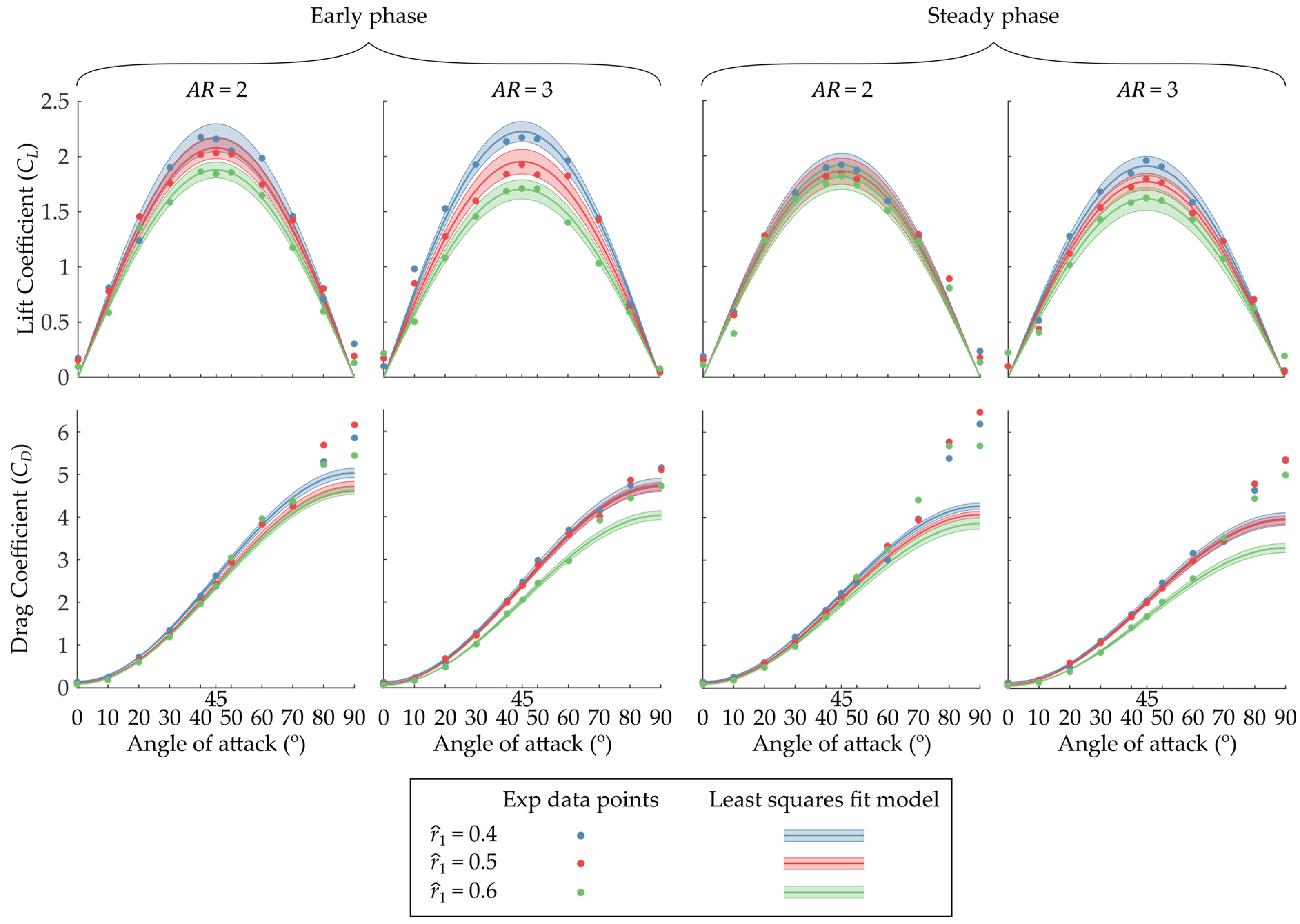
Figure 7.
Stacked bar chart showing the variation of (a) from early measurements, (b) from steady measurements, and (c) with area centroid location, , aspect ratio, , and Reynolds number, .
Figure 7.
Stacked bar chart showing the variation of (a) from early measurements, (b) from steady measurements, and (c) with area centroid location, , aspect ratio, , and Reynolds number, .
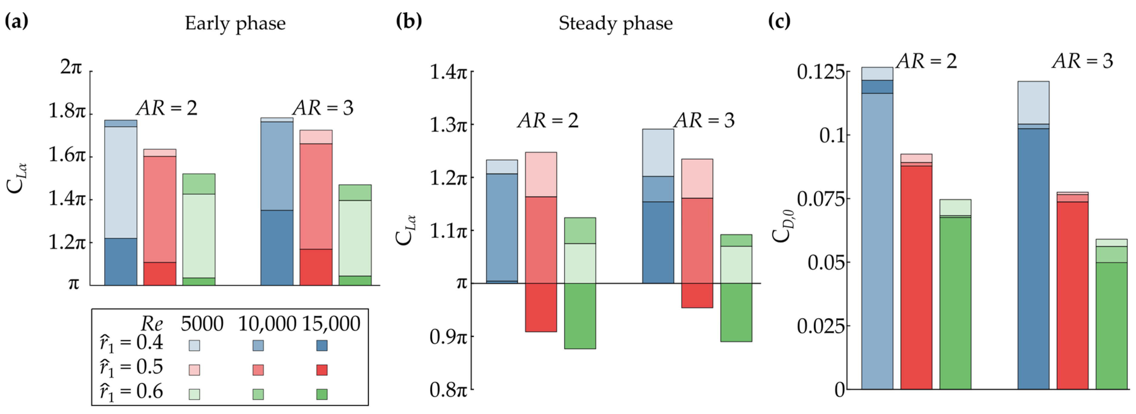
Figure 8.
Stacked bar chart showing the variation of (a) from early measurements, (b) from steady measurements, and (c) with area centroid location, , aspect ratio, , and thickness-to-chord ratio, .
Figure 8.
Stacked bar chart showing the variation of (a) from early measurements, (b) from steady measurements, and (c) with area centroid location, , aspect ratio, , and thickness-to-chord ratio, .
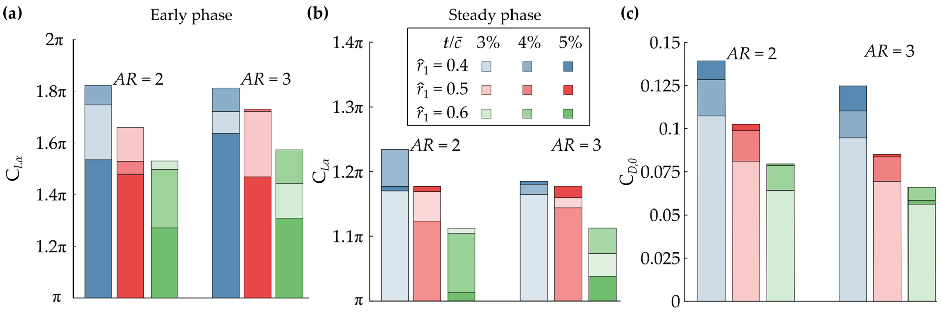
Figure 9.
Relation between lift and drag characteristics within the normal force model. Measurement points are shown via the asterisk markers. Blue and red lines demonstrate the slope of the best fit linear relation for the measurements, whereas the black lines show the locus where perfect equivalence should have been achieved.
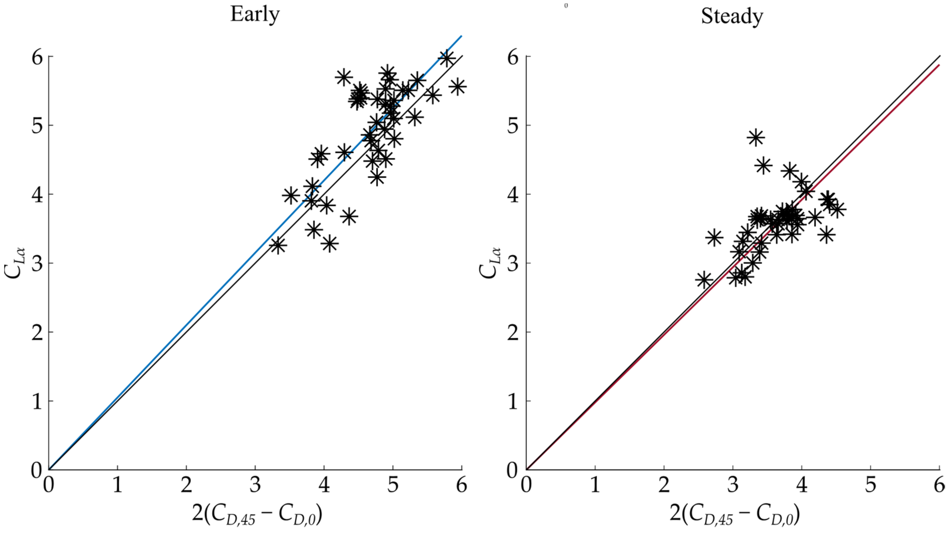
Figure 10.
Glide ratio vs. angle of attack. Lines are plotted based on the glide ratio definition provided by Equation (11) based on extracted lift curve slope and zero-lift drag coefficient values. The grey region represents the typical angle of attack operating region for insect flight. In (a), all thickness-to-chord ratio and Reynolds number cases were averaged for each centroid location value at each aspect ratio; in (b), all thickness-to-chord ratio and aspect ratio cases were averaged for each centroid location value at each Reynolds number; and in (c), all Reynolds number and aspect ratio cases were averaged for each centroid location value at each thickness-to-chord ratio.


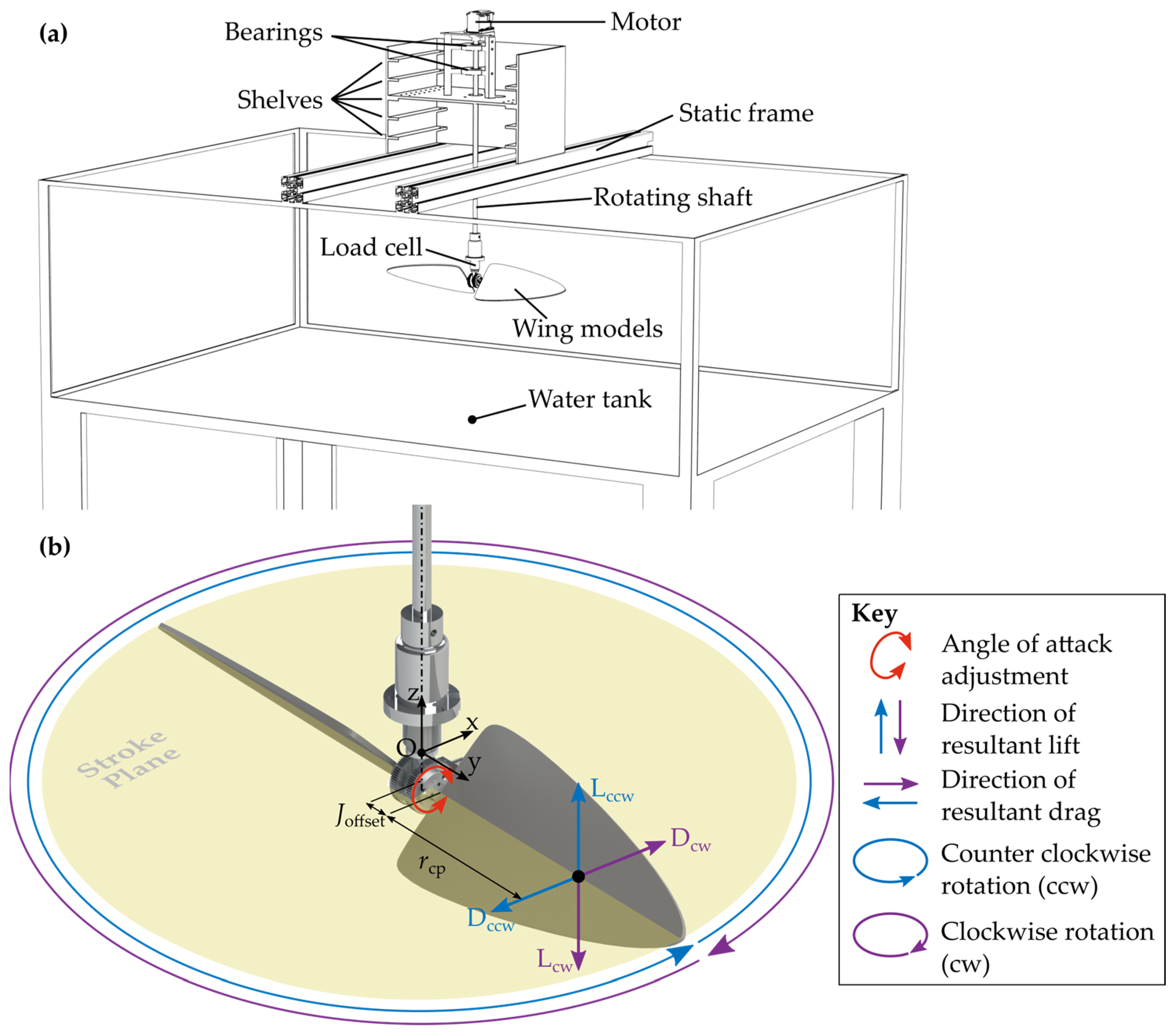
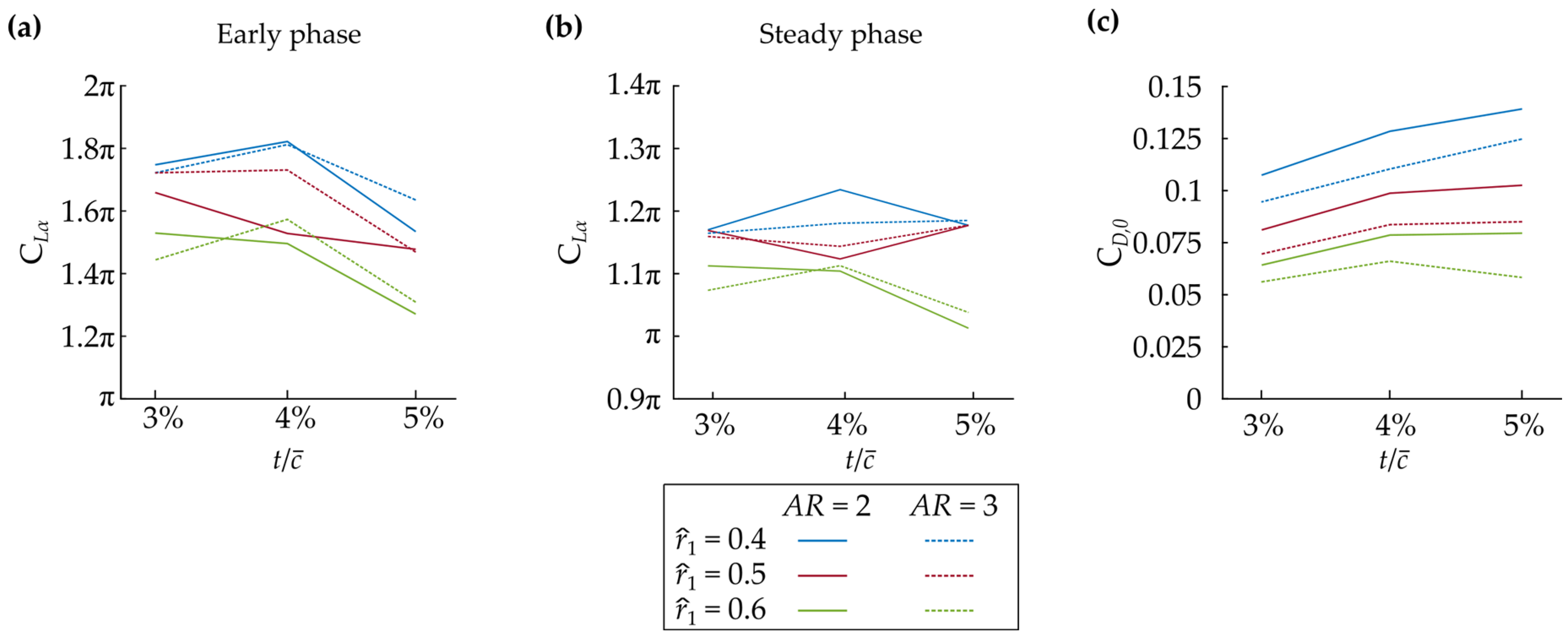
Table 1.
Manufactured wing models with main morphological variables and materials considered. * Variables defined by other parameters.
Table 1.
Manufactured wing models with main morphological variables and materials considered. * Variables defined by other parameters.
| Material | (mm) | (mm) | (mm) | |||||||
|---|---|---|---|---|---|---|---|---|---|---|
| Laser-cut acrylic | 5 | 3 | 60 | 2 | 120 | 0.092 | 0.4 | 0.476 | 0.509 | 0.554 |
| 0.5 | 0.559 | 0.589 | 0.626 | |||||||
| 0.6 | 0.639 | 0.665 | 0.691 | |||||||
| 3 | 180 | 0.061 | 0.4 | 0.476 | 0.498 | 0.546 | ||||
| 0.5 | 0.559 | 0.579 | 0.618 | |||||||
| 0.6 | 0.639 | 0.656 | 0.684 | |||||||
| 3D Printed PLA | 4 | 2 | 50 | 2 | 100 | 0.110 | 0.4 | 0.476 | 0.515 | 0.559 |
| 0.5 | 0.559 | 0.594 | 0.630 | |||||||
| 0.6 | 0.639 | 0.670 | 0.695 | |||||||
| 3 | 150 | 0.073 | 0.4 | 0.476 | 0.502 | 0.550 | ||||
| 0.5 | 0.559 | 0.583 | 0.621 | |||||||
| 0.6 | 0.639 | 0.660 | 0.687 | |||||||
| Laser-cut stainless steel | 3 | 2 | 66.7 | 2 | 133 | 0.083 | 0.4 | 0.476 | 0.505 | 0.552 |
| 0.5 | 0.559 | 0.586 | 0.624 | |||||||
| 0.6 | 0.639 | 0.663 | 0.689 | |||||||
| 3 | 200 | 0.055 | 0.4 | 0.476 | 0.495 | 0.545 | ||||
| 0.5 | 0.559 | 0.577 | 0.617 | |||||||
| 0.6 | 0.639 | 0.655 | 0.682 |
Disclaimer/Publisher’s Note: The statements, opinions and data contained in all publications are solely those of the individual author(s) and contributor(s) and not of MDPI and/or the editor(s). MDPI and/or the editor(s) disclaim responsibility for any injury to people or property resulting from any ideas, methods, instructions or products referred to in the content. |
© 2023 by the authors. Licensee MDPI, Basel, Switzerland. This article is an open access article distributed under the terms and conditions of the Creative Commons Attribution (CC BY) license (https://creativecommons.org/licenses/by/4.0/).
Share and Cite
MDPI and ACS Style
Broadley, P.; Nabawy, M.R.A. On the Validity of the Normal Force Model for Steadily Revolving Wings: An Experimental Investigation. Aerospace 2023, 10, 388. https://doi.org/10.3390/aerospace10050388
AMA Style
Broadley P, Nabawy MRA. On the Validity of the Normal Force Model for Steadily Revolving Wings: An Experimental Investigation. Aerospace. 2023; 10(5):388. https://doi.org/10.3390/aerospace10050388
Chicago/Turabian StyleBroadley, Paul, and Mostafa R. A. Nabawy. 2023. "On the Validity of the Normal Force Model for Steadily Revolving Wings: An Experimental Investigation" Aerospace 10, no. 5: 388. https://doi.org/10.3390/aerospace10050388
Note that from the first issue of 2016, this journal uses article numbers instead of page numbers. See further details here.