
UAV Path Planning Based on Improved Artificial Potential Field Method

School of Electrical and Electronic Engineering, Wuhan Polytechnic University, Wuhan 430048, China
*
Author to whom correspondence should be addressed.
Aerospace 2023, 10(6), 562; https://doi.org/10.3390/aerospace10060562
Submission received: 4 May 2023
/
Revised: 12 June 2023
/
Accepted: 12 June 2023
/
Published: 15 June 2023
(This article belongs to the Section Aeronautics)
Abstract
:The obstacle avoidance system of a drone affects the quality of its flight path. The artificial potential field method can react quickly when facing obstacles; however, the traditional artificial potential field method lacks consideration of the position information between drones and obstacles during flight, issues including local minima, unreachable targets, and unreasonable obstacle avoidance techniques that lengthen flight times and consume more energy get encountered. Therefore, an improved artificial potential field method is proposed. First, a collision risk assessment mechanism was introduced to avoid unreasonable obstacle avoidance actions and reduce the length of unmanned aerial vehicle flight paths. Then, to solve the problem of local minimum values and unreachable targets, a virtual sub-target was set up and the traditional artificial potential field model was modified to enable the drone to avoid obstacles and reach the target point. At the same time, a virtual sub-target evaluation factor was set up to determine the reasonable virtual sub-target, to achieve a reasonable obstacle avoidance path compared to the traditional artificial potential field method. The proposed algorithm can plan a reasonable path, reduce energy consumption during flight, reduce drone turning angle changes in the path, make the path smoother, and can also be applied in complex environments.
1. Introduction
Unmanned aerial vehicle use has been expanding quickly in recent years [1]. They are extensively utilized in a variety of contexts, including military reconnaissance, rescue operations, and environmental preservation [2]. Path planning is one of the main technologies for ensuring a drone’s smooth flight and safe and successful obstacle avoidance [3]. A* algorithm [4], genetic algorithm [5], particle swarm optimization [6], ant colony optimization [7], RRT algorithm [8], velocity obstacle [9,10], reinforcement learning method [11,12,13], artificial potential field method [14,15,16,17,18,19,20,21,22], and others are examples of commonly used path planning methods.
Due to its advantages such as low computation, real-time capability, easy control, and good robustness relative to other algorithms [23], the artificial potential field method stands out among many algorithms. However, traditional artificial potential field methods may suffer from problems such as local optima, unreachable goals, and unreasonable planned paths due to their limitations. Many scholars have conducted research to address the above issues. Feng et al. [15] redefined the repulsive impact range by adding a safety distance to the potential field model based on real environmental conditions, and divided the threat level of obstacles, taking into account the constraints on the vehicle’s speed in the repulsion calculation. Yang et al. [16] solved the problem of unreachable goals by modifying the attractive model to increase the robot’s attraction to the target point; they also set virtual target points and evaluations to avoid local minimum points. However, virtual sub-targets have not been set by considering the relative positioning information between the robot and obstacles. Feng et al. [17] set a virtual obstacle at the local minimum point of the drone. The virtual barrier provides repulsive force to the drone, causing it to escape from the local minimum area in the past tense, when facing dynamic obstacles avoidance, there will be a sudden change in the drone’s angle, which affects the drone’s flying performance. Azzabi et al. [18] added the minimum distance between obstacles and target points to the traditional attractive potential field function, increasing the attraction near the target point to solve the problem of unreachable targets while also reducing the computation time. By setting an escape force, when a drone falls into a local minimum, the escape force is activated to prompt the UAV to leave the local minimum point. The lack of consideration for smooth handling at the joint connections has resulted in excessively large angles at the turning points. In the case of encountering a local minimum, Fedele et al. [19] used rotating force to enable the robot to bypass obstacles. They also designed a potential field-switching mechanism when faced with multiple obstacles to smooth out continuous obstacle avoidance paths. To tackle the issue of unreachable targets, Fan et al. [20] incorporated the Euclidean distance between the robot and the target point into the repulsive potential field function. The robot can reach the target by generating a force pointing toward the target point. In dealing with local minimum problems, they created virtual hexagons for the robot to follow as it escapes from virtual sub-target points. The robot did not take into account the distribution of subsequent obstacles when traversing the virtual hexagon, resulting in path planning that is too long. During the process of obstacle avoidance in unmanned aerial vehicles (UAVs), it is necessary to calculate the collision risks of obstacles in the external environment. The velocity obstacle method utilizes the relative velocity between objects to calculate the collision area [9]. In addition, Jenie et al. [10], in situations when there is a lack of communication between UAVs and obstacles, optimization of obstacle avoidance methods is achieved through the introduction of perception and evasion, making it possible for UAVs to avoid obstacles in non-cooperative situations.
Regarding the problem of flight path length, Jiang et al. [21] proposed adaptive step size adjustment to reduce the length of the obstacle-avoidance path in the traditional artificial potential field method. Li et al. [22] incorporated the ratio of the total length of the path to the current distance from the target into the path calculation to obtain an adaptive step size. Both approaches were aimed at reducing the length of the obstacle-avoidance path.
In the context of known information about the position and size of static obstacles, this paper aimed to design an artificial potential field drone obstacle avoidance scheme based on collision risk strategy. The contribution of this study includes the following aspects: Firstly, introducing a collision risk judgment mechanism based on a safe distance. The drone determines whether there is a collision risk based on its current position and flight direction, and the obstacle’s location, thereby improving the drone’s impact judgment on obstacles, eliminating the repulsion generated by non-obstructing obstacles, avoiding unnecessary obstacle avoidance actions, and reducing energy consumption. Secondly, setting up virtual sub-goals and evaluation factors. Virtual sub-goals generate control forces to make drones avoid obstacles and reach safe areas. By setting evaluation factors for virtual sub-goals, the reasonable virtual sub-goal can be selected for reasonable flight paths. Introducing an adaptive step size setting, the drone adjusts the step size in different areas to reduce the flight path length with flight times.
The organization structure of this article was as follows: Section 2 introduced the basic principles of traditional artificial potential field methods and the problems encountered. Section 3 provided a detailed description of the improved artificial potential field method. Section 4 conducted simulation experiments and discussions. Section 5 discussed the improved algorithm. Section 6 summarized this article and presented outlooks for the future.
2. Traditional Artificial Potential Field Method
The basic concept behind the traditional artificial potential field approach is to use a virtual potential field to describe the position information between the UAV and the target location and between the UAV and the obstacle [24]. According to the distance connection in the potential virtual field, the target point attracted the UAV while the barriers repel it to the extent of their impact. Until it reaches the target spot, the UAV maneuvers by force which results in attraction and repulsion. The following Formula (1) represents the combined potential field of the conventional artificial potential field approach.
According to the formula, Uatt(goal) the target location generates a field of gravitational attraction toward the drone, and Urep(obs) is the barrier that generates the repulsive potential field. The letter “m” denotes the number of barriers.
In Formulas (2) and (3), the gravitational potential field Uatt(goal) and the repulsive potential field Urep(obs) functions, respectively, are shown.
This formula uses constants katt and keeps to represent the attractive potential gain coefficient and repulsive potential gain coefficient, respectively. It also uses Pu to represent the drone’s position, Pgoal to represent the target point’s position, ρ(Pu, Pgoal) to represent the Euclidean distance between the two, Pobs to represent the obstacle’s position, ρ(Pu, Pobs) to represent the Euclidean distance between the two, and ρeff to represent the obstacle’s influence distance. As stated in Equations (4) and (5), the attractive force Fatt(goal) and the repulsive force Frep(obs) can be calculated by calculating the negative gradient of the potential field function.
where is the unit vector where the drone points to the target point, is the unit vector where the obstacle points to the drone.
Equation (6) can be used by the drone to calculate the total force of Fall that it is currently experiencing during flight by adding the attractive force from the point of the goal and the repulsive force generated by the obstacles.
A particular distance threshold is used to calculate repulsion in the traditional artificial potential field method for path planning, which results in an abrupt change in repulsion. However, attraction persists along the entire planned route. In light of this, the traditional artificial potential field approach has the following problems:
- (1)
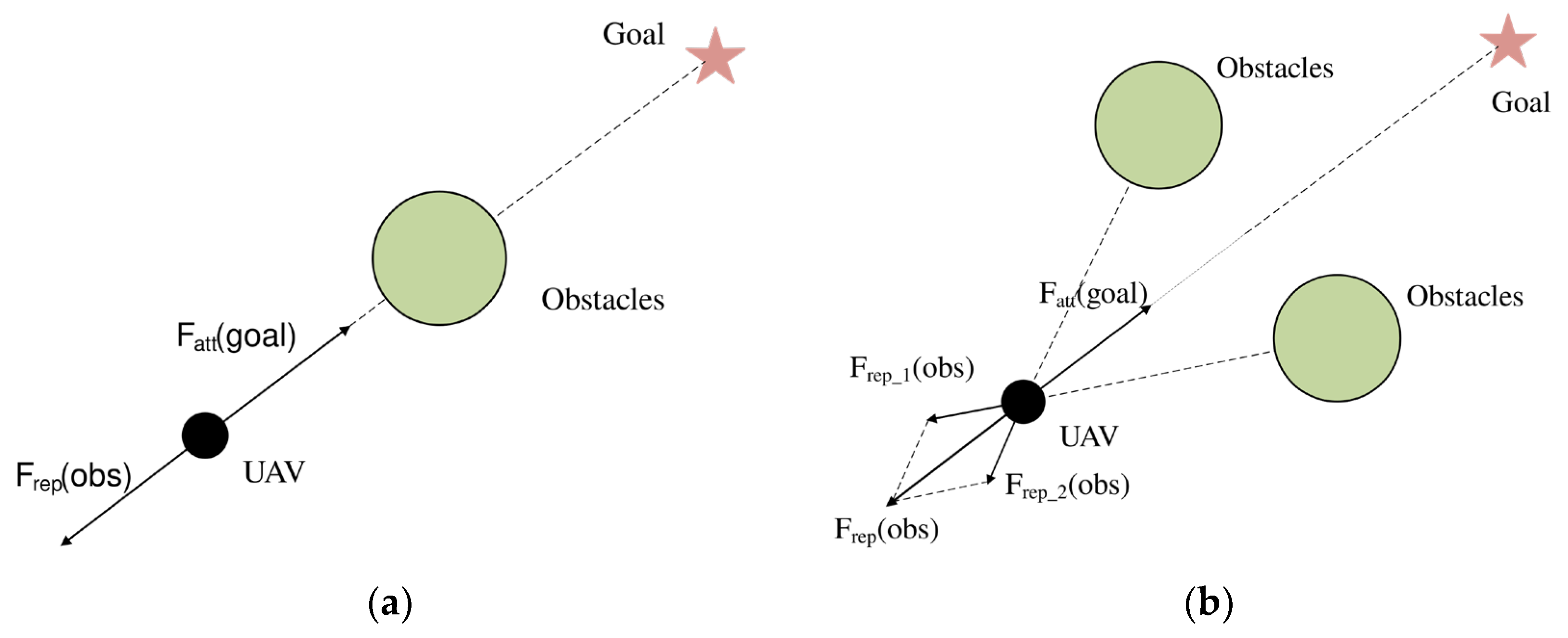
- The local minimum value problem [25]. Figure 1a illustrates what happens when the drone, obstacle, and target point are all situated in a straight line: the drone will be in a state of force balance, unable to progress to the next position, and unable to reach the target point. As seen in Figure 1b, the drone encounters equal and opposing repulsive and attractive forces from the obstacles at a given point, forcing it to stall at this location.
- (2)
- (3)
- Unreasonable motions are made to avoid obstacles. Even though the position of obstacles in front of the drone has no bearing on its forward path, as illustrated in Figure 3, when the forward path reaches within the obstacle’s influence range, the drone will produce obstacle avoidance movements, lengthening the path.
This article introduces a collision risk judgment method based on a safe distance that reduces the drone’s irrational motions while in flight. A virtual sub-target is introduced and an evaluation is set for the virtual sub-target to deal with the problems of local minimum values and unreachable goals. To get the drone to the target position, a method for setting virtual sub-targets is developed. At the same time, sudden repulsion forces are removed from the traditional artificial potential field models. Adaptable step size is suggested following various threat regions to reduce the drone’s flight time.
3. Improvement of Artificial Potential Field Method
In the case of known static obstacle information, to address the above issues, this section improves upon the artificial potential field method. Based on the speed obstacle method for collision evaluation between objects, a collision risk judgment mechanism based on a safety distance angle is proposed. To address situations where drones have collision risks during flight or are stuck in a local minimum value, virtual sub-targets are proposed to guide drones to avoid obstacles and escape local minimum value points. Since the quality of the virtual sub-target setting also affects the quality of the drone’s flight path, a virtual sub-target evaluation factor is introduced based on the virtual sub-target, target point, and obstacle information between the virtual sub-target and the target point to obtain a reasonable virtual sub-target. The traditional artificial potential field method model is modified based on the collision relationship and virtual sub-target. Finally, an adaptive step size setting is proposed based on the geometric relationship between the drone and obstacles to improve the drone’s flight performance. At the same time, the obstacle model in this paper is set as circular. When facing non-circular obstacles, the obstacle model is built by constructing the circumscribed circle.
3.1. The Mechanism for Calculating Crash Risk Based on Safety Distance
Obstacle avoidance is essential for drones to fly safely and steadily in their environment. As Equation (5) demonstrates, the geometry relationship between the drone and the obstacle is not considered by the traditional artificial potential field method, which only considers the distance between the drone and the obstruction to calculate the obstacle’s repulsive force on the drone. As seen in Figure 4, when there are no angle constraints, meaning that the relationship between the current heading angle of the unmanned aerial vehicle (UAV) and the obstacle is not judged [10] and the UAV will not be affected by obstacles in front of it during its path, but if the planned path falls within the influence range of an obstacle, the obstacle will still exert a repulsive force on the UAV, causing the UAV to increase its avoidance movements, resulting in higher energy consumption [26] and path length.
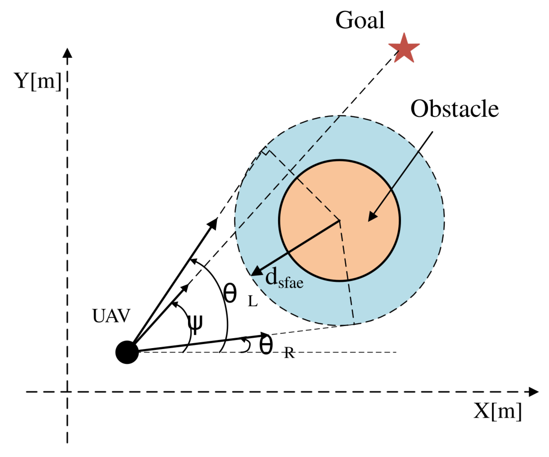
To address this problem, a mechanism for judging the likelihood of a collision based on the safety distance angle was developed [15]. Based on the speed obstacle method for evaluating collision risks between unmanned aerial vehicles and obstacles [10], this article incorporated the heading relationship between the UAV and obstacles into the collision risk calculation. At the same time, a safety distance was introduced within the obstacle model to increase the buffer zone between the UAV and the obstacles. At the same time, a safety distance dsafe was added to the obstacle model, as illustrated in Figure 5, to predict the collision between drones and obstacles [27]. As a buffer zone between the drone and the obstacle, the safety distance dsafe added to the radius of the drone outside of the obstacle.
In Formula (7), the safety distance dsafe is defined as follows:
where the UAV radius is do and du is the obstacle radius. Using Formula (8), the angle ψ of the drone’s current flight path is compared to the angle (θR, θL) of the obstacle’s boundary to assess the probability of collision:
As demonstrated in Figure 6, there is a risk of collision when the present angle of UAV A is on the edge of an obstacle with a safety distance. The UAV must avoid the impediment in this situation, which will be covered in a subsequent section. There is no risk of a collision when the UAV’s present angle is outside the obstacle’s perimeter with a safety distance, and thus it can continue to fly in its current direction.
3.2. Virtual Sub-Target Setting
During the flight process, the drone encountered the following situations:
Situation 1: when there is the possibility of a collision due to the drone’s trajectory forward;
Situation 2: when the drone is in a local minimum [25].
When the drone is in the above Situation 1, it may have collision risk under the action of potential field force and needs to avoid obstacles during flight. The traditional artificial potential field method may cause sudden changes in the drone’s turning angle during obstacle avoidance due to the sudden increase of repulsive force, affecting the flight performance of the drone.
When the drone is in Situation 2, it is trapped in a point and unable to reach the target due to the balance of potential field force and needs to escape from this local minimum trap. To solve the problems of excessive turning angle caused by collision risk with obstacles and stopping or hovering due to local minimum traps during flight, due to the limitations of the drone’s flight turning performance during actual obstacle avoidance flight, it cannot achieve large angle changes in reality [28,29]. This article introduces a virtual sub-target to enable the drone to avoid obstacles or escape from local minima while reducing the angle changes in the flight path to meet the requirements of practical flights.
As shown in Figure 7, the current UAV position Pcur_uav(xu, yu) is the origin, and the detected distance dpre is the radius to detect the obstacle within the angle β in front of the UAV. When the detection of obstacles ahead Pr_col(xobs, yobs) has the risk of collision or in the case of local minima, a virtual sub-target is generated to guide the UAV to the target point. The specific method is to make the UAV and the obstacle line L1 of the vertical line L2, L2, and the safe distance dsafe intersect with two points for Pdum_i (i = 1, 2); that is, the virtual sub-target coordinates to be determined. The slope of the UAV obstacle line L1 is k1, and the coordinates of the virtual sub-target Pdum_i(xdum_i, ydum_i) (i = 1, 2) are given by Equations (9) and (10).
3.3. Virtual Sub-Target Evaluation
The influence of obstacle distribution on the drone’s path has received less attention in the existing research than the setting of virtual waypoints based on the dimension of the drone’s heading deviation angle [30,31], obstacles near local minima [17,25,32], and information on obstacle distribution [33].
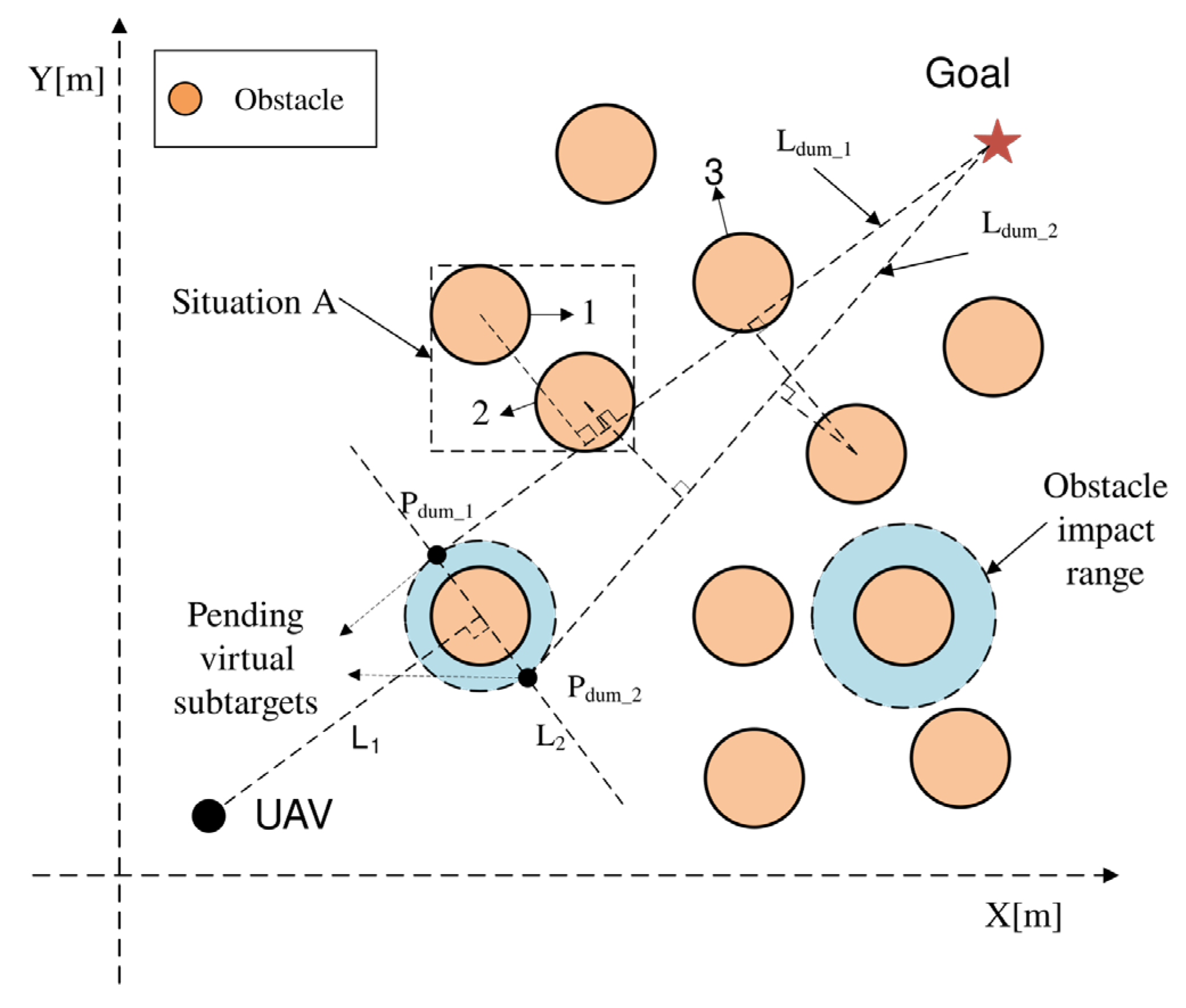
The virtual sub-target setting had an impact on the subsequent path of the drone; therefore, this paper proposed a virtual sub-target evaluation factor to reasonably estimate the flight path of the drone and reduce drone energy consumption. As shown in Figure 8, the virtual sub-target Pdum_i (i = 1, 2) was set and connected with the target point by line Ldum_i (i = 1, 2), and the distances from the obstacles in front of line L2 to line Ldum_i (i = 1, 2) were represented as ρ(Pobs_j, Ldum_i). When the line Ldum_i fell within the influence range of obstacles 1 and 3, the drone needed to generate obstacle avoidance actions to avoid them. At the same time, considering the effect of scenario a formed by obstacles 1 and 2 on the line, the obstacles within the range of 4ρeff from line Ldum_i were included in the evaluation calculation. All these descriptions are in the past tense because it is explaining what has already been proposed and done in the article.
Equation (11), for example, states that the relative distance between the obstruction and the line Ldum_i (i = 1, 2) is defined as ω. The relative distance ω is determined to determine how impediments (such as obstacles 1 and 3) affect the line Ldum_i. After that, the effectiveness of establishing virtual sub-goals is assessed using the assessment factor J. Equation (12) is the expression for the evaluation factor J.
In the equation, m represents the number of obstacles whose distance from the line Ldum_i, as represented by distance ρ(Pobs_j, Ldum_i), is greater than 4ρeff (ρ + α) is the evaluation distance and α is the evaluation constant.
When ω < 0, it meant that the drone needed to avoid the obstacle because it was close to the line Ldum_i evaluation distance. When ω ≥ 0, it meant that the obstacle was outside of the line Ldum_i evaluation range and that the drone did not need to avoid it. Based on the value of ω, the value of J might is i determined. When a particular virtual sub-goal assessment factor J is smaller, it means that the obstacles close to the line Ldum have less of an effect on the drone’s future flight route; thus, a reasonable virtual sub-target coordinate can be derived Pdum(xdum, ydum).
3.4. Artificial Potential Field Model Modification
The virtual sub-goal Pdum(xdum, ydum) has no obstacles between its location and the current position of the drone. Therefore, it is possible to eliminate the repulsive force generated by obstacles in traditional artificial potential field methods and only retain the attraction generated by the target point. The attraction in traditional artificial potential field methods is only based on the distance between the drone and the target point. As the drone gets closer to the target point, the value of the attraction also decreases, which can make it difficult for the drone to accurately reach the target point.
The target attraction calculation in traditional artificial potential field methods was improved in this article concerning the aforementioned problem by taking into consideration the ratio of the distances ρ(Ps, Pgoal) between the drone’s starting point and the target point and ρ(Pcur_uav, Pgoal) between the drone’s current position and the target point. The enhanced attraction force Fimp_att(goal) can offer more attraction as the drone gets closer to the target point, enabling it to be reached precisely. Equation (13) provides the expression for the enhanced attraction force Fimp_att(goal).
The parameter λ satisfies Equation (14):
When the virtual sub-target was present, the gravitational pull was generated by both the target point and the virtual sub-target, as well as regulatory gravitational force. The drone moved to the following location thanks to a combination of gravitational attraction at the target point and the regulating gravitational force of the virtual sub-target. The equation for the regulatory gravitational force Fimp_att(goal) of the virtual sub-target is given by Equation (15). It is derived depending on the distance ρ(Pcur, Pdum) between the drone and the virtual sub-target.
is the distance parameter in the equation.
Equation (16) provides the expression for the total attractive force Fatt on the drone following Equations (13) and (15).
3.5. Adaptive Step Size
The step size of an unmanned drone vehicle flight determined the distance of each step, thereby affecting the flight time and energy consumption during the flight process. An adaptive step size setting has been suggested to lessen the number of drone flights to increase UAV flight efficiency [34]. When there is no collision risk ahead of the drone, the step size should be raised within the detection distance dpre to accomplish fast flight. The step size should be decreased to avoid obstacles when there is a chance of collision in front of the drone.
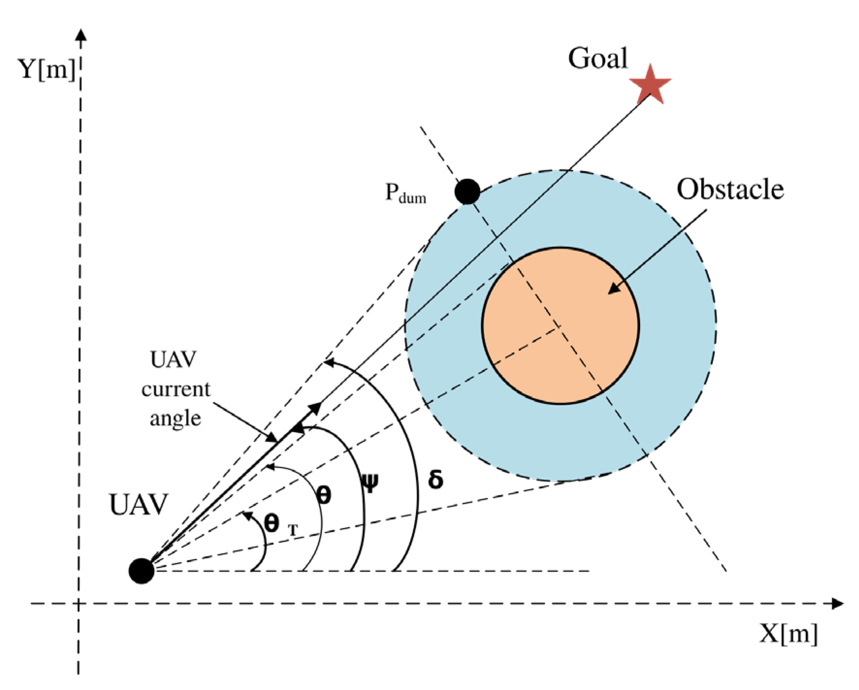
As shown in Figure 9, determine the drone’s subsequent step length based on the current angle ψ, the obstacle boundary angle θ, the angle between the drone and the obstacle connecting line θT, the fixed step size St, the virtual sub-target boundary angle , and the current angle L. Equation (17) gives L the step length expression.
Equation (17), (δ − θ) represents the escape angle, and (θ − θT) represents the collision angle.
If the drone’s angle ψ is greater than the obstacle’s boundary angle θ, the drone’s angle to the escape angle is increased. Considering the angle relationships between the drone, the virtual sub-target, and the obstacles. The value of Equation (17(a)) gradually rises as the angle of the drone increases since the likelihood of a collision diminishes. The ratio of the drone’s angle to the collision angle is added if the angle of the drone ψ is shorter than the angle of the obstacle’s boundary θ. The value of Equation (17(b)) steadily reduces when the drone’s angle drops because there is a greater chance of a collision.
Although the step size computation is shown in Equation (17), both excessively large and excessively small step sizes still affect the drone’s flying, necessitating a limit on the step size. The step size’s final expression is given in Equation (18), and this paper determines an upper limit for the step size lmax = 1.8St and a lower limit for the step size lmin = 0.8St:
4. Comparison of Simulation Results
The traditional artificial potential field method (referred to as T-APF) and the algorithm in reference [30] (referred to as B-APF) were tested and simulated under the conditions of local minimum value, unreachable target, and complex environment to confirm the viability and effectiveness of the algorithm proposed in this paper (referred to as IM-APF). Table 1 and Table 2 display the parameters of the method; the autonomous drone’s flying height and the wind speed in the flight environment were both fixed at the same time.
To evaluate the flight performance of drones under three algorithms, this article compared the length of the path (Jlength), energy consumption (E) during flight, number of iterations (N), angle changes, and number of angle changes in the drone flight path.
Equation (19) provides the formula to calculate the UAV’s entire flight path length [35], abbreviated as Jlength:
where I is the total number of steps in a drone flight.
Based on the UAV’s horizontal speed and acceleration, it is possible to determine the energy consumption P of the battery during flight [36]. Equation (20) can be used to determine the general consumption of energy E during flight:
where T is the amount of time the drone spent flying overall.
4.1. Local Minimal Value Test Verification
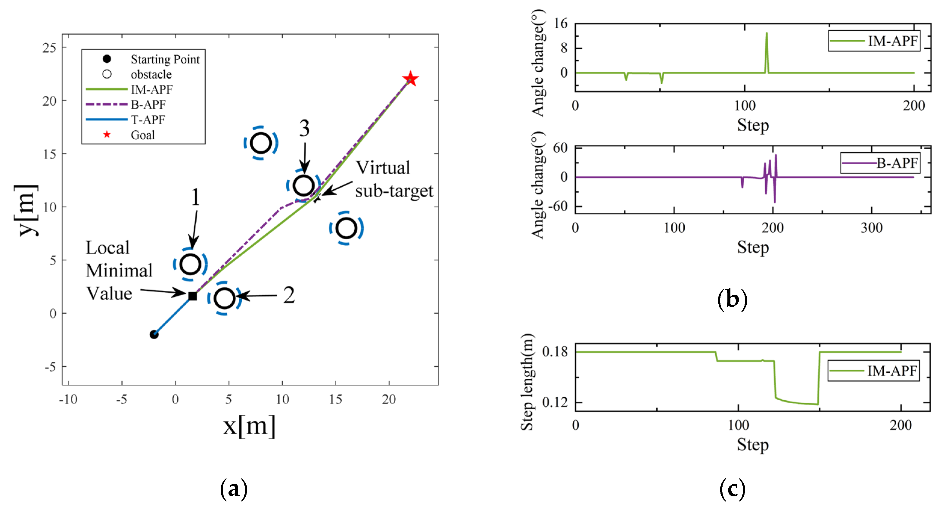
Three simulation scenarios were set up in this study to test the algorithm’s efficacy in dealing with local minima, as depicted in Figure 10a, Figure 11a and Figure 12a. Local minimum case 1 in Figure 10a is established by aligning obstacles 1 and 2 symmetrically about the line linking the UAV and the target point, whereas local minimum case 2 is established by placing obstacle 3 on the line that connects the UAV start point and the target point. In Figure 11a, the target point stands between obstacles 1 and 3, forming local minimum case 3, which is on the line that connects the UAV start point with the target point. In Figure 12a, obstacles 1 and 3 are present on the line that connects the UAV start point and the target point, forming local minimum case 4.
Due to force balancing, the UAV will stop in front of obstacles when the T-APF algorithm runs into the aforementioned four local minima and will be unable to reach the target point. The IM-APF and B-APF algorithms, on the other hand, can bypass the local minimum and arrive at the desired location. The IM-APF algorithm generates a virtual sub-target outside the safety distance of the obstacles when it encounters local minima, and it chooses an appropriate evaluation factor for the virtual sub-target. In addition to helping the UAV escape the local minimum trap, the virtual sub-target also lessens the UAV’s activities to avoid obstacles as it approaches the virtual sub-target.
Figure 10b, Figure 11b and Figure 12b show the drone angle change diagrams for the IM-APF and B-APF algorithms in the three scenarios. The IM-APF algorithm’s greatest angle change during obstacle avoidance in all three scenarios was roughly 36.30°. In Scenario 2, the B-APF algorithm encountered obstacle 2 and in Scenario 3 encountered obstacle 1, resulting in a significant angle change with the maximum angle change value reaching 96.34°. On the other hand, the IM-APF algorithm reduced the angle change by over 63.32% compared to the B-APF algorithm. Figure 10c, Figure 11c and Figure 12c depict the step change that occurs while the IM-APF algorithm is attempting to avoid obstacles. To shorten flight times, the drone flies at its maximum step length without the risk of collision. To counteract the drone’s fast speed and sluggish reaction time, the step length will be shortened when it comes into contact with objects that pose a risk of collision while in flight.
Table 3 displays the evaluation information for the three algorithms. In all three cases, the IM-APF and B-APF algorithms were able to avoid local minima. However, the IM-APF algorithm lengthened the drone’s flight route by 0.97% in comparison to the B-APF method. The IM-APF algorithm also decreased flight time and avoidance actions as a result of the virtual sub-target setup and evaluation factor, which led to a reduction in energy consumption during the flight by 33.64%. The IM-APF algorithm also improved by 44.01% in terms of the number of algorithm iterations.
4.2. Target Unreachable Test Validation
Three simulation scenarios were put up in this research to validate the algorithm’s efficacy in managing unreachable targets, as illustrated in Figure 13a, Figure 14a and Figure 15a. In each of the three simulation scenarios, the target spots are close to an obstruction. The drone will hover close to the target position when the T-APF algorithm hits an impassable target since it cannot be reached because the obstacle’s repulsive force is larger than its attraction force. On the other hand, the IM-APF and B-APF algorithms are unaffected by the repulsive force close to the target location and can reach it. At the same time, in Scenario 2, the drone successfully reached the target point despite facing obstacles 2, 3, 4 and 5, which formed a complex environment with an L-shaped obstacle. IM-APF algorithm, as opposed to the B-APF algorithm, chooses a sensible path in flight when confronted with complicated impediments because of the evaluation factor for virtual sub-target point selection.
Figure 13b, Figure 14b and Figure 15b display the drone angle change diagrams for the IM-APF and B-APF algorithms in the three scenarios. In all three scenarios, the IM-APF algorithm reduced the angle change and the number of steps for the drone to avoid obstacles compared to the B-APF algorithm. During obstacle avoidance, the IM-APF algorithm encountered a maximum angle change of 44.89° when facing obstacles in all three scenarios, while the B-APF algorithm had a maximum angle change of 58.69° in Scenario 1 when encountering obstacle 2, and experienced angle oscillations when encountering obstacles 4 and 5 in Scenario 2 and obstacles 1 and 2 in Scenario 3, with the maximum angle change reaching 88.32°. On the other hand, the T-APF algorithm had a maximum angle change of 320.79° in all three scenarios. The IM-APF algorithm reduced the angle change by over 49.17% compared to the B-APF algorithm. Reducing the angle change can lead to a decrease in energy consumption during the drone’s flight. Figure 13c, Figure 14c and Figure 15c illustrate the step change that occurs when the IM-APF algorithm is avoiding obstacles. In the absence of a risk of collision, the drone uses its maximum step length to cut down on flight duration. However, the step length is decreased to prevent flying too rapidly and causing collisions due to the drone’s delayed reaction when it comes into contact with objects that pose a risk of collision during flight.
The evaluation data for the three algorithms in the unreachable target scenario are shown in Table 4. Compared to the B-APF algorithm, the IM-APF algorithm increased the drone’s flight path length by 0.7988% in all three scenarios. Moreover, due to the shorter flight time and reduced angle change during the drone’s flight, the IM-APF algorithm reduced energy consumption by 34.78%. Finally, due to the presence of adaptive step length adjustment, the IM-APF algorithm reduced the number of iterations by 43.52%.
4.3. Complex Environment Test Verification
As shown in Figure 16a, Figure 17a and Figure 18a, three simulation scenarios were proposed in this study to verify the effectiveness of the algorithm in dealing with complex obstacle situations. To verify the effect of facing obstacles of different shapes, different-shaped obstacles (such as obstacles 1–7) were set in Figure 18a. Figure 16a illustrates how the T-APF algorithm encountered obstacles 2 and 4 in a complex environment, causing the drone to make an abrupt turn due to the repulsive force of the obstacles. As shown in Figure 17a, when encountering numerous obstacles, the T-APF algorithm made the drone unable to move at position A.
In a complex environment, both the IM-APF and B-APF algorithms were able to reach the target point. The B-APF algorithm selected a smaller angle by calculating the next turning angle of the drone to avoid obstacles. However, it did not consider the distribution of obstacle positions, which would increase the number of obstacle avoidance actions. Therefore, as shown in Figure 16a, when the drone avoided obstacle 2, it still needed to avoid obstacle 3, resulting in redundant obstacle avoidance actions. In Figure 18a, the drone still needed to avoid obstacles on the subsequent path after avoiding obstacle 1. The IM-APF algorithm selected a suitable virtual sub-target based on the distribution of obstacles between the obstacles and the target point. As shown in Figure 16a, the IM-APF algorithm only needed to avoid obstacle 2, reducing subsequent obstacle avoidance actions. At the same time, as shown in Figure 17a and Figure 18a, when facing complex environments and obstacles of different shapes, the IM-APF algorithm could choose a reasonable path and reach the target point simultaneously.
Figure 16b, Figure 17b and Figure 18b show the angle changes of the drone in three different scenarios. The maximum angle change of the IM-APF algorithm during obstacle avoidance in the three scenarios was 34°. The B-APF algorithm had a maximum angle change of 78.14° when facing obstacle 3 in Scenario 1, 87.71° in Situation 1 where there were two obstacles in Scenario 2 and 106.32° when facing obstacle 6 in Scenario 3. Compared with the B-APF algorithm, the IM-APF algorithm reduced the angle change by 68.02%, making the path smoother. As shown in Figure 16c, Figure 17c and Figure 18c, the IM-APF algorithm could still adjust the step size based on the collision risk with obstacles in a complex obstacle environment.
The evaluation data of the three algorithms in complex environments are shown in Table 5. When facing a complex environment, the IM-APF algorithm reduced the drone’s flight path length by 3.39% in the three scenarios compared to the B-APF algorithm. In addition, due to the virtual sub-target setting and evaluation factor of the IM-APF algorithm based on obstacle and drone flight path information, it selected a reasonable virtual sub-target, reducing unnecessary obstacle avoidance actions and unreasonable paths during the drone flight process, thus reducing energy consumption during flight. The energy consumption during the flight was reduced by 36.45%. Finally, in terms of algorithm iteration times, the IM-APF algorithm automatically adjusted the step size based on obstacle and flight information to reduce flight time when facing obstacles in complex environments. Therefore, the iteration times of the IM-APF algorithm were reduced by 62.82% compared to those of the B-APF algorithm.
5. Discussion
The artificial potential field method has been improved by some scholars to increase its practicality in various situations. The traditional method includes incorporating the Euclidean distance between the drone and the target point into the potential field function, as well as increasing the drone’s attraction to the target to solve the problem of hovering around the target. When the drone enters a local minimum trap in the flight environment, this article gives additional attraction by creating a virtual sub-target in the flight environment of the drone, as shown in Figure 10, Figure 11 and Figure 12, where B points are generated outside the obstacle for safety. When there is a risk of collision in the flight environment of the drone, the target point of the drone is increased with the virtual sub-target B point, which produces an attractive force on both. By calculating the distance between the drone and the virtual sub-target point as the calculation of the attractive force produced by the virtual sub-target, the drone can fly towards the virtual sub-target point. At the same time, because there is no obstacle threat between the virtual sub-target point and the current position of the drone, the adaptive step size can be adjusted to make the drone fly quickly, thus reducing the energy consumption of the drone.
When facing a situation where the target is unreachable, due to the obstacle collision risk judgment mechanism of this algorithm, it can screen out the obstacles that have an impact on the drone flight. As shown in Figure 13, Figure 14 and Figure 15, this algorithm can remove the repulsive force effect of obstacles near the target point, so that the IM-APF algorithm can solve the problem of unreachable targets. When facing complex flight environments with multiple obstacles, as shown in Figure 16 and Figure 17, the evaluation factor of the IM-APF algorithm can calculate a reasonable flight path based on the main obstacle information between the drone and the target point. This ability to calculate a reasonable flight path reduces unreasonable obstacle avoidance actions. In comparison, the B-APF algorithm relies on the size of the next turning angle of the drone to select the flying direction. Meanwhile, the traditional artificial potential field method only relies on distance relationships to avoid obstacles, which can cause excessive turning angles and, in the presence of complex obstacles, the drone may stop at a certain point due to the obstacle’s repulsive force being greater than the attraction force from the target point. Through experimental simulations, it is known that the IM-APF algorithm can reduce energy consumption in drone flight while providing a path with small angle changes and smoother movements. This can enable drones to search for rescue missions and perform environmental monitoring tasks in real environments, providing smooth and low-consumption paths, and improving the ability of drones to perform related tasks.
6. Conclusions
This article first introduced the basic principles of the traditional artificial potential field method and analyzed its limitations of it. IM-APF algorithm was proposed to improve the T-APF algorithm. Faced with the problems of local minimum values and unreachable targets, collision risk judgment was first introduced, followed by virtual sub-targets and evaluation factors. By judging the relationship between the position and heading angle of obstacles and drones, the danger judgment of obstacles can remove the influence of non-obstacle objects, making the drone avoid obstacles with targeting. At the same time, it can also solve the problems of unreachable targets and local minimum values. Secondly, a virtual sub-target is set outside the safe distance of obstacles with collision relations to provide gravitational guidance for the drone to avoid obstacles. The evaluation factor is set according to the obstacle information between the current position of the drone and the target point, and the selection of the virtual sub-target point is made, selecting a reasonable virtual sub-target. Reasonable virtual sub-targets can reduce the angle changes, flight energy consumption, and flight path length during drone obstacle avoidance. By modifying the traditional artificial potential field method model and adding an adaptive step size setting, the drone can adjust the step size according to the collision risk of obstacles during flight, reducing the flight time and energy consumption of the drone.
Through simulation, it is known that the IM-APF algorithm reduced the length of the drone’s flight path and reduced the energy consumption of the entire flight by over 32% by comparing the performance of the IM-APF algorithm in different environments. The number of algorithm iterations increased by more than 38%. At the same time, when facing obstacles with collision risk, the IM-APF algorithm reduced the magnitude and number of angle changes in the obstacle avoidance process. This article proposes an improved artificial potential field method that cannot only solve the problems of local minimum values and unreachable targets in traditional artificial potential field methods but also effectively reduce energy consumption during drone flight compared to traditional artificial potential field methods and other algorithms. The drone has a small heading angle change and few change steps during obstacle avoidance, and a smooth flight path ensures its flight stability. In future work, we will perform path planning in environments with crosswinds and dynamic obstacles.
Author Contributions
Conceptualization, G.H., Q.L. and Z.H.; methodology, G.H. and Q.L.; software, G.H.; validation, G.H., Q.L., H.Z. and W.C.; formal analysis, G.H. and H.Z.; investigation, G.H., Q.L., Z.H. and W.C; resources, G.H., Q.L., Z.H., H.Z. and W.C.; data curation, G.H. and Q.L.; funding acquisition, Z.H. All authors contributed equally to this work. All authors have read and agreed to the published version of the manuscript.
Funding
The National Natural Science Foundation of China (Grant No. 61873101), the PetroChina Innovation Foundation (Grant No. 2020D-5007-0305), and the Marine Defense Technology Innovation Center Innovation Fund (Grant No. JJ-2020-719-03-02) supported this study.
Data Availability Statement
The data used in the experimental evaluation of this study are available within this article.
Conflicts of Interest
The authors declare no conflict of interest.
References
- Majeed, A.; Hwang, S.O. A Multi-Objective Coverage Path Planning Algorithm for UAVs to Cover Spatially Distributed Regions in Urban Environments. Aerospace 2021, 8, 343. [Google Scholar] [CrossRef]
- Hassanalian, M.; Abdelkefi, A. Classifications, applications, and design challenges of drones: A review. Prog. Aerosp. Sci. 2017, 91, 99–131. [Google Scholar] [CrossRef]
- Gugan, G.; Haque, A. Path Planning for Autonomous Drones: Challenges and Future Directions. Drones 2023, 7, 169. [Google Scholar] [CrossRef]
- Li, M.; Zhang, H. AUV 3D Path Planning Based On a Algorithm. In 2020 Chinese Automation Congress (CAC); IEEE: Piscataway, NJ, USA, 2020; pp. 11–16. [Google Scholar]
- Chen, X.; Gao, P. Path planning and control of soccer robot based on genetic algorithm. J. Ambient. Intell. Humaniz. Comput. 2019, 11, 6177–6186. [Google Scholar] [CrossRef]
- Qian, Q.; Wu, J.; Wang, Z. Optimal path planning for two-wheeled self-balancing vehicle pendulum robot based on quan-tum-behaved particle swarm optimization algorithm. Pers. Ubiquitous Comput. 2019, 23, 393–403. [Google Scholar] [CrossRef]
- Wang, L.; Kan, J.; Guo, J.; Wang, C. 3D Path Planning for the Ground Robot with Improved Ant Colony Optimization †. Sensors 2019, 19, 815. [Google Scholar] [CrossRef] [PubMed] [Green Version]
- Wang, D.; Zheng, S.; Ren, Y.; Du, D. Path Planning Based on the Improved RRT * Algorithm for the Mining Truck. Comput. Mater. Contin. 2022, 71, 3571–3587. [Google Scholar] [CrossRef]
- Ren, J.; Zhang, J.; Cui, Y. Autonomous Obstacle Avoidance Algorithm for Unmanned Surface Vehicles Based on an Improved Velocity Obstacle Method. ISPRS Int. J. Geo-Inf. 2021, 10, 618. [Google Scholar] [CrossRef]
- Jenie, Y.I.; van Kampen, E.-J.; de Visser, C.C.; Chu, Q.P. Velocity Obstacle Method for Non-cooperative Autonomous Collision Avoidance System for UAVs. In Proceedings of the AIAA Guidance, Navigation, and Control Conference, Grapevine, TX, USA, 13 January 2014; American Institute of Aeronautics and Astronautics: National Harbor, MD, USA, 2014. [Google Scholar]
- Choi, J.; Lee, G.; Lee, C. Reinforcement learning-based dynamic obstacle avoidance and integration of path planning. Intell. Serv. Robot. 2021, 14, 663–677. [Google Scholar] [CrossRef] [PubMed]
- Li, A.; Liu, Z.; Wang, W.; Zhu, M.; Li, Y.; Huo, Q.; Dai, M. Reinforcement Learning with Dynamic Movement Primitives for Obstacle Avoidance. Appl. Sci. 2021, 11, 11184. [Google Scholar] [CrossRef]
- Yao, J.; Li, X.; Zhang, Y.; Ji, J.; Wang, Y.; Zhang, D.; Liu, Y. Three-Dimensional Path Planning for Unmanned Helicopter Using Memory-Enhanced Dueling Deep Q Network. Aerospace 2022, 9, 417. [Google Scholar] [CrossRef]
- He, Z.; Chu, X.; Liu, C.; Wu, W. A novel model predictive artificial potential field based ship motion planning method con-sidering COLREGs for complex encounter scenarios. ISA Trans. 2023, 134, 58–73. [Google Scholar] [CrossRef] [PubMed]
- Feng, S.; Qian, Y.; Wang, Y. Collision avoidance method of autonomous vehicle based on improved artificial potential field algorithm. Proc. Inst. Mech. Eng. Part D J. Automob. Eng. 2021, 235, 3416–3430. [Google Scholar] [CrossRef]
- Yang, W.; Wu, P.; Zhou, X.; Lv, H.; Liu, X.; Zhang, G.; Hou, Z.; Wang, W. Improved Artificial Potential Field and Dynamic Window Method for Amphibious Robot Fish Path Planning. Appl. Sci. 2021, 11, 2114. [Google Scholar] [CrossRef]
- Feng, J.; Zhang, J.; Zhang, G.; Xie, S.; Ding, Y.; Liu, Z. UAV Dynamic Path Planning Based on Obstacle Position Prediction in an Unknown Environment. IEEE Access 2021, 9, 154679–154691. [Google Scholar] [CrossRef]
- Azzabi, A.; Nouri, K. An advanced potential field method proposed for mobile robot path planning. Trans. Inst. Meas. Control. 2019, 41, 3132–3144. [Google Scholar] [CrossRef]
- Fedele, G.; D’alfonso, L.; Chiaravalloti, F.; D’aquila, G. Obstacles Avoidance Based on Switching Potential Functions. J. Intell. Robot. Syst. 2017, 90, 387–405. [Google Scholar] [CrossRef]
- Fan, X.; Guo, Y.; Liu, H.; Wei, B.; Lyu, W. Improved Artificial Potential Field Method Applied for AUV Path Planning. Math. Probl. Eng. 2020, 2020, 1–21. [Google Scholar] [CrossRef]
- Jiang, L.; Liu, S.; Cui, Y.; Jiang, H. Path Planning for Robotic Manipulator in Complex Multi-Obstacle Environment Based on Improved_RRT. IEEE/ASME Trans. Mechatron. 2022, 27, 4774–4785. [Google Scholar] [CrossRef]
- Li, F.-F.; Du, Y.; Jia, K.-J. Path planning and smoothing of mobile robot based on improved artificial fish swarm algorithm. Sci. Rep. 2022, 12, 659. [Google Scholar] [CrossRef]
- Zelek, J.; Levine, M. Local-global concurrent path planning and execution. IEEE Trans. Syst. Man Cybern. Part A Syst. Hum. 2000, 30, 865–870. [Google Scholar] [CrossRef]
- Khatib, O. Real-Time Obstacle Avoidance for Manipulators and Mobile Robots. In Autonomous Robot Vehicles; Springer: New York, NY, USA, 1986; pp. 396–404. [Google Scholar]
- Chen, Y.; Bai, G.; Zhan, Y.; Hu, X.; Liu, J. Path Planning and Obstacle Avoiding of the USV Based on Improved ACO-APF Hybrid Algorithm With Adaptive Early-Warning. IEEE Access 2021, 9, 40728–40742. [Google Scholar] [CrossRef]
- Szczepanski, R.; Tarczewski, T.; Erwinski, K. Energy Efficient Local Path Planning Algorithm Based on Predictive Artificial Potential Field. IEEE Access 2022, 10, 39729–39742. [Google Scholar] [CrossRef]
- Hao, K.; Zhao, J.; Wang, B.; Liu, Y.; Wang, C. The Application of an Adaptive Genetic Algorithm Based on Collision Detection in Path Planning of Mobile Robots. Comput. Intell. Neurosci. 2021, 2021, 1–20. [Google Scholar] [CrossRef] [PubMed]
- Stojaković, P.; Velimirović, K.; Rašuo, B. Power optimization of a single propeller airplane take-off run on the basis of lateral maneuver limitations. Aerosp. Sci. Technol. 2018, 72, 553–563. [Google Scholar] [CrossRef]
- Stojakovic, P.; Rasuo, B. Single propeller airplane minimal flight speed based upon the lateral maneuver condition. Aerosp. Sci. Technol. 2016, 49, 239–249. [Google Scholar] [CrossRef]
- Zheng, H.X.B. Trajectory Planning of Improved Artificial Potential Field Method. Electron. Opt. Control 2023, 30, 38–41. (In Chinese) [Google Scholar]
- Luo, Q.; Wang, H.B.; Cui, X.; He, J.C. Autonomous Mobile Robot Path Planning Based on Improved Artificial Potential Method. Control Eng. China 2019, 26, 1091–1098. (In Chinese) [Google Scholar]
- Long, Z. Virtual target point-based obstacle-avoidance method for manipulator systems in a cluttered environment. Eng. Optim. 2019, 52, 1957–1973. [Google Scholar] [CrossRef]
- Luo, Q.; Wang, H.B.; Cui, X.; He, J.C. Robot Path Planning Based on Improved Potential Field Method. Comput. Sci. 2022, 49, 196–203. (In Chinese) [Google Scholar]
- Zhao, L.; Yan, L.; Hu, X.; Yuan, J.; Liu, Z. Efficient and High Path Quality Autonomous Exploration and Trajectory Planning of UAV in an Unknown Environment. ISPRS Int. J. Geo-Inf. 2021, 10, 631. [Google Scholar] [CrossRef]
- Duhé, J.-F.; Victor, S.; Melchior, P. ContribUtions on Artificial Potential Field Method for Effective Obstacle Avoidance. Fract. Calc. Appl. Anal. 2021, 24, 421–446. [Google Scholar] [CrossRef]
- Battulwar, R.; Winkelmaier, G.; Valencia, J.; Naghadehi, M.Z.; Peik, B.; Abbasi, B.; Parvin, B.; Sattarvand, J. A Practical Methodology for Generating High-Resolution 3D Models of Open-Pit Slopes Using UAVs: Flight Path Planning and Optimization. Remote Sens. 2020, 12, 2283. [Google Scholar] [CrossRef]
Figure 1.
The local minimal value problem: (a) the three are collinear; (b) force balance.

Figure 2.
The unachievable goal problem.

Figure 3.
The unreasonable obstacle avoidance.

Figure 4.
Traditional artificial potential field method.

Figure 5.
Obstacle model based on the safe distance.

Figure 6.
Collision detection.

Figure 7.
Virtual sub-target settings.

Figure 8.
Virtual sub-target evaluation.

Figure 9.
Step size judgment.

Figure 10.
Local minimal value Scenario 1: (a) path map; (b) navigation chart; (c) step size.

Figure 11.
Local minimal value Scenario 2: (a) path map; (b) navigation chart; (c) step size.

Figure 12.
Local minimal value Scenario 3: (a) path map; (b) navigation chart; (c) step size.

Figure 13.
Goal unreachable Scenario 1: (a) path map; (b) navigation chart; (c) step size.

Figure 14.
Goal unreachable Scenario 2: (a) path map; (b) navigation chart; (c) step size.

Figure 15.
Goal unreachable Scenario 3: (a) path map; (b) navigation chart; (c) step size.

Figure 16.
Complex environment 1: (a) path map; (b) navigation chart; (c) step size.

Figure 17.
Complex environment 2: (a) path map; (b) navigation chart; (c) step size.

Figure 18.
Complex environment 3: (a) path map; (b) navigation chart; (c) step size.


Table 1.
APF basic parameters.
| Name | Symbol | Value |
|---|---|---|
| gravitational gain coefficient | katt | 30 |
| obstacle radius/m | do | 1 |
| fixed step size/m | St | 0.1 |
Table 2.
Improve the basic parameters of the algorithm.
| Name | Symbol | Value |
|---|---|---|
| safe distance/m | dsafe | 1.3 |
| detection distance/m | dpre | 4.5 |
| evaluation constants | α | 0.5 |
| distance factor | n | 1.2 |
| distance parameters | 16 |
Table 3.
Local minimum algorithms compare the data.
| Scenarios | Algorithm | Energy Consumption [kJ] | Path Length [m] | Iteration Number [N] |
|---|---|---|---|---|
| Scenario 1 | T-APF | - | - | - |
| B-APF | 35.67 | 34.10 | 342 | |
| IM-APF | 23.70 | 33.83 | 200 | |
| Scenario 2 | T-APF | - | - | - |
| B-APF | 31.27 | 27.20 | 273 | |
| IM-APF | 21.10 | 27.06 | 156 | |
| Scenario 3 | T-APF | - | - | - |
| B-APF | 36.18 | 35.80 | 359 | |
| IM-APF | 24.01 | 35.45 | 201 |
Table 4.
Comparison data of goal unreachable algorithms.
| Scenarios | Algorithm | Energy Consumption [kJ] | Path Length [m] | Iteration Number [N] |
|---|---|---|---|---|
| Scenario 1 | T-APF | - | - | - |
| B-APF | 21.13 | 20.6 | 203 | |
| IM-APF | 13.78 | 20.20 | 116 | |
| Scenario 2 | T-APF | - | - | - |
| B-APF | 21.24 | 20.30 | 204 | |
| IM-APF | 14.37 | 20.12 | 125 | |
| Scenario 3 | T-APF | - | - | - |
| B-APF | 35.67 | 34.60 | 347 | |
| IM-APF | 23.78 | 34.32 | 196 |
Table 5.
Comparison data of complex environment algorithms.
| Scenarios | Algorithm | Energy Consumption [kJ] | Path Length [m] | Iteration Number [N] |
|---|---|---|---|---|
| Scenario 1 | T-APF | 103.86 | 39.60 | 397 |
| B-APF | 35.33 | 34.40 | 345 | |
| IM-APF | 22.45 | 33.88 | 192 | |
| Scenario 2 | T-APF | - | - | - |
| B-APF | 35.64 | 35.40 | 355 | |
| IM-APF | 22.98 | 34.20 | 196 | |
| Scenario 3 | T-APF | 43.93 | 42 | 421 |
| B-APF | 35.64 | 35.00 | 351 | |
| IM-APF | 23.36 | 34.89 | 198 |
Disclaimer/Publisher’s Note: The statements, opinions and data contained in all publications are solely those of the individual author(s) and contributor(s) and not of MDPI and/or the editor(s). MDPI and/or the editor(s) disclaim responsibility for any injury to people or property resulting from any ideas, methods, instructions or products referred to in the content. |
© 2023 by the authors. Licensee MDPI, Basel, Switzerland. This article is an open access article distributed under the terms and conditions of the Creative Commons Attribution (CC BY) license (https://creativecommons.org/licenses/by/4.0/).
Share and Cite
MDPI and ACS Style
Hao, G.; Lv, Q.; Huang, Z.; Zhao, H.; Chen, W. UAV Path Planning Based on Improved Artificial Potential Field Method. Aerospace 2023, 10, 562. https://doi.org/10.3390/aerospace10060562
AMA Style
Hao G, Lv Q, Huang Z, Zhao H, Chen W. UAV Path Planning Based on Improved Artificial Potential Field Method. Aerospace. 2023; 10(6):562. https://doi.org/10.3390/aerospace10060562
Chicago/Turabian StyleHao, Guoqiang, Qiang Lv, Zhen Huang, Huanlong Zhao, and Wei Chen. 2023. "UAV Path Planning Based on Improved Artificial Potential Field Method" Aerospace 10, no. 6: 562. https://doi.org/10.3390/aerospace10060562
Note that from the first issue of 2016, this journal uses article numbers instead of page numbers. See further details here.