
A Simplified Chemical Reactor Network Approach for Aeroengine Combustion Chamber Modeling and Preliminary Design


 ,
,  and
and
Abstract
:1. Introduction
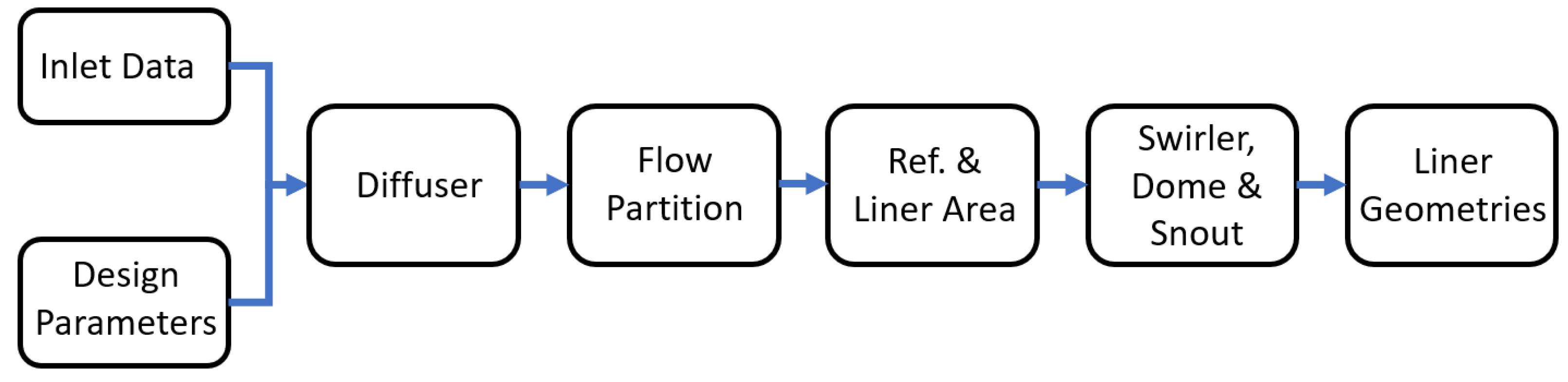
2. Methodology
2.1. Overview
2.2. Modeling Approach
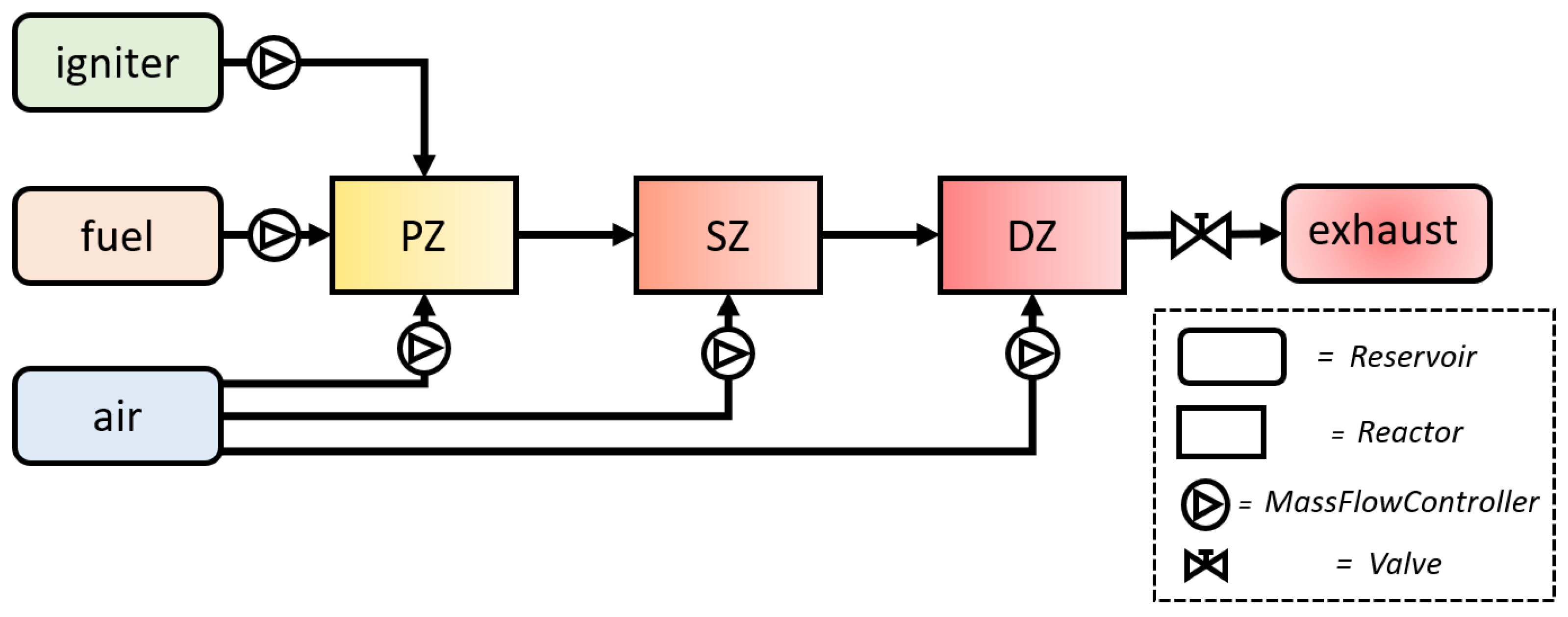
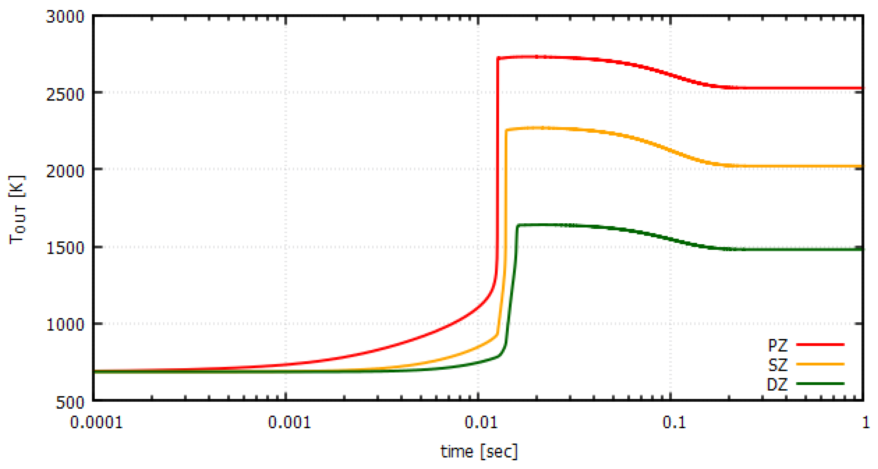
2.3. CRN Formulation and Structure
2.3.1. CRN Virtual Components
2.3.2. Layout
2.3.3. Postprocess
2.4. Model Tuning
3. Verification Examples
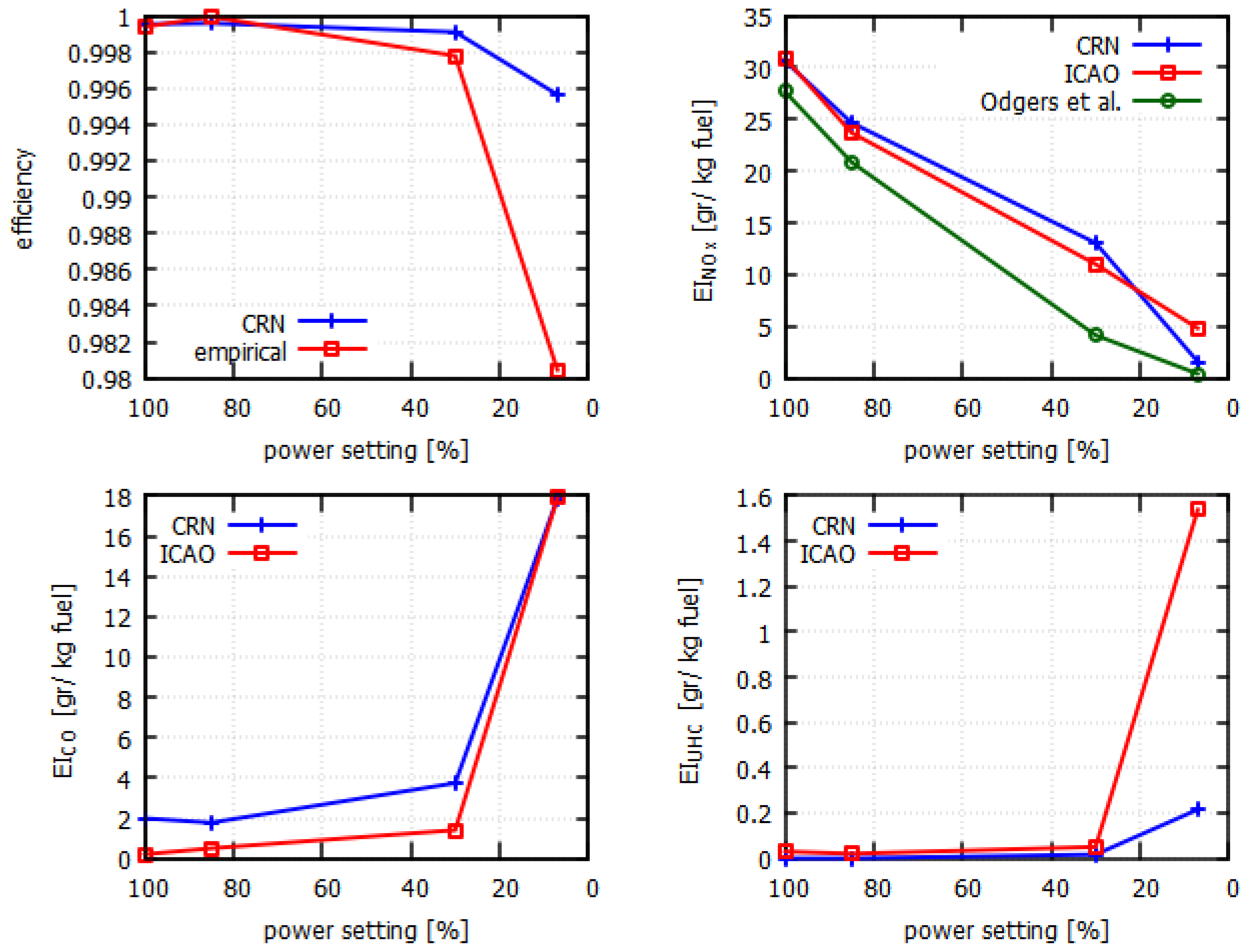
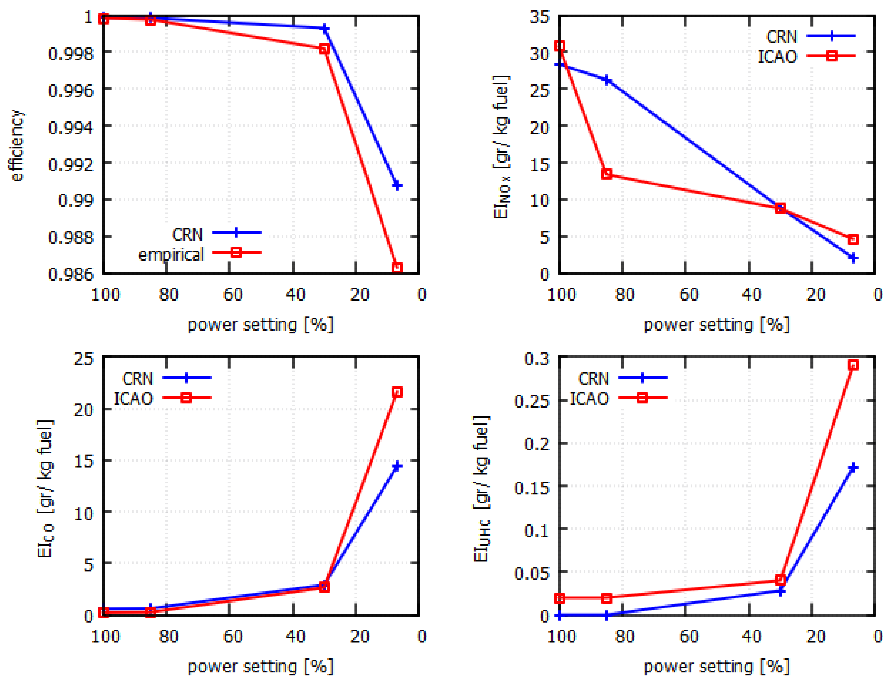
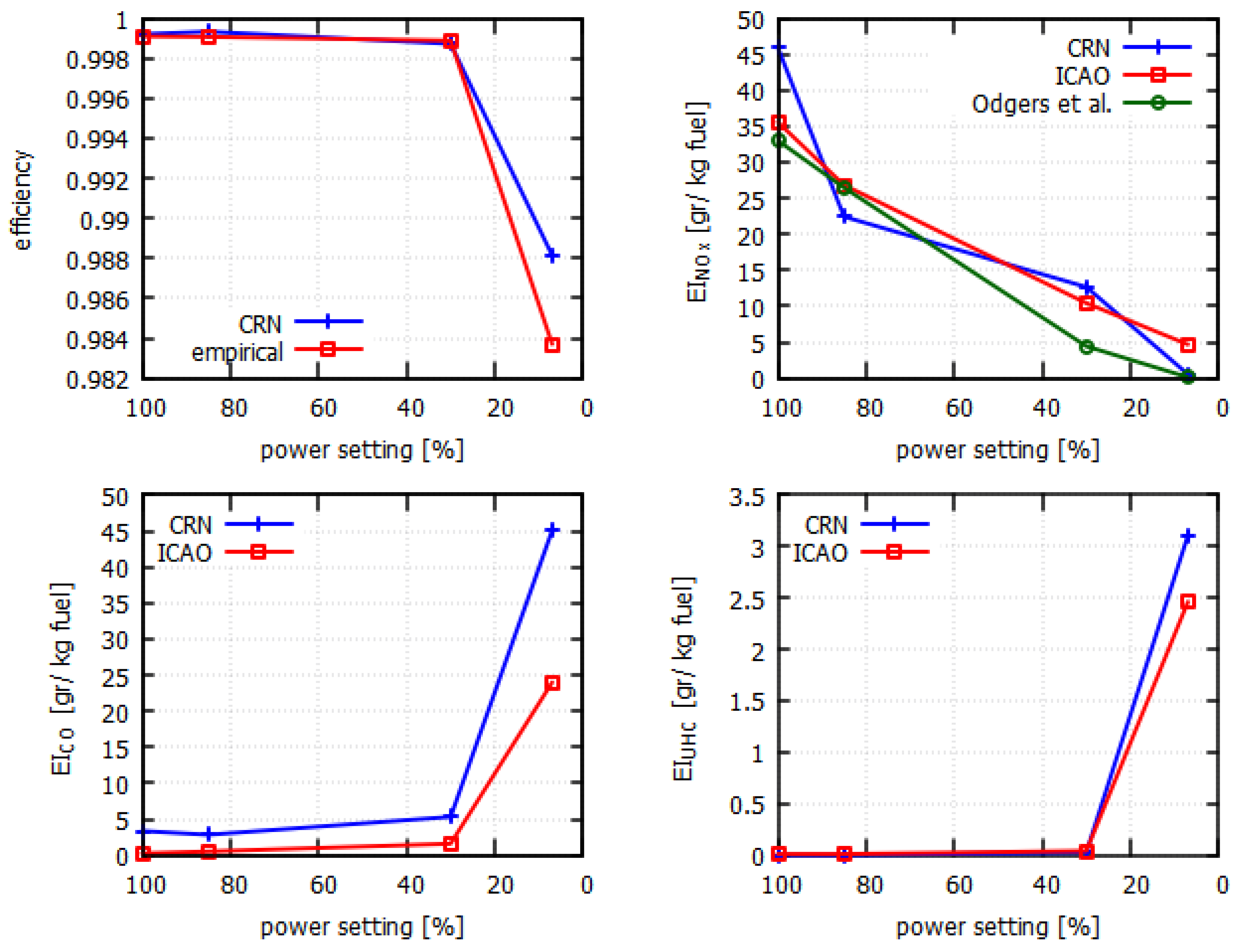
3.1. Engine Test Cases
3.2. Efficiency Study
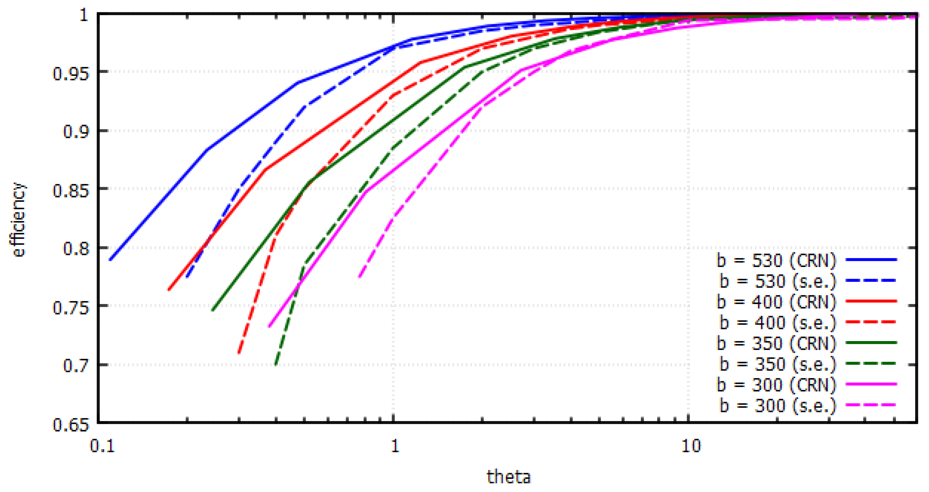
3.2.1. Parametric Analysis
3.2.2. Efficiency Map Generation
4. Preliminary Design
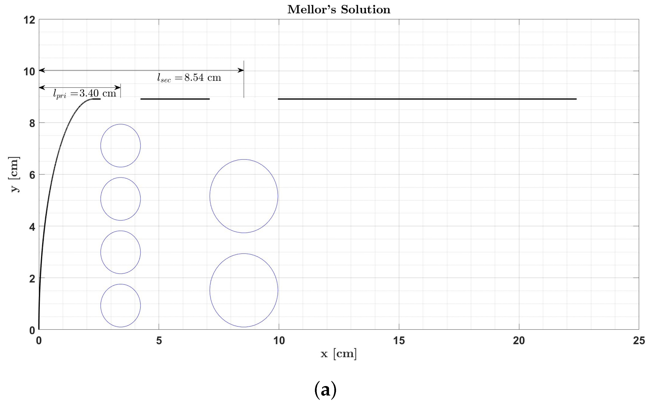
- A correlation algorithm based upon Mellor et al. [32], opting to decrease emissions and keep the emissions constant, yielded a slightly modified geometry, which, in turn, the CRN model evaluated with respect to its landing and take-off (LTO) cycle emissions.
- An optimization loop was employed in which the CRN model was integrated so as to produce optimized LTO cycle emissions.
4.1. Combustor Design Algorithms
4.2. Application
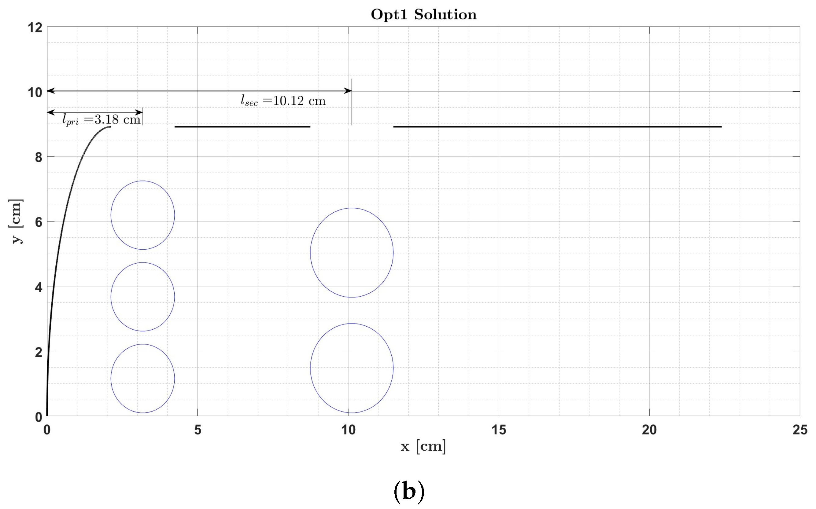
- Opt1: The selected design variables were and at cruise, which are bound between 0.8–1.09 and 0.58–0.8, respectively, as well as the length ratio of the PZ () and the SZ (), which are both bound between 5–70%. The objective was the minimization of the emissions while keeping the emissions unchanged, thus replicating Mellor’s [34] objective.
- Opt2: The selected design variables were exactly the same as the case of Opt1, while the objective was the minimization of all three pollutant emissions: , , and UHCs.
- Opt3: The selected design variables were the ones selected in the cases Opt1 and Opt2, plus L and , which can be modified within a range from their initial value (from the initial design).The objective, as in case Opt2, was the minimization of all three pollutant emissions: , , and UHCs.
5. Discussion and Conclusions
Author Contributions
Funding
Data Availability Statement
Conflicts of Interest
Abbreviations
| GHG | Greenhouse Gas | |
| UHCs | Unburnt Hydrocarbons | |
| SAF | Sustainable Aviation Fuel | |
| CFD | Computational Fluid Dynamics | |
| CRN | Chemical Reactor Network | |
| FAR | Fuel-to-Air Ratio | |
| PFR | Plug Flow Reactor | |
| PSR | Perfectly Stirred Reactor | |
| PaSR | Partially Stirred Reactor | |
| PSRs | Perfectly Stirred Reactor series | |
| PZ | Primary Zone | |
| SZ | Secondary Zone | |
| DZ | Dilution Zone | |
| ICAO | International Civil Aviation Organization | |
| PS | Power Setting | |
| LTO | Landing and Take-Off | |
| Symbol | Description | Units |
| Burner Reference Area | m | |
| * | Air Ratio per Zone—i | - |
| Damkohler number | - | |
| Combustor Total Pressure Losses | - | |
| Emission Index of product—k | gr of k/kg fuel | |
| Fuel-to-Air Ratio | - | |
| h | Enthalpy per unit of Mass | J/kg |
| L | Liner Length | m |
| * | Length Ration per Zone—i | - |
| Lower Heating Value | J/kg | |
| Molar Mass | kg/kmol | |
| Number of Time Steps | - | |
| Combustion Efficiency | - | |
| Number of Moles of species—k | mol | |
| Inlet Total Pressure | Pa | |
| Total Pressure per Zone—i | Pa | |
| Part Load Constant | - | |
| Inlet Air Flow | kg/s | |
| Q | Heat per unit of Mass | J/kg |
| Adiabatic Flame Temperature | Kelvin | |
| Inlet Total Pressure | Kelvin | |
| Total Temperature per Zone—i | Kelvin | |
| Simulation Time | s | |
| Formation Time | s | |
| Molar Fraction of species—k | - | |
| Mass Fraction of species—k | - | |
| Equivalence Ratio | - | |
| Burner Loading Parameter | kg/s | |
Appendix A. Postprocess
Appendix A.1. LHV Calculation
Appendix A.2. Alternative nb Computation Method
- The fraction of moles of , , and per initial fuel mass is defined as follows:
- The fraction of moles of air, , and argon per initial fuel mass is defined as follows:
- The fraction of product gasses per initial fuel mass when assuming complete combustion is defined as follows:
- The actual fraction of product gasses per initial fuel mass for a set initial equivalence ratio is defined as follows:
- The quantities and are computed using the molar functions and , respectively, of the remaining and UHCs at the outlet of the burner after the completion of the combustion simulation of the CRN model:
Appendix B. Engine Cases Thermodynamic and Geometric Data

| CFM56-7B27 | Take-Off | Climb | Approach | Idle | Cruise |
| [K] | 795 | 759 | 619 | 477 | 687 |
| [bar] | 28.50 | 24.80 | 10.75 | 3.78 | 9.67 |
| [kg/s] | 47.47 | 42.80 | 21.33 | 8.32 | 17.35 |
| [-] | 0.026 | 0.024 | 0.016 | 0.014 | 0.022 |
| [%] | 5.01 | 5.14 | 5.53 | 5.24 | 5.02 |
| LEAP-1A26 | Take-Off | Climb | Approach | Idle | Cruise |
| [K] | 819 | 785 | 635 | 513 | 743 |
| [bar] | 32.73 | 28.58 | 13.04 | 4.89 | 12.53 |
| [kg/s] | 35.29 | 32.20 | 17.29 | 6.90 | 14.38 |
| [-] | 0.024 | 0.022 | 0.014 | 0.013 | 0.022 |
| [%] | 4.38 | 4.49 | 4.89 | 4.60 | 4.41 |
| TRENT 772 | Take-Off | Climb | Approach | Idle | Cruise |
| [K] | 858 | 814 | 645 | 496 | 712 |
| [bar] | 36.13 | 31.35 | 14.10 | 5.63 | 11.44 |
| [kg/s] | 121.13 | 109.28 | 57.19 | 26.25 | 42.37 |
| [-] | 0.026 | 0.023 | 0.014 | 0.010 | 0.020 |
| [%] | 5.14 | 5.28 | 5.66 | 5.74 | 5.21 |
| Parameter | CFM56-7B27 | CFM LEAP-1A26 | RR TRENT 772 |
|---|---|---|---|
| [m] | 0.160 | 0.225 | 0.180 |
| L [m] | 0.178 | 0.157 | 0.191 |
| * | 1.057 | 1.090 | 1.024 |
| * | 0.605 | 0.600 | 0.580 |
| 30.82 | 29.14 | 28.46 | |
| 23.02 | 23.80 | 21.78 | |
| 46.15 | 47.05 | 49.76 |
Appendix C. Geometric Data for Initial and Improved Burner Designs
| Parameter | Initial | Mellor | Opt1 | Opt2 | Opt3 |
|---|---|---|---|---|---|
| [m] | 0.155 | 0.155 | 0.155 | 0.155 | 0.148 |
| L [m] | 0.224 | 0.224 | 0.224 | 0.224 | 0.224 |
| * | 0.842 | 0.818 | 0.913 | 1.077 | 1.089 |
| * | 0.656 | 0.639 | 0.605 | 0.589 | 0.580 |
| 38.69 | 39.81 | 35.67 | 30.48 | 29.92 | |
| 10.94 | 11.17 | 18.15 | 25.43 | 26.21 | |
| 20.29 | 15.19 | 14.18 | 19.29 | 35.12 | |
| 19.79 | 22.92 | 30.99 | 48.76 | 41.46 |
References
- Lai, Y.Y.; Christley, E.; Kulanovic, A.; Teng, C.C.; Björklund, A.; Nordensvärd, J.; Karakaya, E.; Urban, F. Analysing the opportunities and challenges for mitigating the climate impact of aviation: A narrative review. Renew. Sustain. Energy Rev. 2022, 156, 111972. [Google Scholar] [CrossRef]
- Marszałek, N.; Lis, T. The future of sustainable aviation fuels. Combust. Engines 2022, 191, 29–40. [Google Scholar] [CrossRef]
- Grewe, V.; Rao, A.G.; Grönstedt, T.; Xisto, C.; Linke, F.; Melkert, J.; Middel, J.; Ohlenforst, B.; Blakey, S.; Christie, S.; et al. Evaluating the climate impact of aviation emission scenarios towards the Paris agreement including COVID-19 effects. Nat. Commun. 2021, 12, 3841. [Google Scholar] [CrossRef] [PubMed]
- Lee, D.S.; Fahey, D.W.; Skowron, A.; Allen, M.R.; Burkhardt, U.; Chen, Q.; Doherty, S.J.; Freeman, S.; Forster, P.M.; Fuglestvedt, J.; et al. The contribution of global aviation to anthropogenic climate forcing for 2000 to 2018. Atmos. Environ. 2020, 244, 117834. [Google Scholar] [CrossRef] [PubMed]
- European Partnership. Clean Aviation: Strategic Research and Innovation Agenda. EU Counc. Regul. 2021, L 427, 17–119.
- Airbus. Cities, Airports & Aircraft. Global Market Forecast. 2019. Available online: https://www.airbus.com/sites/g/files/jlcbta136/files/2021-07/GMF-2019-2038-Airbus-Commercial-Aircraft-book.pdf (accessed on 12 March 2023).
- Liu, Z.; Deng, Z.; Davis, S.J.; Giron, C.; Ciais, P. Monitoring global carbon emissions in 2021. Nat. Rev. Earth Environ. 2022, 3, 217–219. [Google Scholar] [CrossRef] [PubMed]
- Liu, Y.; Sun, X.; Sethi, V.; Li, Y.G.; Nali, D.; Abbott, D.; Gauthier, P.; Xiao, B.; Wang, L. Development and application of a preliminary design methodology for modern low emissions aero combustors. Proc. Inst. Mech. Eng. Part A J. Power Energy 2021, 235, 783–806. [Google Scholar] [CrossRef]
- Schripp, T.; Anderson, B.E.; Bauder, U.; Rauch, B.; Corbin, J.C.; Smallwood, G.J.; Lobo, P.; Crosbie, E.C.; Shook, M.A.; Miake-Lye, R.C.; et al. Aircraft engine particulate matter emissions from sustainable aviation fuels: Results from ground-based measurements during the NASA/DLR campaign ECLIF2/ND-MAX. Fuel 2022, 325, 124764. [Google Scholar] [CrossRef]
- Rezvani, R. A Conceptual Methodology for the Prediction of Engine Emissions. PhD Thesis, Georgia Institute of Technology, Atlanta, GA, USA, 2010. [Google Scholar]
- Mark, C.P.; Selwyn, A. Design and analysis of annular combustion chamber of a low bypass turbofan engine in a jet trainer aircraft. Propuls. Power Res. 2016, 5, 97–107. [Google Scholar] [CrossRef]
- Oliveira, J.; Brojo, F. Simulation of the combustion of bio-derived fuels in a CFM56-3 combustor. In Proceedings of the 2nd International Conference Sustainable and Renewable Energy Engineering, Hiroshima, Japan, 10–12 May 2017; Volume 235, pp. 14–18. [Google Scholar]
- Altarazi, Y.S.M.; Talib, A.R.A.; Yusaf, T.; Gires, J.Y.E.; Ghar, M.F.A.; Lucas, J. A review of engine performance and emissions using single and dual biodiesel fuels: Research paths, challenges, motivations and recommendations. Fuel 2022, 326, 125072. [Google Scholar] [CrossRef]
- Przysowa, R.; Gawron, B.; Białecki, T.B.; Legowik, A.; Merkisz, J.; Jasinski, R. Performance and emissions of a microturbine and turbofan powered by alternative fuels. Aerospace 2021, 8, 25. [Google Scholar] [CrossRef]
- Chiong, M.C.; Chong, C.T.; Ng, J.; Lam, S.S.; Tran, M.; Chong, W.W.F.; Jaafar, M.N.M.; Valera-Medina, A. Liquid biofuels production and emissions performance in gas turbines: A review. Energy Convers. Manag. 2018, 173, 640–658. [Google Scholar] [CrossRef]
- Alexiou, A.; Aretakis, N.; Kolias, I.; Mathioudakis, K. Novel Aero-Engine Multi-Disciplinary Preliminary Design Optimization Framework Accounting for Dynamic System Operation and Aircraft Mission Performance. Aerospace 2021, 8, 49. [Google Scholar] [CrossRef]
- Alexiou, A.; Aretakis, N.; Roumeliotis, I.; Mathioudakis, K. Short and long range mission analysis for a Geared Turbofan with Active Core Technologies. In Proceedings of the ASME Turbo Expo, Glasgow, UK, 14–18 June 2010; Volume 3, pp. 643–651. [Google Scholar]
- Lefebvre, A.H.; Balla, D.R. GAS Turbine Combustion: Alternative Fuels and Emissions; CRC Press: Boca Raton, FL, USA, 2010. [Google Scholar]
- DuBois, D.; Paynter, G.C. ‘Fuel Flow Method2’ for Estimating Aircraft Emissions. SAE Trans. 2006, 115, 1–14. [Google Scholar]
- Glavan, I.; Poljak, I.; Kosor, M. A gas turbine combustion chamber modeling by physical model. Sci. J. Marit. Res. 2021, 35, 30–35. [Google Scholar] [CrossRef]
- Chandrasekaran, N.; Guha, A. Study of prediction methods for NOx emission from turbofan engines. J. Propuls. Power 2012, 28, 170–180. [Google Scholar] [CrossRef]
- Kee, R.J.; Coltrin, M.E.; Glarborg, P.; Zhu, H. Chemically Reacting Flow: Theory and Practice, 2nd ed.; John Wiley and Sons: Hoboken, NJ, USA, 2017. [Google Scholar]
- Xue, R.; Hu, C.; Nikolaidis, T.; Pilidis, P. Effect of Steam Addition on the Flow Field and NOx Emissions for Jet-A in an Aircraft Combustor. Int. J. Turbo Jet. Eng. 2016, 33, 381–393. [Google Scholar] [CrossRef]
- Nozari, M.; Eidiattarzade, M.; Tabejamaat, S.; Kankashvar, B. Emission and performance of a micro gas turbine combustor fueled with ammonia-natural gas. Int. Engine Res. 2022, 23, 1012–1026. [Google Scholar] [CrossRef]
- Renzi, M.; Patuzzi, F.; Baratieri, M. Syngas feed of micro gas turbines with steam injection: Effects on performance, combustion and pollutants formation. Propuls. Power Res. 2017, 206, 697–707. [Google Scholar] [CrossRef]
- EcosimPro|PROOSIS Modelling and Simulation Software. Available online: http://www.proosis.com/ (accessed on 17 July 2023).
- Luche, J. Obtention de Modeles Cinetiques Reduits de Combustion: Application a un Mecanisme du Kerosene. PhD Thesis, Universite D’Orleans, New Orleans, LA, USA, 2003. [Google Scholar]
- Cantera Co. Reactors and Reactor Networks Documentation. Available online: https://cantera.org/science/reactors/reactors.html (accessed on 5 May 2023).
- Walsh, P.P.; Fletcher, P. Gas Turbine Performance, 2nd ed.; ASME Press: New York, NY, USA; Backwell Publishing: Hoboken, NJ, USA, 2004. [Google Scholar]
- EASA|ICAO Aircraft Engine Emissions Databank. Available online: https://www.easa.europa.eu/en/domains/environment/icao-aircraft-engine-emissions-databank (accessed on 6 May 2023).
- Odgers, J.; Kretschmer, D. The Prediction of Thermal NOx in Gas Turbines. In Proceedings of the ASME Turbo Expo, Beijing, China, 1–7 September 1985; Volume 2. [Google Scholar]
- Mellor, A.M.; Fritsky, K.J. Turbine Combustor Preliminary Design Approach. J. Propuls. 1990, 6, 334–343. [Google Scholar] [CrossRef]
- Mattingly, J.D. Aircraft Engine Design, 2nd ed.; AIAA: Reston, VA, USA, 2002. [Google Scholar]
- Mellor, A.M. Design of Modern Turbine Combustor; Academic Press: London, UK, 1990. [Google Scholar]
- Mattingly, J.D. Elements of Propulsion, Gas Turbine and Rockets; AIAA: Reston, VA, USA, 2006. [Google Scholar]


| Initial | Mellor | Opt1 | Opt2 | Opt3 | |
|---|---|---|---|---|---|
| TO | 78.02 | 75.56 | 49.68 | 30.85 | 26.06 |
| Cl | 59.66 | 50.26 | 49.29 | 21.39 | 18.83 |
| Ap | 2.14 | 1.67 | 3.51 | 12.83 | 18.19 |
| Id | 0.31 | 0.20 | 0.47 | 1.47 | 2.09 |
| LTO (gr) | 12,999.3 | 11,469.2 | 10,102.0 | 6090.6 | 6042.0 |
| TO | 1.83 | 1.46 | 1.15 | 1.45 | 1.88 |
| Cl | 1.51 | 1.19 | 1.00 | 1.41 | 1.91 |
| Ap | 2.04 | 2.30 | 2.48 | 3.33 | 3.84 |
| Id | 25.33 | 34.55 | 25.77 | 18.39 | 17.03 |
| LTO (gr) | 5131.0 | 6778.7 | 5129.8 | 3940.2 | 3824.6 |
| TO | 4.0 | 7.0 | 5.0 | 6.0 | 6.0 |
| Cl | 6.7 | 1.1 | 6.7 | 2.6 | 2.2 |
| Ap | 0.040 | 0.052 | 0.036 | 0.015 | 0.013 |
| Id | 2.077 | 3.360 | 1.516 | 0.233 | 0.134 |
| LTO (gr) | 384.0 | 620.5 | 279.9 | 44.4 | 25.7 |
Disclaimer/Publisher’s Note: The statements, opinions and data contained in all publications are solely those of the individual author(s) and contributor(s) and not of MDPI and/or the editor(s). MDPI and/or the editor(s) disclaim responsibility for any injury to people or property resulting from any ideas, methods, instructions or products referred to in the content. |
© 2023 by the authors. Licensee MDPI, Basel, Switzerland. This article is an open access article distributed under the terms and conditions of the Creative Commons Attribution (CC BY) license (https://creativecommons.org/licenses/by/4.0/).
Share and Cite
Villette, S.; Adam, D.; Alexiou, A.; Aretakis, N.; Mathioudakis, K. A Simplified Chemical Reactor Network Approach for Aeroengine Combustion Chamber Modeling and Preliminary Design. Aerospace 2024, 11, 22. https://doi.org/10.3390/aerospace11010022
Villette S, Adam D, Alexiou A, Aretakis N, Mathioudakis K. A Simplified Chemical Reactor Network Approach for Aeroengine Combustion Chamber Modeling and Preliminary Design. Aerospace. 2024; 11(1):22. https://doi.org/10.3390/aerospace11010022
Chicago/Turabian StyleVillette, Sergios, Dimitris Adam, Alexios Alexiou, Nikolaos Aretakis, and Konstantinos Mathioudakis. 2024. "A Simplified Chemical Reactor Network Approach for Aeroengine Combustion Chamber Modeling and Preliminary Design" Aerospace 11, no. 1: 22. https://doi.org/10.3390/aerospace11010022