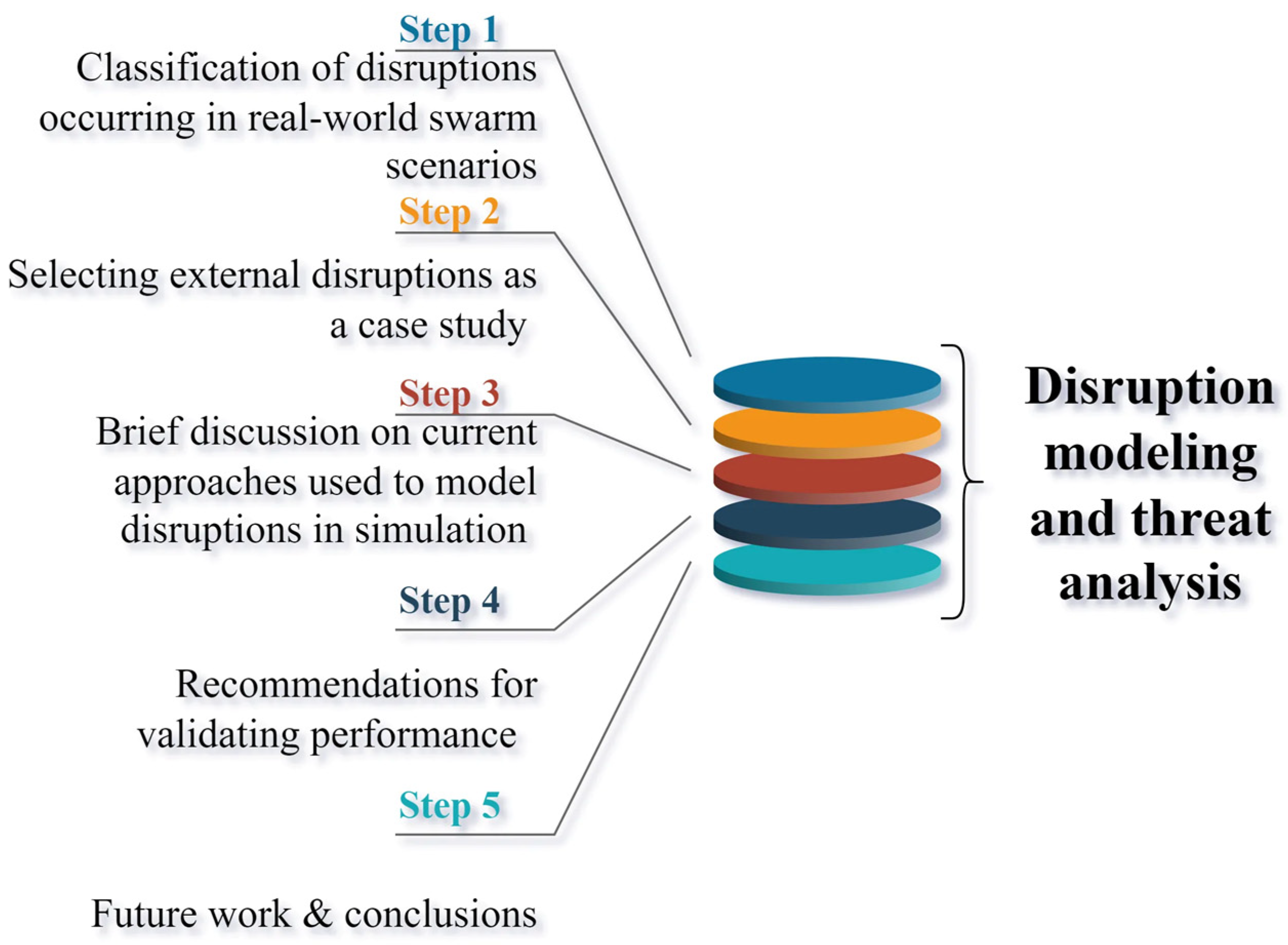
Article

Modeling Wind and Obstacle Disturbances for Effective Performance Observations and Analysis of Resilience in UAV Swarms

by
Abhishek Phadke
1,2,*,
F. Antonio Medrano
1,2,
Tianxing Chu
1,2,
Chandra N. Sekharan
2 and
Michael J. Starek
1,2
1
Conrad Blucher Institute for Surveying and Science, Texas A&M University-Corpus Christi, Corpus Christi, TX 78412, USA
2
Department of Computer Science, Texas A&M University-Corpus Christi, Corpus Christi, TX 78412, USA
*
Author to whom correspondence should be addressed.
Aerospace 2024, 11(3), 237; https://doi.org/10.3390/aerospace11030237
Submission received: 11 February 2024 / Revised: 6 March 2024 / Accepted: 14 March 2024 / Published: 18 March 2024
(This article belongs to the Special Issue UAV System Modelling Design and Simulation)

Abstract

:
UAV swarms have multiple real-world applications but operate in a dynamic environment where disruptions can impede performance or stop mission progress. Ideally, a UAV swarm should be resilient to disruptions to maintain the desired performance and produce consistent outputs. Resilience is the system’s capability to withstand disruptions and maintain acceptable performance levels. Scientists propose novel methods for resilience integration in UAV swarms and test them in simulation scenarios to gauge the performance and observe the system response. However, current studies lack a comprehensive inclusion of modeled disruptions to monitor performance accurately. Existing approaches in compartmentalized research prevent a thorough coverage of disruptions to test resilient responses. Actual resilient systems require robustness in multiple components. The challenge begins with recognizing, classifying, and implementing accurate disruption models in simulation scenarios. This calls for a dedicated study to outline, categorize, and model interferences that can be included in current simulation software, which is provided herein. Wind and in-path obstacles are the two primary disruptions, particularly in the case of aerial vehicles. This study starts a multi-step process to implement these disruptions in simulations accurately. Wind and obstacles are modeled using multiple methods and implemented in simulation scenarios. Their presence in simulations is demonstrated, and suggested scenarios and targeted observations are recommended. The study concludes that introducing previously absent and accurately modeled disruptions, such as wind and obstacles in simulation scenarios, can significantly change how resilience in swarm deployments is recorded and presented. A dedicated section for future work includes suggestions for implementing other disruptions, such as component failure and network intrusion.

1. Introduction

Unoccupied aerial vehicles (UAVs) and their swarming capabilities represent a transformative technology. UAV swarm applications are spread across real-world scenarios, including disaster response [1], military [2], and remote sensing [3]. However, the swarms must maintain an acceptable performance and mission continuity in the face of multiple disruptions in their target environments. Fuzzy rules for systemic resilience define robustness, adaptability, extensibility, and a capability to rebound from highly impacted low-performance states [4]. Researchers propose novel means of resilience integration in UAV swarms at a fast pace. Resilience integration is often application-specific [5]; i.e., only the UAV swarm components that are deemed to require a robust implementation are made so. This is due to the difficulty of creating comprehensive deployments in all components and modules of a swarm system [6] or the high costs and long development timelines.
Comprehensive simulation experiments are a great way to test the proposed implementations without the risk of real-world failures. Thus, disruption and threat modeling are pivotal in UAV and UAV swarm simulation experiments. Without a rigorous understanding of potential disruptions, these agents can be easily compromised, leading to data breaches, loss of assets, or unintended consequences. Not accounting for threats can have dire ramifications in military and security contexts.
Furthermore, UAV swarms, which operate based on inter-UAV communications and collaborative algorithms, pose unique challenges due to their emergent behaviors. Disruption and threat modeling help ensure these behaviors are thoroughly tested against adversarial tactics and natural disturbances. By simulating various threat scenarios, researchers and developers can identify vulnerabilities, devise countermeasures, and ensure the resilience and security of UAV systems, making them safe and efficient for real-world applications. Figure 1 outlines the process followed in this research to classify disruptions, following which wind and obstacles were the two external disturbances selected for further examination. Step 3 involves examining the current work in modeling these disruptions in simulation scenarios. Based on these, simulation scenarios are created that include these modeled disruptions as mathematical models and physical elements. Every scenario has a specific implementation and goal. The UAV swarm performance in every scenario is examined to understand how the presence of disruption elements changes the swarm performance, and the results are presented. Future work for implementing additional classes of disruption, such as component failure and network intrusion, are outlined, followed by concluding remarks.
Figure 2 classifies the major disruptions into six categories. These outline the disruptions a single UAV or a swarm might face during a real-world flight. With advancements in simulation platforms, high-fidelity UAV models, and realistic environment rendering, it is now possible to simulate a broad range of disruptions during the simulation stage. The contributions of this study are as follows:
  • A novel study to evaluate various wind and obstacle disruption modeling methods for UAV operation experiments;
  • A general implementation of wind and obstacle simulation is analyzed using methods to introduce disruption scenarios in simulation environments;
  • Sample scenarios and experiments are designed where different models of each disruption are used, and the results for the observation of swarm performance in the face of the introduced disruptions are discussed.
Representing all potential disruptions accurately in a simulation is currently a challenge due to the simulator platform limitations and the ability to accurately encode the physical reactions of agents to external stimuli. Modeling elements like snow and rain in simulators without express support is tedious. Some simulation platforms, such as the discontinued Microsoft AirSim [7], support rain, snow, and additional weather conditions such as fog and dust. Wind components can be modified together or individually to produce drafts and gusts. Figure 3 depicts an AirSim simulation with a single agent flying in a simulated world with heavy rain and wind weather conditions.
Figure 4 shows the UAV flying in the same environment but with a simulated dust storm. Simulators allow the possibility of testing deployments such as these that would be otherwise difficult to test in real-world situations without risk to hardware and mission progress.
Thus, this study combines a descriptive analysis of various disruptions, suggested methods to implement them as models, and experiments that can be designed to validate swarm performance. The paper is organized as follows: Based on a brief introduction in Section 1, Section 2 outlines how wind can be modeled in simulation experiments. Section 3 does the same for obstacle modeling. Section 4 describes the various scenarios in which the above wind and obstacle modeling can be incorporated. Section 5 analyzes the results produced when the wind and obstacle models are used in the described scenarios. Section 6 outlines future research directions for modeling additional disruptions, such as component failure and network intrusion. Section 7 provides the concluding remarks.

2. Wind Modeling

Wind is an omnipresent factor in aerial flight modeling and one of the most influential forces aerial vehicles experience during motion. It is crucial that we consider the effects of wind during UAV operations. While actual wind forces can be experienced in real-world tests, modeling the impact of wind on UAV swarms for experimental or simulation studies can be challenging due to the complex aerodynamics involved. However, understanding these effects is crucial for various applications, from disaster response to agriculture. Wind factors can also affect fuel consumption, takeoff, landing, basic flight maneuvers, and sensor recordings. More severe effects include the possibility of agents being thrown off course by strong gusts, causing collisions with each other or with environmental obstacles, resulting in cascaded failures. There are several methods in which wind models can be incorporated into simulations, depending on the experiment’s complexity, the simulator’s capabilities, and the needs of the target aircraft and swarm mechanic being tested. Figure 5 lists the various options to simulate wind models.
Wind models can be broadly classified as follows:
  • Mathematical models are further divided into deterministic and stochastic wind models [8,9]. While constant and Gaussian models are subcategories of deterministic models, random walk models fall under the stochastic category;
  • Computational fluid dynamic methods that numerically solve Navier–Stokes equations to simulate fluid flow [10];
  • Data-driven methods rely on real-time or historical wind data that are queued and used as input;
  • Hybrid methods use the above data to create Windfield grids [11] and machine learning (ML) implementations.
The following section briefly outlines the methods to create wind models in simulations. One common approach is to use a deterministic wind model. This model assumes that the wind speed and direction are known at all points in the simulation region. This can be achieved using real-time weather data or by generating a synthetic wind field as a guiding or opposing force. Deterministic wind models are relatively simple to implement and can be used to simulate the effects of wind on a UAV swarm, especially in simulations that do not have them. However, they may not be accurate enough for applications such as those where the swarm can expect complex wind patterns or turbulence. Wind speed variation in different directions may be possible while accounting for UAV orientation using such models. Equation (1) shows a wind vector field used to decompose wind components:
V w r = V w x ( r ) V w y ( r ) V w z ( r )
where r is a position vector in 3D space and V w x r , V w y r , v w z r are wind speed components at position r. The UAV velocity relative to wind VuI at any point r can be calculated as outlined in Equation (2):
V u r = R r · V a V w r
R ( r ) is the rotation matrix representing the aircraft orientation at position r , and V a is the UAV’s airspeed vector. The rotation matrix can be computed based on the UAV altitude or Euler angles, although the latter is more accurate. A more complex gust model can involve multiple gusts in different directions. A 3D gust model is created in Equation (3):
V w t , r = V w o + i = 0 N A i sin 2 π f i t + ϕ i
where N is the number of gust components, Ai and fi are the amplitude and frequency of the i-th gust component, ϕ i is the phase angle, t is time, and r is the position in 3D space. This represents a superposition of multiple gust components in different directions and frequencies.
Another approach is to use a stochastic wind model. This type of model considers the randomness of wind dynamics, which is caused by factors such as weather changes and the presence of obstacles. Stochastic wind models are more complex than deterministic wind models but can more accurately represent realistic wind conditions. An example is shown in Equation (4), with spatiotemporal correlations highlighted:
V ω t , r = μ r + σ r · Z t , r
Here, μ r is the mean wind speed at position r, σ r is the standard deviation of wind speed at position r, and Z t , r is a stochastic process with zero mean and unit variance used to represent random fluctuations through time t. The stochastic component can be correlated in time and space to represent realistic wind variations. Stochastic wind models are often used in applications where it is essential to account for the uncertainty in wind conditions, such as the development of UAV swarms for search and rescue [12] or disaster relief. A random walk stochastic process is represented in Equation (5) using sequential real-world historical data as inputs:
W t = W t 1 + Δ t σ z
where z N 0,1 is a standard Gaussian random variable, σ is the wind volatility, and Δ t is the time increment. Turbulence modeling can also be carried out based on the Kaimal Spectrum for Atmospheric Turbulence [13], a semi-empirical model widely used in wind engineering and applications necessary to consider wind turbulence. Examples include the following:
  • Designing wind turbines and other structures that are exposed to wind loads;
  • Predicting the performance of aircraft and other vehicles that operate in turbulent conditions;
  • Modeling the dispersion of pollutants in the atmosphere.
S ( f ) = 4 σ 2 L 5 / 3 1 + 6 f L / U
Equation (6) for the Kaimal Spectrum has S ( f ) denoting the power spectral density, σ is the turbulence standard deviation, L is the length scale, U is the mean wind speed, and f is the frequency. Computational fluid dynamics (CFD) can model wind flow around and through objects such as buildings, bridges, and wind turbines. It can also model wind flow in complex terrains such as mountains and valleys. However, some disadvantages of using it involve it being numerically complex and computationally expensive and producing results that are sensitive to the choice of the model and the input parameters. The Navier–Stokes equations are the foundation of fluid dynamics and can model wind accurately when solved numerically. They are given in Equation (7):
V t + ( V · ) V = 1 p P + v 2 V + g
where V is the velocity field, p is the fluid density, P is the pressure, v is the kinematic viscosity, and g is the gravitational acceleration. Hybrid models combining the above-established methods with particle filters can also be explored. A particle filter is a sequential Monte Carlo method for tracking the state of a dynamic system from a sequence of noisy measurements. It is a recursive algorithm that maintains a set of weighted samples, called particles, that represent the possible states of the system. The particle filter propagates the particles forward in time according to the system dynamics and then updates their weights based on the latest measurement. Particle filters have been used to predict wind speed and direction for various applications, including wind turbine control, wind power forecasting, and aviation.
The wind’s evolution is represented in Equation (8), where f is a transition model and ε t is a noise term representing the inherent unpredictability in wind evolution:
x t + 1 = f ( x t ) + Ɛ t
N particles are initialized for the wind state, for i = 1… N, where p ( x 0 ) is the initial distribution of the wind state as shown in Equation (9):
x 1 0 p ( x 0 )
For each time step in the simulation, we predict the next state for each particle, as shown in Equation (10):
x i t + 1 = f ( x i t + w t )
where w t q ( w t ) is the process of the noise-capturing wind unpredictability.
Real-world measurements or selective historical data can be used to update particle weights according to Equation (11):
w i t + 1 w i t × P ( z t + 1 | x i t + 1 )
Resample the particles with low weights and, using the weighted particles, generate an ensemble estimate of the wind state and use it in the simulation model as shown in Equation (12):
x t + 1 = i = 1 N w i t + 1 x i t + 1
The estimate x t + 1 represents the wind state that the simulated UAV swarm encounters at time t + 1. By iterating through this process, the PF provides a dynamic wind model that can be refined with new observations and used to inject a realistic wind disturbance into the simulation. Uncertainty in dynamics and sporadically available real-world measurements are especially well-represented in this model. This method can also be incorporated in grid-based maps that consider the impact of neighboring cells and structures while computing the value of a cell. This is true in the real world when wind patterns suggest spatial coherence, e.g., a large weather front moving across the grid. The current literature that details wind disruption modeling includes Article [14], which uses the Dryden wind turbulence model to apply the velocity component of wind to the vehicle, and Article [15], which performs simulation tests for small UAVs in constant wind, wind shear, and propeller vortex scenarios using the Von Karman spectral function, trapezoidal model, and Proctor model, respectively. Article [16] mentions applying turbulence modeling using high-pass and low-pass frequency filters for their application-specific research method.
Simulation modeling may also be highly specific depending on the application and use-case scenario for swarms and individual aircraft. Table 1 lists the recent work that has incorporated wind disturbances in a UAV study in some manner.
In addition to the type of wind model, the following factors and simulation parameter relationships should also be considered when modeling wind for UAV swarm experiments:
  • The altitude of the UAVs: The wind speed and direction can vary significantly with altitude.
  • The size of the UAVs: Smaller UAVs are more affected by wind than larger UAVs.
  • UAV shape and construction: The shape and construction of UAVs (fixed wing, rotary aircraft, etc.) can also affect how they are impacted by wind.
  • The terrain and landcover: The terrain and associated landcover can also affect the wind speed and direction.
The best way to model wind for UAV swarm experiments will depend on the application. However, by considering the factors mentioned above, researchers can develop wind models that are accurate and realistic enough to support the development of safe and reliable UAV swarms.

3. Obstacle Modeling

For swarm experimentation environments, obstacles introduce elements, offering diverse challenges in maintaining the cohesiveness and operational effectiveness of the swarm. Obstacles are extensive in the actual environment and can be classified into static and dynamic entities, each possessing distinct impedimental properties. Static obstacles, immovable and persistently located within the operational space, require the swarm to enact path-planning and collision avoidance algorithms, ensuring that the swarm can navigate these obstacles without jeopardizing inter-agent distances and communication links. On the other hand, dynamic obstacles, characterized by their temporally variable position, velocity, and, potentially, morphology, necessitate the incorporation of predictive modeling, real-time sensory data assimilation, and reactive motion planning in the UAV swarm’s navigational algorithms to uphold spatial integrity and task efficacy.
The mechanical, aerodynamic, and sensorial disruptions imposed by these obstacles could disturb the swarm’s spatial configuration, potentially disrupt communication links, prolong task completion times, and compromise the safety of the UAVs and their operational environment. Consequently, simulating obstacles in a swarm experimental environment serves a twofold purpose: it provides a means to systematically study and understand the intrinsic and emergent behaviors of the swarm in obstacle-riddled environments, and it facilitates the development, validation, and optimization of algorithms under controlled, reproducible, and scalable settings. Integrating various obstacles into simulation environments enables researchers to ascertain UAV swarm algorithms’ robustness, adaptability, and reliability under diverse and challenging conditions. This structured and rigorous approach to obstacle simulation thus underpins the development of resilient, efficient, and safe UAV swarm technologies. Figure 6 outlines the obstacle simulation methods that can be used.
The choice of obstacle implementation method can depend on factors such as the level of experiment design and requirements, factors being studied, model fidelity and constraints, and choice of simulation platform.
Geometric models typically employ mathematical equations to describe shapes in space. Beyond simple shapes, these models can become significantly intricate, encompassing parametric and non-parametric forms. A representation of the geometric obstacle structure is shown in Equation (13). Obstacle models created using super-quadrics [21], and Gielis surfaces are one of the ways to implement intricately controlled obstacles with the freedom to design convex and concave surfaces in simulation environments. This control is significant in studying phenomena such as swarm cohesion and fragmentation [22], where agents can become stuck in obstacle boundaries and lose contact with the swarm.
| x a | 2 m + | 1 b | 2 n + | z c | 2 p = 1
Here, a, b, and c are scale factors along the three axes, and m, n, and p are shape parameters that modulate the degree of the shape. Gielis surfaces can describe a wide array of shapes in a single equation and can be represented in a polar co-ordinate system. An example mathematical description is presented in Equation (14):
r ( ϕ ) = | c o s [ m · ϕ / 4 ] a | 2 n + | s i n ( m · ϕ / 4 ) b | 2 n 1 / n 1
Here, ϕ is the angular parameter, whereas m, a, b, n1, n2, and n3 are shape parameters that formulate various geometric forms. In high-fidelity combinatorial models of wind and obstacles, sharp edges can create more turbulence because they can cause the airflow to separate from the surface, creating vortices. Moreover, most current implementations do not study the effect of deflecting airflows from smooth objects affecting swarms. This can be covered using smooth surfaces, application-specific aerodynamic properties, and deflection forces to check aircraft reactions to tertiary wind effects. Gielis surfaces can be designed to have specific aerodynamic properties. For example, they can be designed to deflect the wind in a specified direction. This can be useful for evaluating the airflow around an object or creating a lift.
Another common approach is to use a manifold to represent the obstacle surface using a mesh of primitive geometry, which is then defined as the obstacle surface. An example would be the use of Riemannian manifolds that resemble Euclidean space [23,24]. The metric tensor field g, described on the manifold M, encodes the intrinsic geometric properties of M. Figure 7 shows examples of a smooth surface and a hyperbolic manifold modeled with the intention of them being obstacles in the simulation scenario. With curved surfaces, natural and unnatural arcs, and curved edges, these models more closely mimic real-world obstacles than current implementations.
Riemannian manifold representations have several advantages over other methods of representing obstacles in simulations. First, they are versatile and can represent various obstacles, from simple geometric shapes to complex natural objects. Second, they are efficient for storage and manipulation, making them suitable for large-scale simulations. Third, they can create dynamic obstacles essential for many simulations. While a singular equation cannot represent manifolds, a sample case for generation is outlined in Equation (15):
d s 2 = g i j ( x ) d x i d x j
where d s is the infinitesimal distance on the manifold, and x = ( x 1 , x 2 , , x n ) denotes co-ordinates on the manifold M and gij(x) are metric tensor components. Additional options include using quadratic surfaces with second-degree equations, which can be manipulated to depict extensive shapes.
Grid-based models, especially occupancy grids, discretize the environment into a grid of cells. Each cell represents a specific region in space and holds a value indicating the likelihood that an obstacle occupies the area. Given an environment of ε of dimensions L × W, it can be discretized into a grid of size m × n where m and n are defined below, and δ is the size of each cell. These dimensions are shown in Equation (16):
m = L δ n = W δ
Each cell Ci,j of this grid will have occupancy probability P(Ci,j), where p ( c i , j ) [ 0,1 ] , p ( c i , j ) = 1 indicates an obstacle exists in that cell, and a value of 0 means the cell is free. Here, i and j indicate the specific cell co-ordinates with respect to the m × n grid. Using the Bayesian Update rule, given a series of measurements, Z = ( z 1 , z 2 , z k ) . The probability of occupancy can be updated as shown in Equation (17):
P ( c i , j | Z ) = P ( z k | c i , j ) × P ( c i , j | z k 1 ) P z k
where P ( c i , j | Z ) is the likelihood of current measurements given the cell’s state, P ( c i , j | z k 1 ) is the prior probability from previous measurements, and P ( z k ) is the evidence of current measurements. Implementation considerations like resolution size, the sensor model characteristics for range, accuracy and noise profile, memory, and the nature of obstacles (static or dynamic) will affect the final results.
One of the advantages of using simulation approaches is the ability to repeatedly test deployed agents in a wide range of random scenarios. This offers a richer variability in the test scenario and the simulation results generated. In terms of swarm control, procedural generation can allow the creation of randomized yet rule-based environments that can challenge and test the robustness of control algorithms. Multiple approaches can be used to accomplish world generation. Prevalent uses are terrain generation using constraints set for the height, width, and variability functions of geographic features such as mountains. A Perlin noise can be used to generate natural-looking patterns [25]. The gradient noise function can generate height maps for terrains where obstacles can be placed at height thresholds. The following Equation (18) can be used as a base to define the ground terrain, where F is the fade function, G is the gradient function, and p represents position:
F ( p ) = ( 1 F ( p ) ) · G ( p ) · ( p P 0 ) + F ( p ) · G ( p + δ P ) · ( p p 0 δ P )
Using the above definition, this study generated examples of procedurally generated noise-defined terrain with different height fields, as represented in Figure 8. These methods can often supplement additional methods based on need and simulation platforms, such as rule-based object placement, where their placement can also be controlled and algorithmically defined obstacle dimensions. Modern simulation platforms also support importing mesh-based models as objects in the simulation scene. These objects are then recognized as single or multiple objects in a scene, depending on the complexity required and scene resources to record agent events such as collisions and other physical reactions. Like wind models, the presence of obstacles and methods of simulating them may vary highly from study to study, depending on the use-case scenario. At the same time, a brief bibliometric and perspective trend analysis based on data obtained in [26] revealed that the number of relevant research works that consider and simulate obstacles is more numerous than the research that considers wind modeling as a disturbance. While a summary of the extracted results derived during the bibliometric analysis is shown in Figure 9, Table 2 lists some recent investigations in the year range of 2022–2023 that have incorporated obstacle models in their swarm research. Table 3 has studies conducted in the same time range that incorporate wind and obstacles as disturbances.

4. Scenario Modeling for Disruption Occurrence

The following section outlines scenarios modeled using disturbances that can be adopted to enhance a simulation designed to test agent and swarm performance. Scenario and simulation design are essential steps in the performance evaluation process. Every UAV swarm resiliency study models a disruption scenario to test the efficacy of their methodology. It is challenging to argue about the merits of a particular method without comprehensively testing it in an adversarial environment.

4.1. Wind Disruption Scenarios

Wind disruption modeling was examined in three different scenarios explicitly designed to accommodate the variety of ways in which a UAV swarm might be tested: a two-dimensional (2D) area exhibiting opposing forces as a means to include wind effects in existing simulations, a three-dimensional (3D) cross-sectional differential channel wind model to test swarm movement in different orientations, and a close contact formation control situation where generated air effects from one agent may affect other agents. Table 4 outlines the scenario designs created to test wind disruptions and their suitability in various current and future implementations. Scenario 1.1 and 1.2 used instances of UAV agents represented as a point mass, and scenario 1.3 uses actual quadcopter models.
Scenario 1.1 deals with creating wind values in a generated region of interest (ROI) for practical experiments involving agents in 2D space. Wind value cells in simulations can be created in different ways. While a polygonal division of grids is common practice, it can be computationally intensive to incorporate large numbers in a grid simultaneously. A second method uses particles to denote wind force values and their direction to create accompanying or opposing wind directions. This method can better control and represent wind’s stochastic nature and turbulence effects. Figure 10 shows the two described approaches using polygons and particles over an ROI.
Another approach is to use the generated grid values in the space and assign a wind force value to each. An accurate representation of wind flows around structures can be carried out by defining the wind values of cells, mainly around generated obstacles. Effective channel creation is also possible in such scenarios. This is shown in Figure 11, where a specific scenario is illustrated. The grid-based ROI has obstacles denoted by green squares. A wind channel, indicated by the solid red lines, is created, and wind force values for the cells are shown as a text overlay.
Scenario 1.2 implements a PEWFG, shown in Figure 12, which involves simulating a dynamic environment where particles within a grid act as points in a vector field, each exerting forces that mimic wind-like effects on moving agents. This represents a wind field where the wind’s direction and strength vary spatially, providing a realistic simulation environment.
Scenarios 1.1, 1.2, and 1.3 are implemented in MATLAB R2023b. This grid is first implemented in a MATLAB scenario where particles are visualized in a 3D space. At the core of the PEWFG are the particles, each with their properties and behaviors. These particles are defined by their position and velocity within the grid and generate forces characterized by magnitude and direction. The forces can be either repulsive or attractive depending on the simulation and experiment requirements. Each particle affects agents within a specified radius range of influence. A force calculation function governs the interaction between the particles and the agents. This function calculates the force exerted on an agent based on the distance between the agent and the particle. The total force experienced by an agent is the vector sum of the forces exerted by all particles within its vicinity.
The grid structure is adaptable; for example, while it is typically configured as a three-dimensional lattice, it can be modified to a two-dimensional structure or an irregular form to suit specific application needs. The particles within this grid can either have static positions or exhibit dynamic behavior, moving according to predefined patterns or in response to external stimuli. Furthermore, parameters such as the interaction radius, force constants, and decay exponents are tunable based on the application’s specific requirements.
Scenario 1.3, called downwash disruption modeling, is a less-explored area during the formation control of swarm systems. Few studies have examined the effects of close formation agents on each other during formation. The impact of downwash on the UAV altitude has been noted in the current work [39]. While robust formation controls ensure the maintenance of a minimum distance between agents that are often assumed to be greater than the distance between agents required for the downwash effect to come into play, it is essential to note that wind turbulence can influence agents and overcome any feedback mechanisms in place to the controller to overwhelm set constraints.
Most induced airflow and downwash modeling is concerned with single UAV experiments and analysis in agricultural applications, where the downwash plays a significant role in the spread of droplets [40] and plant studies. Downwash affecting airborne sensor readings has been noted in the relevant literature [41], which makes it essential to model it as a disruption for agent operations. Figure 13 shows two agents placed one above another in a CoppeliaSim [42] environment. The bottom agent faces uncertain drift in its movement due to the downwash effects of the agent above it. The four subplots indicate the progression of the simulation, and their perceived order can be concluded from the numbering present in each subplot.
Modern-day physics engines can be integrated into simulation platforms to model the generalized airflow and rigid body reactions, which can further be used to demonstrate the downwash phenomena and their effects in swarm systems. Scenario 1.3 measures the approximate relation between agent distances in parallel trajectories and the influence of downwash on agents below one another, leading to a potential loss of control, energy expenditure, and degradation in the collected sensor data quality. This phenomenon is realized in real-world experiments as well. Figure 14 shows the downwash experienced by the UAV agent circled in red from the agent directly above it.

4.2. Obstacle Scenario Modeling

This section outlines obstacle modeling scenarios based on the methods listed in previous sections. Table 5 summarizes the scenarios with their experiment process for disruption modeling and situations where they can be suitably accommodated.
Scenario 2.1 outlines a simple object creation in a 2D or 3D space to conduct an initial performance assessment of any proposed methodology for multi-agent systems such as area coverage, obstacle avoidance, and energy usage during task completion. Here, a simple constraint-based model for obstacle creation is given where every obstacle has lower and upper bounds defined for dimensions. Obstacle placement is random to initiate the possibility of multiple scenarios. Collisions between agents and obstacles are detected using a masking strategy that records agent co-ordinates concerning obstacle co-ordinates for that particular instance, and a match in co-ordinates would indicate a collision. Figure 15 shows five UAV agents moving in a 3D space with dense obstacles. The cubes denote obstacles, and the red points represent agents moving in the space and attempting to cover it entirely in an allotted time. The four subplots in Figure 15 show the agents’ progression as they move through the simulation time. The order of the subplots is top left, top right, bottom left, and bottom right to get a sense of simulation progression. Some agents may not be visible in the figure as obstacles in the dense map cover them.
Scenario 2.2 extends the realistic experiment scenario where obstacles are modeled to closely mirror the complex geometric constructions in natural environments. Additionally, a wind model was introduced using turbulence generators, such as in [43], to compare the results for obstacle avoidance, path length, and time to consensus. Artificial gust scenarios were created that were set to materialize at 50% of the generated obstacles at random for every simulation instance. Scenario 2.2 has smooth obstacles generated using Gielis surfaces as the supporting framework. A swarm of five agents moving in the 3D map is shown in Figure 16. The agents are denoted as red dots in the map environment.
The following scenario is based on using existing platforms for modeling and testing. Taking advantage of simulation platforms that support higher-level obstacle modeling, a more realistic environment than the one portrayed in Scenarios 2.1 and 2.2 can be created, as shown in Scenario 2.3.
Using CoppeliaSim v4.5 [42], a complete 3D urban environment was created with various obstacles and properties more likely to exist in a natural environment. Each obstacle is individually assigned a profile characteristic that determines the size and speed. A top-down view of the designed scenario is shown in Figure 17. Multiple different obstacles, each with their own set of characteristics, are also present in this scenario.
Table 6 shows the range of obstacles in the map that were modeled, along with their characteristics. A swarm of agents in a mission must make multiple alterations to the path and altitude, so testing the underlying control mechanisms in a variable environment is necessary.

5. Scenario Model Tests and Results

In this disruption modeling study, the objective of the described scenarios is to assist in measuring the operational characteristics of swarms in the face of the implemented disruptions, observe the disruption scenario modeling process, and discuss its potential implications on the current swarm implementations. For the scenarios created above, experiments are designed to validate the presence of disruptions and agents’ behavior in the modeled disruptions. The above section described six scenarios with their own characteristics, objectives, and agents. For validation, each scenario had a use case where it was used in an experiment. While individual scenarios and their experiments are described in their respective sections for wind and obstacles below, Table 7 outlines the scenario numbers with their major and minor disruptions and their dimensionality. Table 8 lists the properties of the UAV agents used in each scenario and their swarm connection type.

5.1. Wind Disruption Scenario

Every scenario in this study is modeled to be tested in an experiment. Table 9 outlines the experiments designed around the disruption scenarios and their significant objectives.
For Experiment 1, a sample run of the wind field grid with obstacles and two agents is shown in Figure 18. Grid values with static single force accompanying or opposing values in 2D will not produce a noticeable drift in the agent path. This can be overcome by introducing feedback in the controller that measures the force values of a cell and performing an exploratory analysis of other cells to find lower-value cells where the agent can move. Another approach is to assume a knowledge-based scenario where agents have prior information on wind values in cells and choose the lowest-value path that maintains obstacle avoidance and swarm cohesion. These disruptions measure the time to reach the destination, overall or last agent time, degree of swarm cohesion maintained during flight, and inter-agent connections. Additionally, since the force values and path chosen can directly affect the time an agent takes to move across the area, a direct relation to the amount of fuel required may also be established and examined.
Figure 19 shows the noticeable change in agent trajectories when agents fly in a no-disruption scenario vs. when they fly in the designed 1.1 simulation with obstacles and a wind field. The 2D deviations in the path trajectory on a smaller scale are shown in Figure 20, where the deviation is measured as the Euclidian distance between the set waypoint and the actual waypoint for the same timestamp.
The variability of deployment using Scenario 1.2 is represented in Figure 21. This shows the possibility of deploying agents around the constructed wind channel grid to observe the targeted phenomena in multiple ways. A 3 UAV agent system is chosen for illustrative purposes. Instance A deploys agents laterally across the completed grid in a manner that exposes them to crosswind channels of different wind speeds. Sub-scenario B puts the agents in a tailwind, traveling through a single wind speed channel. Sub-scenario C has the agent movement opposite the direction of wind flow, creating a single wind speed headwind situation. Sub-scenario D creates a wider deployment where swarm agents face a headwind situation, but, because of a broader flight path, different agents in the same swarm face different wind speeds. In this manner, various experiment variations can be studied using a single wind grid to understand the interactions.
Scenario 1.2 uses similar approaches to measuring the above-outlined metrics, but this time in 3D. This is important since turbulence effects may be prone to change with altitude shifts in agents. Figure 22 uses the SwarmLab [43] simulation platform and the Olfati–Saber [16] flocking implementation to examine the agent transversal time in turbulent wind and obstacles. Both parameters can be modified to explore additional instances.
A single agent was tested in turbulence and no-turbulence scenarios to examine the path changes, deviations, and energy consumption. The tests were conducted over multiple iterations to obtain the average energy consumption metrics and individual results. Figure 23 shows the subplots for a single agent moving in the obstacle space five times in turbulent and non-turbulent scenarios. In addition to the increased path deviations observed in the turbulence scenario, minor crude observations can also be made. For example, the agent movement in the z plane was limited to a smaller range in the non-turbulence scenario because of lesser drift occurring without wind.
Figure 24 shows the agent’s energy expenditure in simple units when moving across the map for each iteration in turbulence and non-turbulence scenarios. Since the experiment was performed five times, five separate readings were recorded. The average energy expended across simulations shows the difference between energy requirements by the agent when simple obstacle avoidance and additional turbulence adjustments are required.
Figure 25 shows path records for the five UAV agents moving in the sparse map for a single iteration in turbulence and non-turbulence scenarios. Their energy consumption records are depicted in Figure 26.
Scenario 1.3 deals with instantaneous forces generated by aerial agents when moving through mission space. While multiple studies acknowledge the unpredictable and unwanted deviation in the agent path and movement in close formation, few studies quantify the effects these might have on the time taken to traverse environments and the additional energy expenditure. Additionally, the current work is lacking in presenting the number of collisions with other agents due to such path deviations. The path deviations of the agent below it are recorded using the bullet physics engine [44] and a pre-set trajectory for two agents flying near a simple downwash profile acting from the center of the agent above.
Figure 27 presents a simulated scenario showing a fixed trajectory for two agents moving in close proximity, one above the other. It is used as a case scenario to model and observe path deviations in agents due to downwash. The path deviation can be recorded along with the total energy spent in trajectories that include deviations vs. those that do not; energy modeling profiles may provide accurate results. For a swarm of agents recording a fundamental movement in a constrained area, the swarm quadcopter deployment in Scenario 1.3b from [45] was adopted, where the size of the constrained area was kept the same. Still, the number of collisions was recorded in two scenarios for 50 simulation instances. The first experiment ran 50 simulation instances where collisions due to drift in agents after proximity were not accounted for, and the second experiment does account for them. An increased number of collisions in the second experiment scenario is observed, as outlined in Figure 28.

5.2. Obstacle Disruption Scenario

Table 10 lists the experiment numbers and the modeled scenarios that they use.
For Experiment 4, a constrained 3D space was filled with a series of randomly placed obstacles, and five agents were set to move in the obstacle space to achieve maximum area coverage within a set time limit. At the initialization of the scene, when the obstacles are generated, a location table is generated that contains information on the presence of obstacles in that simulation instance. This information is accessible by the agents throughout the mission, and the obstacle-checking policy employed by each agent is simple. The next point in the trajectory is checked for the presence of obstacles. If an obstacle is confirmed in that space, an alternate trajectory point is generated by moving in any four lateral and vertical directions available to the agent in 3D space. Every agent is allotted an area to cover within the set time limit. Figure 29 shows the amount of area coverage achieved by an agent on the Y-axis when the probability of an obstacle being present in the following generated point is on the X-axis. A relation can be observed between the area covered by the agent decreasing as the probability of obstacles present increases. The decrease in area coverage is because the agents spend additional time on obstacle avoidance and circumvention, leaving less time for area coverage.
Since the study maintains that the most accurate results for swarm interactions in simulation environments are produced in the presence of accurately modeled wind and swarm disruptions, a combination experiment is designed that involves Scenarios 1.2 and 2.2. These are shown in Experiment 5 in the form of two variations. Experiment 5.1 studies the presence of complex obstacles in 2D and 3D space to showcase the occurrence of swarm disruption phenomena. The effects of wind on agents have not been studied here. Figure 30 shows a view of Experiment 5.1 for testing the avoidance of complex obstacles. Complex obstacles in this scenario are categorized by ragged edges, tapering tops, and non-uniform concave crevices. The agents are denoted by red dots in the map environment.
Figure 31 shows a 2D scenario. Two iterations of the scenario are shown. One has simple circular obstacles, and the other has cross-shaped obstacles with crevices.
The second variation of Experiment 5, 5.2, also implements the previously designed wind Scenario 1.2 that superimposes the 3D space with wind. The swarm cohesion metric is a measure used to analyze the co-ordination and behavior of swarms. It provides insights into how individual agents of the swarm interact with each other and contribute to the overall structure. Often modeled using the inter-agent distance as a base, it can consider other complex models, such as the network strength between agents, velocity matching, and agent heading. The swarm cohesion metric is often a vital indicator of how agents behave during swarm operations such as formation control and obstacle avoidance and can indicate issues such as flock fragmentation. In this case, the swarm cohesion metric is modeled as a function of the distance between agents and the network connections between them.
The distance factor measures the average or median distance between all pairs of agents within the swarm. A smaller average distance indicates a higher spatial cohesion, suggesting that the swarm maintains its formation effectively. Equation (19) represents the mathematical formulation where d i j is the distance between agents i and j for a swarm of N agents, and the average distance D is calculated as shown:
D = 1 ( N 2 ) i = 1 N 1 . j = i + 1 N d i j
The network connection strength factor quantifies the communication or interaction strength between agents. This could be based on the signal strength, the number of communication links, or the reliability of these links. Here, c i j represents the connection strength between agents i and j with values normalized between 1 and 0, where 1 indicates the strongest connection. The average connection strength C across the swarm is defined as shown in Equation (20):
C = 1 ( N 2 ) i = 1 N 1 . j = i + 1 N c i j
Combining these factors, the swarm cohesion metric S is a function that balances the importance of the distance and network connectivity. A linear approach is the simplest design for this, where the weights ω d and ω c reflect the distance and connections. In Equation (21), D m a x represents the normalization factor that is the maximum acceptable average distance in the formation and the sum of the weights to 1. These can be dynamically adjusted to reflect the changing priorities between spatial and communication cohesion.
S = ω d ( 1 D D m a x ) ω c C
Figure 32 shows the changing swarm cohesion values for agents for different case scenarios involving no disruptions, only obstacles, and obstacles and wind disturbance. The best, worst, and average performance are indicated for each case. Cohesion values decrease on the introduction of disturbances, with the worst performance in the scenario with obstacles and wind.
For Experiment 6, the 3D environment is an ideal location to observe various agent and swarm behaviors and their interaction with obstacles and each other. Here, a dispersion phenomenon was observed where agents take off from a common point and move across the map to designated points of interest. While the swarm collectively functions by staying in active communication, each agent has autonomy in path selection and navigation. In dense urban environments such as this, the disruptions experienced by each swarm agent may vary in number, characteristic, and intensity, affecting the agent’s performance, energy consumption, and time taken to reach the goal.
Figure 33 shows the path the three agents took during an active dispersion activity. The colored lines indicated the path taken by the agents to navigate the obstacle environment. Figure 34 shows a viewpoint of the 3D scenario and multiple feeds of the agent FOV of the three agents moving toward their individual goals.
Creating such high-variability and model-based simulation environments is vital for testing the performance of any designed swarm control and resiliency mechanism before actual real-world deployment. Figure 35 shows the encounter rates recorded for various obstacles when a three-agent swarm performed a mission in the simulated environment. The advantage is the ability to run these experiments multiple times with different agents. Additionally, scenes can be created depending on the target environment in the real world.
Table 11 summarizes the results observed for each experiment as a result of the modeled scenarios and induced disruptions.

6. Future Research Directions for Additional Disruption Modeling

The number of possible disruptions that aerial vehicles may face in a real-world environment is numerous. Consequently, disruption modeling and threat analysis is a broad domain. It is challenging to cover all potential disruptions comprehensively in one study. In an attempt to cover the most likely disruption types, this section covers some additional disruptions, suggested ways to model them, and future research directions.

6.1. Motor and Rotor Malfunctions

This article focuses on wind and obstacles; the next section outlines some disruptions the authors plan to address in a prospective study: swarm network intrusion and internal component malfunctions. Component failures due to issues such as overheating, collisions, degradation, and other weather conditions are some of the reasons that these causes cannot be overlooked during simulation modeling. There are multiple approaches to how component failure can be simulated, and resilient implementations and fault tolerance can be tested. Once the base agent model is created, faults can be introduced in particular blocks to generate responses by the agent. Figure 36 shows a UAV block diagram with a focus on motor dynamics. Such models also allow flexibility depending on n, which is the number of motors the vehicle has.
In control systems like the one in the diagram in Figure 36, simulating motor and rotor failure is crucial for studying the system’s resilience and formulating appropriate response strategies. To simulate a rotor failure within this block diagram, one can introduce a fault injection mechanism within the “Motor Dynamics” block or directly after the dynamic functional block. This mechanism can be programmed to completely interrupt a specific motor’s command signal or degrade its performance to simulate partial failures. When the fault is activated, the respective motor would not produce the expected thrust, leading to an imbalance in the UAV’s dynamics. This disturbance is then captured by the “UAV state” block, which would reflect altered motion states such as skewed velocities or angular deviations. The “dynamic functional block” would detect these discrepancies, as the UAV’s current motion would diverge from the desired reference signals. The proportional integral derivative (PID) controller would then minimize the error by adjusting the commands sent to the remaining functioning rotors to stabilize and maintain control of the UAV. Engineers can observe the UAV’s behavior under rotor failure conditions through simulations and develop algorithms to improve its fault tolerance and safety.
Based on the agent model above, a general process for examining faults is shown in Figure 37. The mathematical or block-based diagram is created on a platform such as MATLAB Simulink. Fault injection is carried out using additional blocks to mimic specific scenarios. Simulated data reactions for the rotor during a rotations per minute (RPM) check can be recorded and examined to determine the validity of real-time pose checks before agent takeoff. Figure 38 shows a rotor RPM check conducted before takeoff, and the malfunctioning rotor data are recorded.
Platforms such as the MATLAB UAV toolbox and Simulink package support the photorealistic observation of an agent landing after the simulation of a rotor fault. Figure 39 shows the turn of events that occur after a rotor failure based on the module of the UAV in-flight recovery package provided by MathWorks [46]. The red circle shows the progression of the UAV agent as it falls. The subplots should be viewed from left to right, top row, followed by left to right bottom row.
A range of possible implementations can be proposed once accurate disruption conditions are created. For example, the above module is configured to create a controlled roll and pitch minimum velocity descent using a tuned controller to ensure agent and environment safety.

6.2. Network Intrusion

Network intrusion modeling also opens various avenues for creating and observing accurate disruptions and their effects. Broadly, the approach to recreating network disturbances can be classified in two ways, summarized in Figure 40. The first approach uses a dataset of past network activity as a basis. Essential information from these data is isolated, and a sequential input is created. Popular platforms such as NetLogo [47] or OMNETT++ can accept such data as a model for defined network behavior, such as a flying ad hoc network (FANET). These agents then recreate the network behavior using the provided data. The proposed approach for network security, such as a mobile intrusion detection system (IDS) or a blockchain-assisted security implementation, can be run on the platform to observe the method’s effectiveness. The second approach uses object- or constraint-based models that create stochastic simulations upon which the proposed learning method can act and produce results.
Figure 41 depicts a network study experiment executed in line with the methodology outlined in Figure 40. OMNETT++ 6.0.2 was used as the base platform where a swarm of five UAV agents was assigned an area coverage mission, as shown in Figure 42.
A ground-originated network intrusion attempt was set to execute across the mission area at random locations for each simulation instance. The top plot in Figure 42 shows one example where the agents flew into the mission area for 600 time steps, and each agent experienced intrusion attempts. The intrusion attempts were modeled as discrete events where a ground entity attempts to access agents using a query approach with an agent identification key not in each vehicle’s list of active agent identifiers. Upon detecting such an attempt, the UAV records the location of the intrusion attempt on the map. The bottom plot of Figure 42 shows the number of intrusion attempts each UAV experiences for 50 simulation instances. The location of each attempt for all the cases is collectively modeled as a heatmap in Figure 43. The model disruption’s accuracy can be modified using the other approach, where a dataset of transpired network events is used in terms of simulation time, and a range of network incidents can be examined. While, in this preliminary work, the location and map dimensions of this experiment do not mirror the real world, such applications have a broad range of applications in mapping high-level threat zones and examining the feasibility of vehicular network security:
  • Additional disruptions that can be modeled are task reassignment, where discrete events such as the ones studied above are used to measure task reassignment costs in terms of time, computational resources, and success rates;
  • Evaluating the performance of learning-based approaches for decision making using disruptions modeled to introduce variations to events that the proposed approaches have been trained on can lead to observations of new failure situations or even evolutionary performance by the learning-based approach;
  • Another possible approach is exploring expanding swarms to include heterogeneity, which may add disruptions. Land or water-based vehicles may experience terrain, varied obstacles, and synchronization issues with aerial vehicles.
UAV swarms and their constituent individual agents have to comply with local and international regulations that may be enforced based on their operational area. The recent mandate by the FAA [48,49] enforces the presence of a remote identification (RID) module on all UAV agents in a specific weight class. This RID module is responsible for the open broadcast of operator- and aircraft-identifying information. This may have particular implications on swarm applications, performance, and disruption modeling [50]. The module’s energy consumption is another factor to consider while estimating fuel usage. Additionally, network throughput may be affected by broadcast protocols. Intrusion detection and network security will need modifications to account for the additional agent and operator information available to malicious entities.

7. Conclusions

In conclusion, this research outlines the importance of accurately modeling disruptions in a UAV simulation environment. Through a descriptive review and scenario-based simulations, the study demonstrated that realistic disruption models are essential for accurately assessing UAV performance and reliability in real-world scenarios. These models are not just academic exercises but vital tools in preparing UAV systems to face the unpredictable challenges encountered in operational environments, ranging from weather anomalies to unexpected technical failures. Our findings emphasize that, by integrating comprehensive disruption models, UAV simulations can provide more reliable data, thus enabling researchers and operators to anticipate and mitigate potential issues before they manifest in the field. This proactive approach is critical in ensuring the safety, efficiency, and effectiveness of UAV operations, especially in sensitive applications such as disaster response, surveillance, and logistics. It also paves the way for future studies to explore the development of even more sophisticated and nuanced disruption models. Such advancements could lead to highly adaptive UAV systems capable of real-time response to many environmental and technical variables. In summary, the development and integration of accurate disruption models in UAV simulations is not just an enhancement but an essential step toward realizing the full potential of UAV technologies in various applications. This work establishes the current practices and offers a foundation for future innovation and refinement in UAV systems, swarm design, and operation.

Author Contributions

Conceptualization, A.P. and C.N.S.; investigation, A.P.; writing—original draft preparation, A.P.; visualization, A.P. and T.C.; writing—review and editing, F.A.M., T.C. and M.J.S. All authors have read and agreed to the published version of the manuscript.

Funding

This research received no external funding.

Data Availability Statement

The data presented in this study are available on request from the corresponding author.

Conflicts of Interest

The authors declare no conflicts of interest.

Abbreviations

The following abbreviations are used in this manuscript:
APFArtificial potential field
FOVField of view
FANETFlying ad hoc network
GMTGround moving target
PEWFGParticle effect wind field grid
PIDProportional integral derivative
ROIRegion of interest
RPMRotations per minute
RIDRemote identification
sUASSmall unoccupied aircraft system
UAVUnoccupied aerial vehicle

References

  1. Xiong, T.; Liu, F.; Liu, H.; Ge, J.; Li, H.; Ding, K.; Li, Q. Multi-Drone Optimal Mission Assignment and 3D Path Planning for Disaster Rescue. Drones 2023, 7, 394. [Google Scholar] [CrossRef]
  2. Gans, N.R.; Rogers, J.G. Cooperative Multirobot Systems for Military Applications. Curr. Robot. Rep. 2021, 2, 105–111. [Google Scholar] [CrossRef]
  3. Nagasawa, R.; Mas, E.; Moya, L.; Koshimura, S. Model-based analysis of multi-UAV path planning for surveying postdisaster building damage. Sci. Rep. 2021, 11, 18588. [Google Scholar] [CrossRef]
  4. Woods, D.D. Four concepts for resilience and the implications for the future of resilience engineering. Reliab. Eng. Syst. Saf. 2015, 141, 5–9. [Google Scholar] [CrossRef]
  5. Abhishek, P.; Medrano, F.A. Examining application-specific resiliency implementations in UAV swarm scenarios. Intell. Robot. 2023, 3, 436–461. [Google Scholar] [CrossRef]
  6. Phadke, A.; Medrano, F.A. Towards Resilient UAV Swarms—A Breakdown of Resiliency Requirements in UAV Swarms. Drones 2022, 6, 340. [Google Scholar] [CrossRef]
  7. Shah, S.; Dey, D.; Lovett, C.; Kapoor, A. AirSim: High-Fidelity Visual and Physical Simulation for Autonomous Vehicles. In Proceedings of the Field and Service Robotics, Proceedings of the 11th Conference on Field and Service Robotics, Zürich, Switzerland, 13–15 September 2017; Springer: Cham, Switzerland, 2017. [Google Scholar] [CrossRef]
  8. Loukatou, A.; Howell, S.; Johnson, P.; Duck, P. Stochastic wind speed modelling for estimation of expected wind power output. Appl. Energy 2018, 228, 1328–1340. [Google Scholar] [CrossRef]
  9. Monbet, V.; Ailliot, P.; Prevosto, M. Survey of stochastic models for wind and sea state time series. Probabilistic Eng. Mech. 2007, 22, 113–126. [Google Scholar] [CrossRef]
  10. Toja-Silva, F.; Kono, T.; Peralta, C.; Lopez-Garcia, O.; Chen, J. A review of computational fluid dynamics (CFD) simulations of the wind flow around buildings for urban wind energy exploitation. J. Wind. Eng. Ind. Aerodyn. 2018, 180, 66–87. [Google Scholar] [CrossRef]
  11. Mann, J. Wind field simulation. Probabilistic Eng. Mech. 1998, 13, 269–282. [Google Scholar] [CrossRef]
  12. Phadke, A.; Medrano, F.A. Increasing Operational Resiliency of UAV Swarms: An Agent-Focused Search and Rescue Framework. Aerosp. Res. Commun. 2024, 1, 12420. [Google Scholar] [CrossRef]
  13. Kaimal, J.C.; Wyngaard, J.C.; Izumi, Y.; Coté, O.R. Spectral characteristics of surface-layer turbulence. Q. J. R. Meteorol. Soc. 1972, 98, 563–589. [Google Scholar] [CrossRef]
  14. Choi, H.S.; Lee, S.; Ryu, H.; Shim, H.; Ha, C. Dynamics and Simulation of the Effects of Wind on UAVs and Airborne Wind Measurement. Trans. Jpn. Soc. Aeronaut. Space Sci. 2015, 58, 187–192. [Google Scholar] [CrossRef]
  15. Wang, B.H.; Wang, D.B.; Ali, Z.A.; Ting Ting, B.; Wang, H. An overview of various kinds of wind effects on unmanned aerial vehicle. Meas. Control 2019, 52, 731–739. [Google Scholar] [CrossRef]
  16. Chu, T.; Starek, M.J.; Berryhill, J.; Quiroga, C.; Pashaei, M. Simulation and Characterization of Wind Impacts on sUAS Flight Performance for Crash Scene Reconstruction. Drones 2021, 5, 67. [Google Scholar] [CrossRef]
  17. Tegicho, B.E.; Geleta, T.N.; Bogale, T.E.; Eroglu, A.; Edmonson, W.; Bitsuamlak, G. Effect of Wind on the Connectivity and Safety of Large Scale UAV Swarms. In Proceedings of the 2021 IEEE International Black Sea Conference on Communications and Networking (BlackSeaCom), Bucharest, Romania, 24–28 May 2021; pp. 1–6. [Google Scholar]
  18. Jayaweera, H.M.P.C.; Hanoun, S. Path Planning of Unmanned Aerial Vehicles (UAVs) in Windy Environments. Drones 2022, 6, 101. [Google Scholar] [CrossRef]
  19. Liu, Z.; Xiang, L.; Zhu, Z. Cooperative Standoff Target Tracking using Multiple Fixed-Wing UAVs with Input Constraints in Unknown Wind. Drones 2023, 7, 593. [Google Scholar] [CrossRef]
  20. Azid, S.I.; Ali, S.A.; Kumar, M.; Cirrincione, M.; Fagiolini, A. Precise Trajectory Tracking of Multi-Rotor UAVs Using Wind Disturbance Rejection Approach. IEEE Access 2023, 11, 91796–91806. [Google Scholar] [CrossRef]
  21. Smith, N.E.; Cobb, R.G.; Baker, W.P. Incorporating Stochastics into Optimal Collision Avoidance Problems Using Superquadrics. J. Air Transp. 2020, 28, 65–69. [Google Scholar] [CrossRef]
  22. Olfati-Saber, R. Flocking for Multi-Agent Dynamic Systems: Algorithms and Theory. IEEE Trans. Autom. Control 2006, 51, 401–420. [Google Scholar] [CrossRef]
  23. Bloch, A.; Camarinha, M.; Colombo, L.J. Dynamic interpolation for obstacle avoidance on Riemannian manifolds. Int. J. Control 2019, 94, 588–600. [Google Scholar] [CrossRef]
  24. Bhattacharya, S.; Ghrist, R.; Kumar, V. Multi-robot coverage and exploration on Riemannian manifolds with boundaries. Int. J. Robot. Res. 2013, 33, 113–137. [Google Scholar] [CrossRef]
  25. Le, T. Procedural Terrain Generation Using Perlin Noise; Graduate Project, California State Polytechnic University: Pomona, CA, USA, 2023. [Google Scholar]
  26. Phadke, A.; Medrano, F.A.; Sekharan, C.N.; Chu, T. An analysis of trends in UAV swarm implementations in current research: Simulation versus hardware. Drone Syst. Appl. 2024, 12, 1–10. [Google Scholar] [CrossRef]
  27. Phadke, A.; Antonio Medrano, F.; Chu, T. Engineering resiliency in UAV swarms–A bibliographic analysis. J. Phys. Conf. Ser. 2022, 2330, 012007. [Google Scholar] [CrossRef]
  28. Zhang, C.; Yao, W.; Zuo, Y.; Wang, H.; Zhang, C. Robust Multiple Unmanned Aerial Vehicle Network Design in a Dense Obstacle Environment. Drones 2023, 7, 506. [Google Scholar] [CrossRef]
  29. Wakabayashi, T.; Suzuki, Y.; Suzuki, S. Dynamic obstacle avoidance for Multi-rotor UAV using chance-constraints based on obstacle velocity. Robot. Auton. Syst. 2023, 160, 104320. [Google Scholar] [CrossRef]
  30. Puente-Castro, A.; River, D.; Pedrosa, E.; Pereira, A.; Lau, N.; Fernandez-Blanco, E. Q-Learning Based System for Path Plannig with UAV swarms in Obstacle Environment. arXiv 2023, arXiv:2303.17655. [Google Scholar]
  31. Lin, Y.; Na, Z.; Feng, Z.; Lin, B.; Lin, Y. Dual-game based UAV swarm obstacle avoidance algorithm in multi-narrow type obstacle scenarios. EURASIP J. Adv. Signal Process. 2023, 2023, 118. [Google Scholar] [CrossRef]
  32. Fu, X.; Zhi, C.; Wu, D. Obstacle avoidance and collision avoidance of UAV swarm based on improved VFH algorithm and information sharing strategy. Comput. Ind. Eng. 2023, 186, 109761. [Google Scholar] [CrossRef]
  33. Hao, G.; Lv, Q.; Huang, Z.; Zhao, H.; Chen, W. UAV Path Planning Based on Improved Artificial Potential Field Method. Aerospace 2023, 10, 562. [Google Scholar] [CrossRef]
  34. Liu, X.; Yan, C.; Zhou, H.; Chang, Y.; Xiang, X.; Tang, D. Towards Flocking Navigation and Obstacle Avoidance for Multi-UAV Systems through Hierarchical Weighting Vicsek Model. Aerospace 2021, 8, 283. [Google Scholar] [CrossRef]
  35. Zhang, Z.; Zhang, D.; Kong, D.; Wang, Y. Real-Time Local Obstacle Avoidance and Trajectory Tracking Control of Quadrotor UAVs with Suspended Payload in Complex Environments. IEEE Access 2023, 11, 144017–144029. [Google Scholar] [CrossRef]
  36. Huang, P.; Tang, Y.; Yang, B.; Wang, T. Research on Scenario Modeling for V-Tail Fixed-Wing UAV Dynamic Obstacle Avoidance. Drones 2023, 7, 601. [Google Scholar] [CrossRef]
  37. Chodnicki, M.; Siemiatkowska, B.; Stecz, W.; Stępień, S. Energy Efficient UAV Flight Control Method in an Environment with Obstacles and Gusts of Wind. Energies 2022, 15, 3730. [Google Scholar] [CrossRef]
  38. Zhang, X.; Ding, W.; Wang, Y.; Luo, Y.; Zhang, Z.; Xiao, J. Bio-Inspired Self-Organized Fission–Fusion Control Algorithm for UAV Swarm. Aerospace 2022, 9, 714. [Google Scholar] [CrossRef]
  39. Ferrera, E.; Alcantara, A.; Capitan, J.; Castano, A.R.; Marron, P.J.; Ollero, A. Decentralized 3D Collision Avoidance for Multiple UAVs in Outdoor Environments. Sensors 2018, 18, 4101. [Google Scholar] [CrossRef]
  40. Zhu, Y.; Guo, Q.; Tang, Y.; Zhu, X.; He, Y.; Huang, H.; Luo, S. CFD simulation and measurement of the downwash airflow of a quadrotor plant protection UAV during operation. Comput. Electron. Agric. 2022, 201, 107286. [Google Scholar] [CrossRef]
  41. Hu, J.; Wang, T.; Yang, J.; Lan, Y.; Lv, S.; Zhang, Y. WSN-Assisted UAV Trajectory Adjustment for Pesticide Drift Control. Sensors 2020, 20, 5473. [Google Scholar] [CrossRef]
  42. Rohmer, E.; Singh, S.P.N.; Freese, M. CoppeliaSim (formerly V-REP): A Versatile and Scalable Robot Simulation Framework. In Proceedings of the IEEE/RSJ International Conference on Intelligent Robots and Systems, Tokyo, Japan, 3–7 November 2013; pp. 1321–1326. [Google Scholar]
  43. Soria, E.; Schiano, F.; Floreano, D. SwarmLab: A Matlab Drone Swarm Simulator. In Proceedings of the 2020 IEEE/RSJ International Conference on Intelligent Robots and Systems (IROS), Vegas, NV, USA, 24 October 2020–24 January 2021; pp. 8005–8011. [Google Scholar]
  44. Bullet Real-Time Physics Simulation. Available online: https://pybullet.org/wordpress/ (accessed on 10 February 2024).
  45. Erskine, J. Quadrotor Swarms Simulink. 2020. Available online: https://github.com/JulianErskine/QuadrotorSwarmsSimulink (accessed on 10 February 2024).
  46. MathWorks. UAV Inflight Failure Recovery. Available online: https://www.mathworks.com/help/slcontrol/ug/uav-quadcopter-controller-tuning-and-inflight-failure-recovery.html (accessed on 10 February 2024).
  47. Tisue, S.; Wilensky, U. NetLogo: Design and implementation of a multi-agent modeling environment. In Proceedings of Agent; Springer: Cham, Switzerland, 2004. [Google Scholar]
  48. FAA. Remote Identification of Unmanned Aircraft-Final Rule. 2023. Available online: https://doi.org/2021-08/RemoteID_Final_Rule.pdf (accessed on 10 February 2024).
  49. FAA. UAS Remote Identification. Available online: https://www.faa.gov/uas/getting_started/remote_id (accessed on 10 February 2024).
  50. Phadke, A.; Boyd, J.; Medrano, F.A.; Starek, M. Navigating the skies: Examining the FAA’s remote identification rule for unmanned aircraft systems. Drone Syst. Appl. 2023, 11, 1–4. [Google Scholar] [CrossRef]
Figure 1. The study process followed.
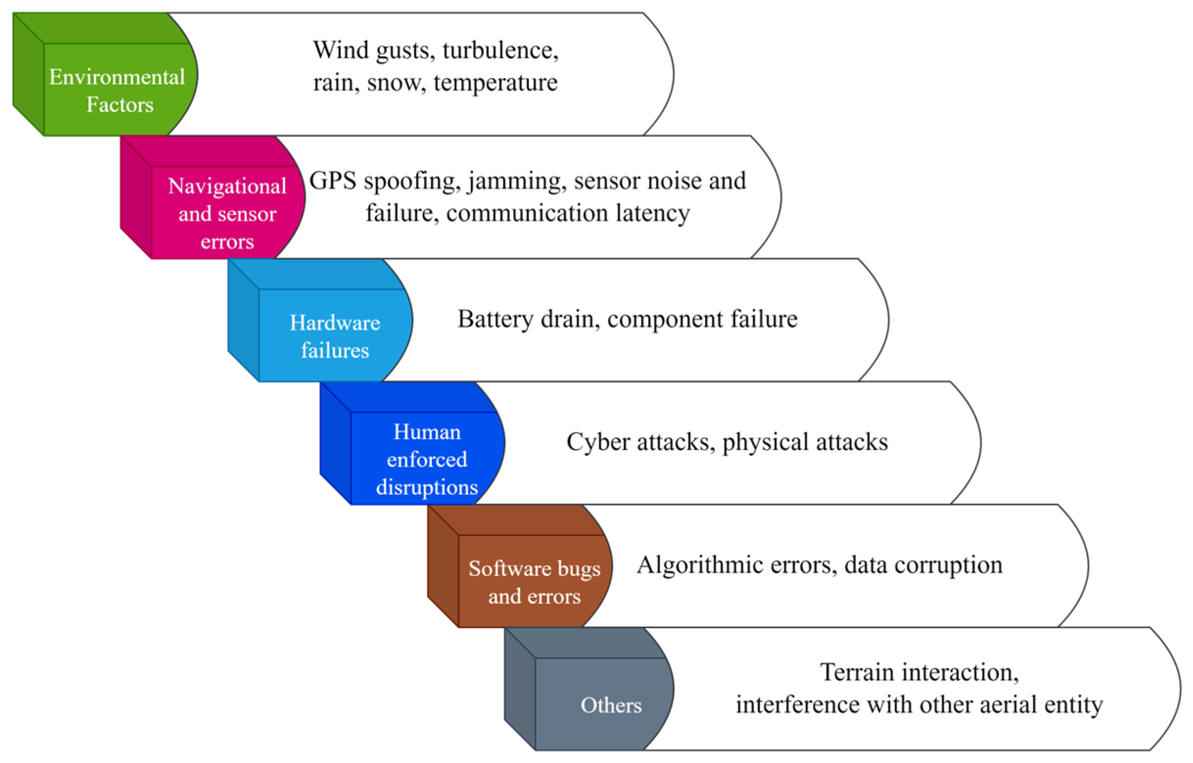
Aerospace 11 00237 g001
Figure 2. A classification of all disruptions in the UAV operating environment.
Aerospace 11 00237 g002
Figure 3. A UAV is shown flying in a simulated Microsoft AirSim environment with rain and wind components. An enlarged view of the setting pane is also shown.
Aerospace 11 00237 g003
Figure 4. A simulated environment with a dust storm and on-board camera field of view (FOV).
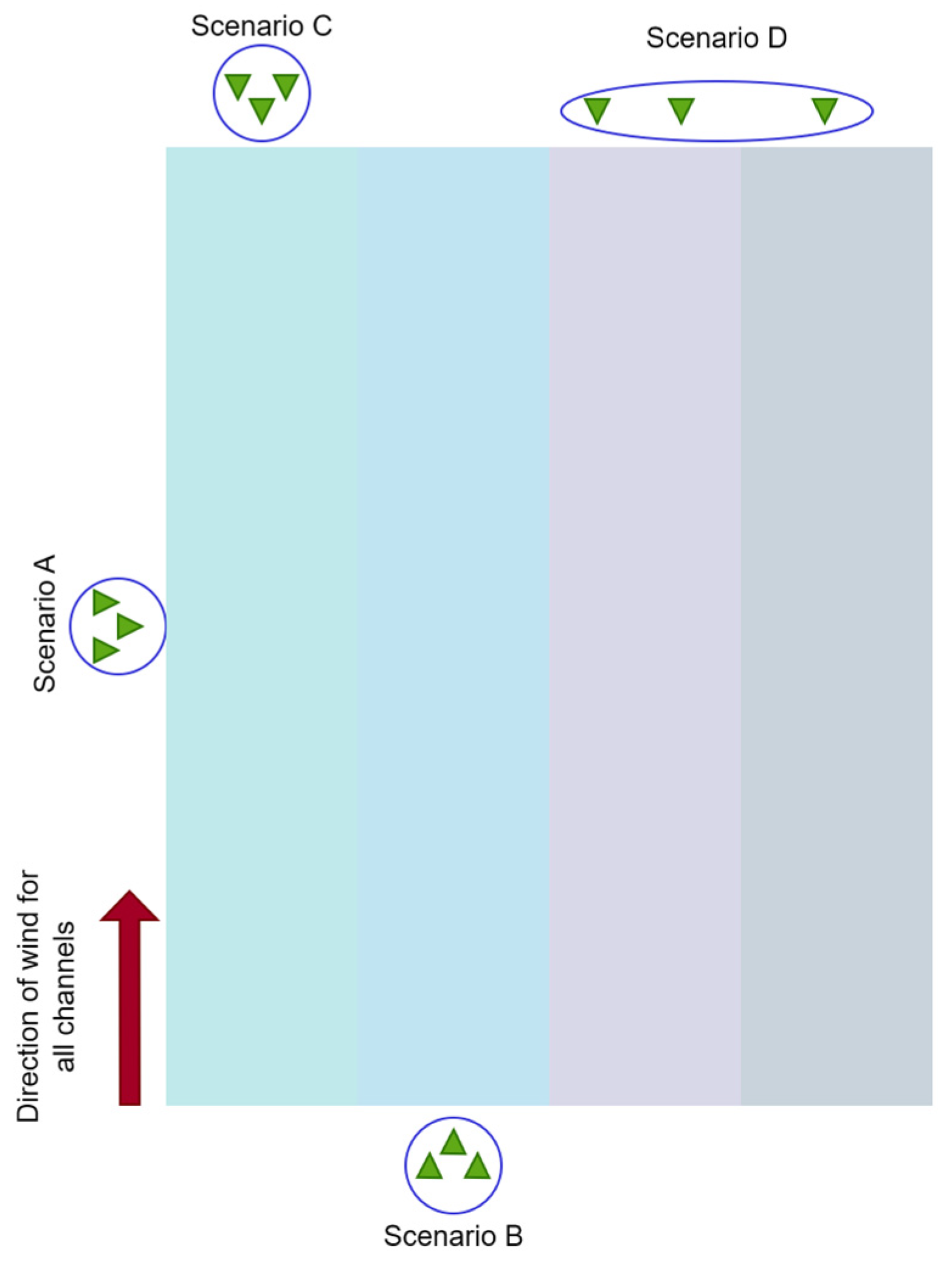
Aerospace 11 00237 g004
Figure 5. A brief overview of methods for modeling the effects of winds in UAV simulations.
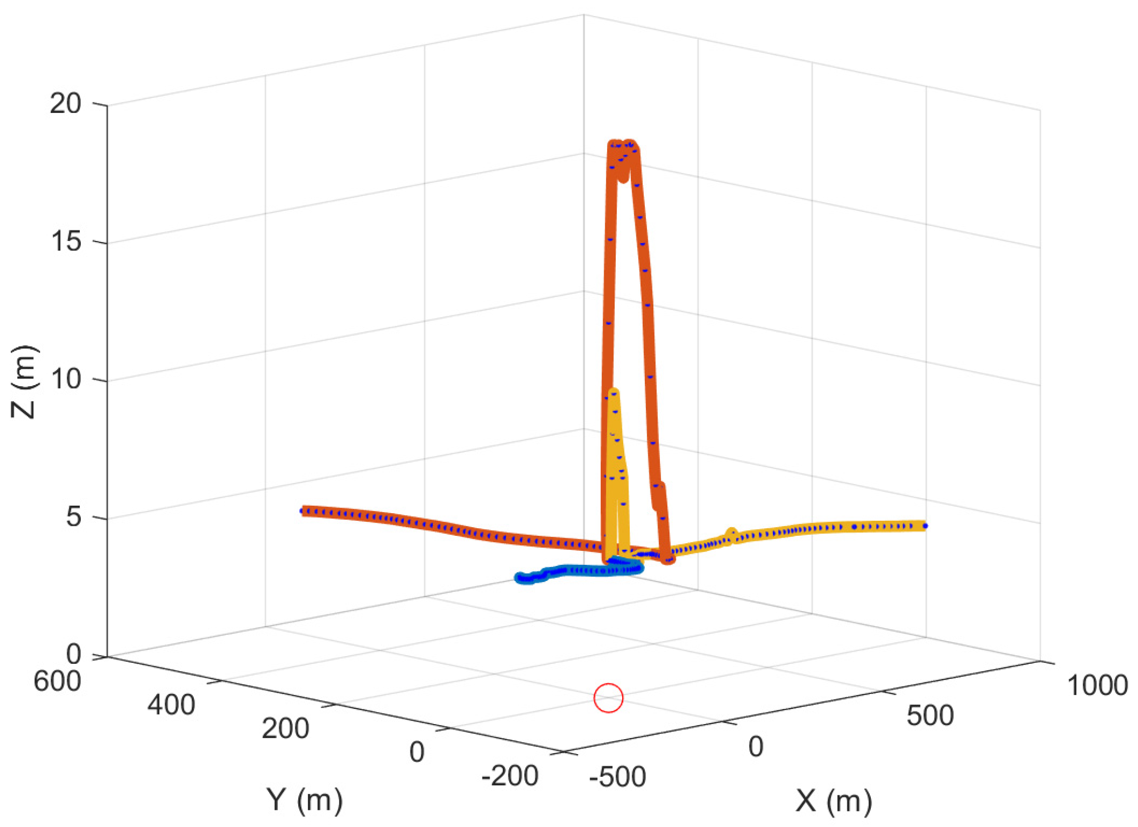
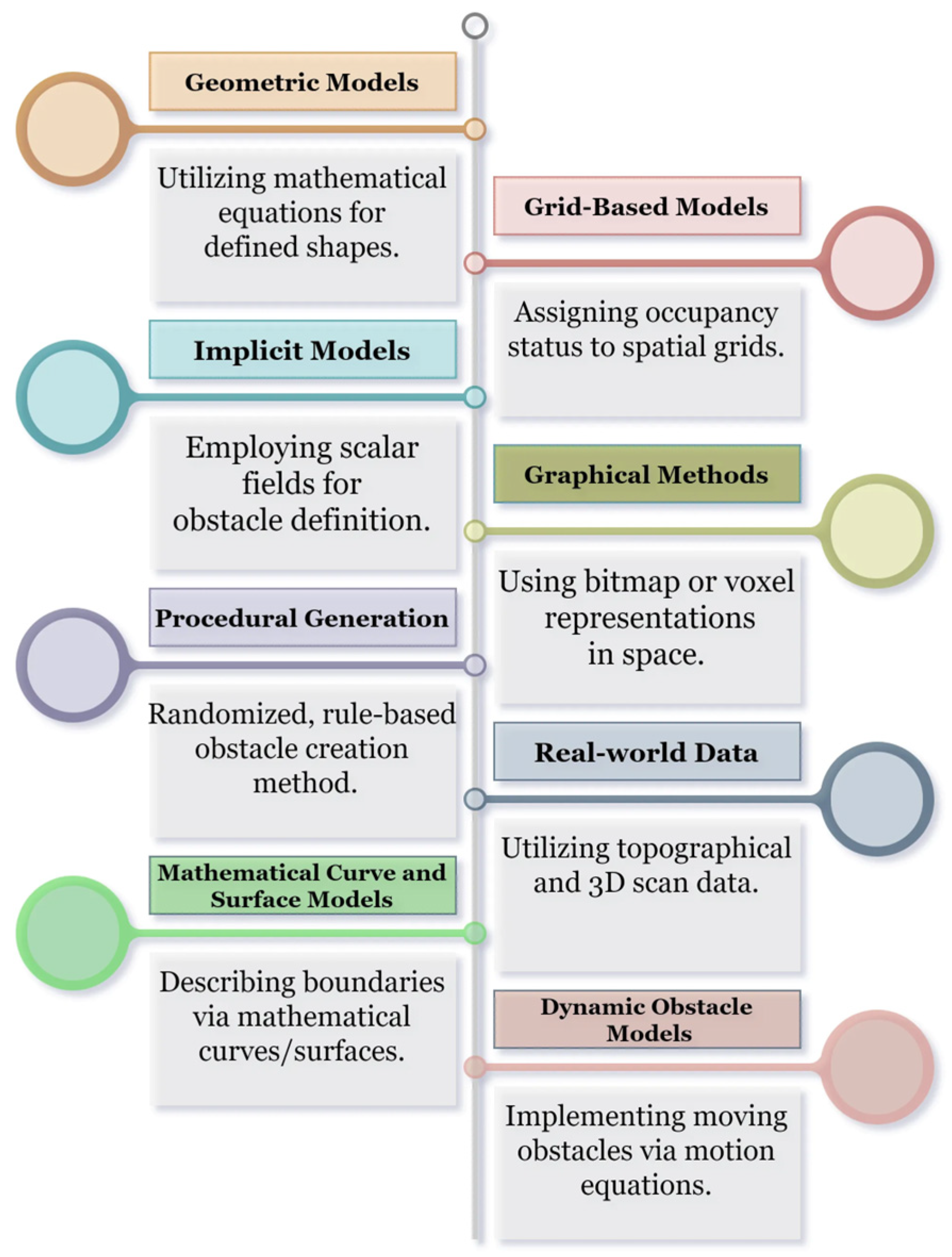
Aerospace 11 00237 g005
Figure 6. An overview of obstacle modeling in simulation scenarios.
Aerospace 11 00237 g006
Figure 7. A Gielis surface obstacle beside a hyperbolic riemannian geometry obstacle.
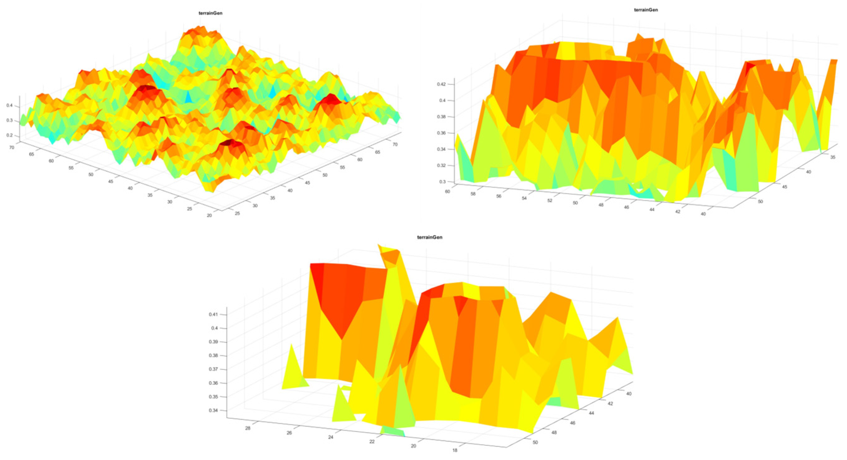
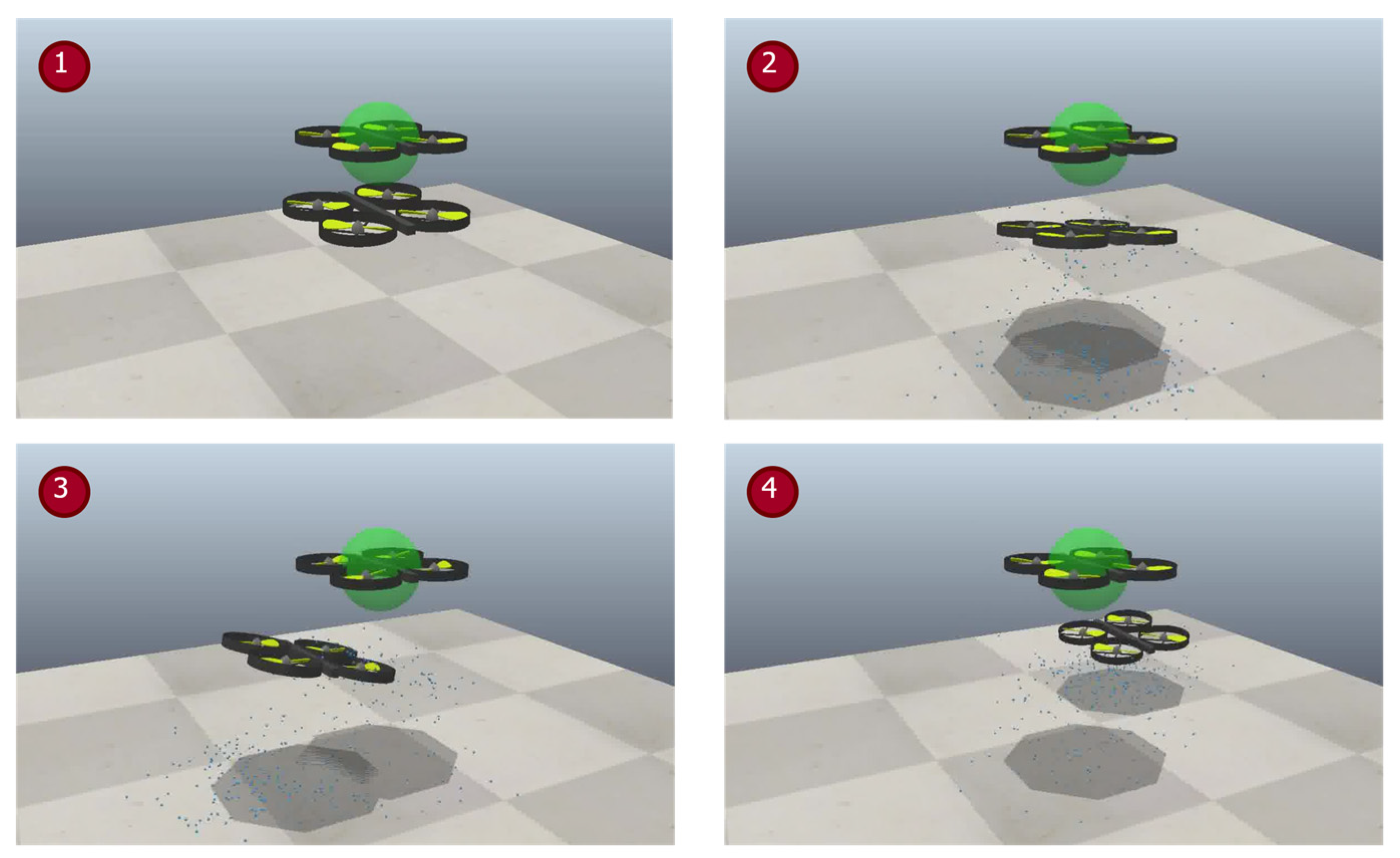
Aerospace 11 00237 g007
Figure 8. Procedurally generated terrain in 3D space for swarm navigation test.
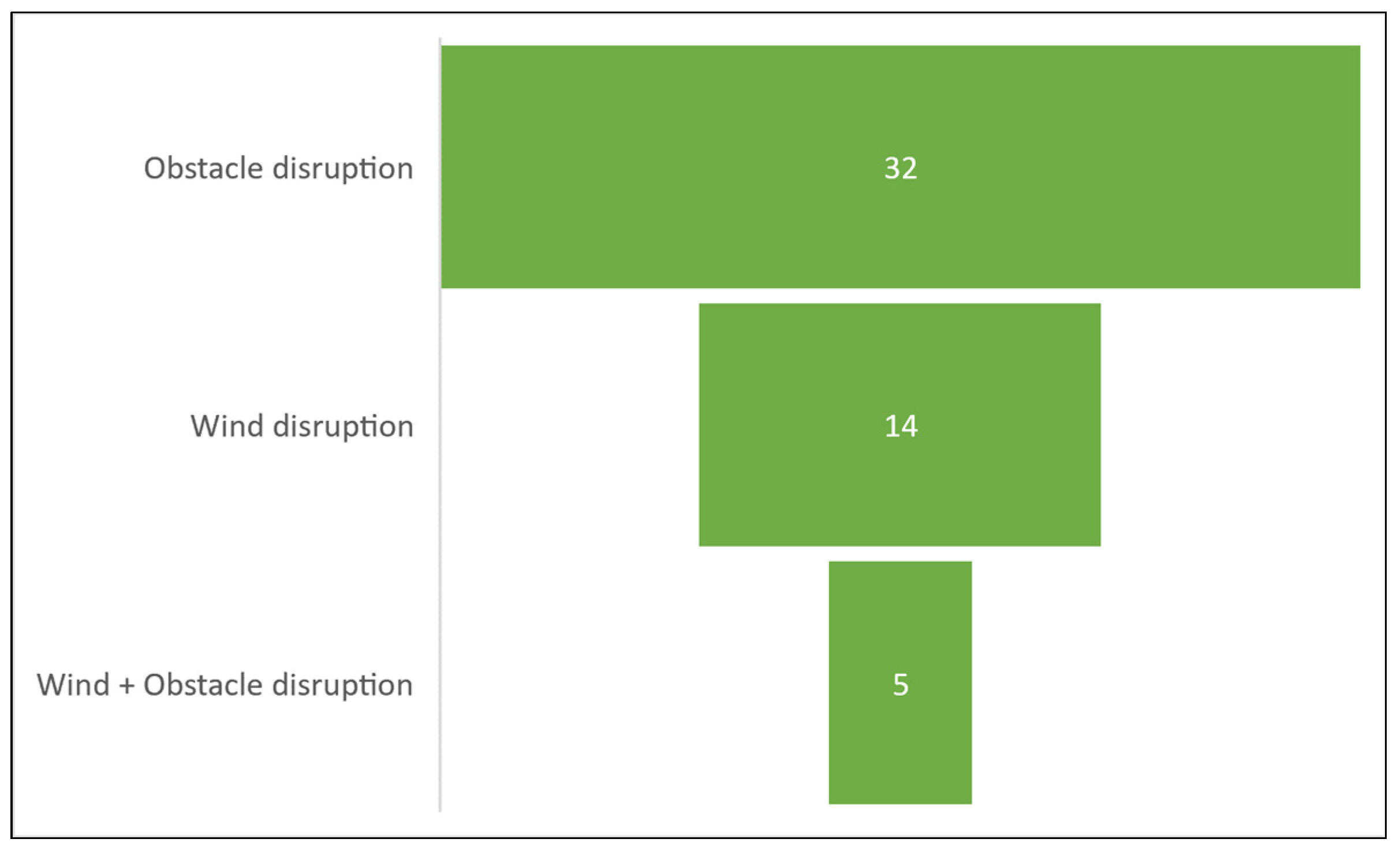
Aerospace 11 00237 g008
Figure 9. Relevant research examined in the bibliometric analysis in [26,27] that categorizes disturbance simulations into three categories.
Aerospace 11 00237 g009
Figure 10. Scenario 1.1: visually represents wind force modeling over a grid-based ROI.
Aerospace 11 00237 g010
Figure 11. Scenario 1.1: a 2D grid ROI with wind values and obstacles, showing a sample channel scenario.
Aerospace 11 00237 g011
Figure 12. Scenario 1.2: a 3D channel-based wind grid with different wind speeds.
Aerospace 11 00237 g012
Figure 13. Scenario 1.3: downwash drift occurrence near agents in 3D simulation.
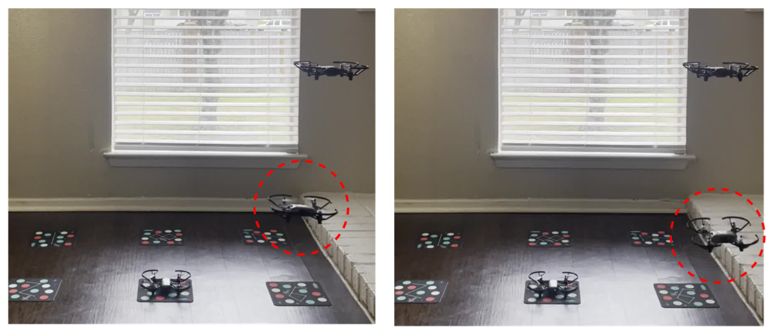
Aerospace 11 00237 g013
Figure 14. Downwash drift occurrence in agents in close proximity in the real world.
Aerospace 11 00237 g014
Figure 15. Scenario 2.1: five agents are moving in 3D space for maximum area coverage in the presence of multiple obstacles.
Aerospace 11 00237 g015
Figure 16. Scenario 2.2 is a 3D simulation map with Gielis cones for obstacles.
Aerospace 11 00237 g016
Figure 17. Scenario 2.3 is a top-down view of a 3D simulation environment with a varied number of obstacles.
Aerospace 11 00237 g017
Figure 18. Experiment 1: UAV paths in the presence of wind and obstacles.
Aerospace 11 00237 g018
Figure 19. Changes in trajectories when the same agents 1 and 2 are exposed to wind and obstacles.
Aerospace 11 00237 g019
Figure 20. Path and trajectory deviation in 2D for a single agent on a smaller scale position.
Aerospace 11 00237 g020
Figure 21. Scenario 1.2: planning using wind channels and agent placement.
Aerospace 11 00237 g021
Figure 22. Scenario 1.2 examines cohesion and agent performance using SwarmLab with wind constraints.
Aerospace 11 00237 g022
Figure 23. Experiment 2 using Scenario 2.2: the path traveled by a single agent in turbulence and no-turbulence scenarios (five iterations).
Aerospace 11 00237 g023
Figure 24. Experiment 2, Scenario 2.2: energy expenditure for the above agent for each iteration and average energy consumed over the total number of iterations.
Aerospace 11 00237 g024
Figure 25. Experiment 2, Scenario 2.2: paths traveled by five agents in turbulence and no turbulence scenario (one iteration).
Aerospace 11 00237 g025
Figure 26. Experiment 2, Scenario 2.2: energy expenditure for each agent for the single iteration in turbulence and no-turbulence scenario.
Aerospace 11 00237 g026
Figure 27. Experiment 3, Scenario 1.3: path deviation measured for lower UAV agent due to downwash from the upper agent.
Aerospace 11 00237 g027
Figure 28. Experiment 3, Scenario 1.3: the number of collisions during swarm movement when drift effects are considered.
Aerospace 11 00237 g028
Figure 29. Scenario 2.1: the relationship between area coverage by agent and probability of obstacle being present at next generated point.
Aerospace 11 00237 g029
Figure 30. A variation of Experiment 5 that has implemented Scenario 2.2 only: agents are moving in 3D environments populated with sparse complex obstacles.
Aerospace 11 00237 g030
Figure 31. Fragmentation phenomenon observed in simulations with concave surfaces over those with simpler obstacle geometry.
Aerospace 11 00237 g031
Figure 32. Change in swarm cohesion values for various case scenarios in Experiment 5.2.
Aerospace 11 00237 g032
Figure 33. Experiment 6: a dispersion action being tested for a three-vehicle swarm.
Aerospace 11 00237 g033
Figure 34. Sectional scene viewpoint and multiple camera feeds of the agents moving in the simulated space.
Aerospace 11 00237 g034
Figure 35. Experiment 6 result plot showcasing the encounter rates of varied obstacles for a three-agent swarm over 25 experiment iterations.
Aerospace 11 00237 g035
Figure 36. A UAV block diagram focusing on motor dynamics and a variable number of motors.
Aerospace 11 00237 g036
Figure 37. A fault injection and observation process framework for a UAV in a simulation environment.
Aerospace 11 00237 g037
Figure 38. An incident record of a faulty rotor during an RPM pose check before the agent takes off.
Aerospace 11 00237 g038
Figure 39. The sequence of UAV landing events after a simulation of a rotor failing.
Aerospace 11 00237 g039
Figure 40. A general process for simulation of network disturbances.
Aerospace 11 00237 g040
Figure 41. OMNET++ implementation of mobile ROI and intrusion detection mission using five agents.
Aerospace 11 00237 g041
Figure 42. Experiment results for ROI and intrusion detection study conducted in line with the proposed disruption methodology in Figure 40.
Aerospace 11 00237 g042
Figure 43. Heatmap of intrusion records for the above conducted experiments.
Aerospace 11 00237 g043
Table 1. Relevant research incorporating wind models in swarm simulations.
ReferenceDescription
[17]Studies the effect of wind on the connectivity and safety of a large-scale swarm.
[16]Analyze the impacts of wind speed, direction, and turbulence on sUAS (Small Unoccupied Aircraft System).
[18]Novel APF-based path planning technique for following GMTs (Ground Moving Targets) in a windy environment.
[19]Cooperative tracking for fixed-wing UAVs in the presence of an unknown wind component.
[20]Method to accurately estimate and compensate for wind gusts, acting on the nonlinear quadrotor in real-time.
[15]Mechanism of UAV movement in the wind field from velocity, force, and energy viewpoint.
Table 2. Relevant research incorporating obstacle models in swarm simulations.
ReferenceDescription
[28]Formation control and link selection for UAVs in complex environments using APF.
[29]Method for UAV avoiding dynamic obstacles using their velocity as input in a noisy environment.
[30]Reinforcement-learning-based method for UAVs to avoid obstacles in variable map sizes and swarm sizes.
[31]A dual-based flocking obstacle avoidance algorithm for dealing with narrow obstacles.
[32]Obstacle and collision avoidance for UAV swarm based on vector field histogram algorithm.
[33]Improved APF method that can plan a smooth, reasonable path with reduced energy consumption.
[34]A hierarchical weighting Vicsek model for swarm alignment and obstacle avoidance.
Table 3. Relevant research incorporating both obstacles and wind disturbance.
ReferenceDescription
[35]Local obstacle avoidance control scheme for UAV with suspended payload for complex environments with dense obstacles and wind.
[36]Obstacle avoidance for fixed-wing aircraft in no-fly zones in the presence of wind disturbances.
[37]Energy-efficient UAV mission planning in the presence of wind was simulated using the Dryden turbulence model.
[38]Bio-inspired swarm control under dynamic obstacle interference.
Table 4. Wind disruption scenario design with experiment process for disruption modeling and use-case scenario.
Scenario NumberScenario DesignScenario Suitability
Scenario 1.1Region of interest (ROI) is divided into cells with a wind speed value.Incorporate current 2D simulations for path planning and obstacle avoidance where wind effects are not considered.
Scenario 1.2A 3D wind channel design with different wind speeds and directions.Suitable for 3D simulation environments where the above implementations are observed along with factors such as swarm cohesion changes in wind effects with altitude.
Scenario 1.3Close contact agents are showing drift and movement due to downwash.Suitable for swarm implementations where downwash and induced airflow effects of agents are not considered.
Table 5. Ostacle scenario design with experiment process for disruption modeling and use-case scenario.
Scenario NumberScenario DesignScenario Suitability
Scenario 2.1Grid-based modelsIncorporate in basic 2D and 3D environments to test the feasibility of obstacle avoidance, time to consensus, and swarm cohesion factors.
Scenario 2.2Complex geometry in sparse 3D environmentsIncorporate in 3D environments to extend obstacle property beyond simplified geometric shapes.
Scenario 2.3Simulator-supported 3D modelingIncorporate simulation platforms where obstacle property is given primary focus to study how different obstacles influence agent and swarm performance.
Table 6. Types of obstacles designed in the simulated environment and their characteristics.
Obstacle NameCharacteristic
Bird Dynamic, fast, small
BusDynamic, slow, large
CarDynamic, fast, large
Pedestrian Dynamic, slow, small
BuildingStatic, very large
TreeStatic, small
Table 7. A summary of created scenarios characterized by their major disruption, minor disruption (if any), and the dimensionality of the induced disruption.
Scenario NumberMajor DisruptionMinor DisruptionNature of Major Disruption
1.1WindObstacles2D
1.2WindObstacles3D
1.3WindNA3D
2.1ObstaclesNA3D
2.2ObstaclesWind3D
2.3ObstaclesNA3D
Table 8. Scenario numbers are categorized by the type of UAV swarm agents used and their connection scheme.
Scenario NumberAgent Properties
1.1Point mass UAV agents connected in a decentralized manner
1.2Point mass UAV agents connected in a decentralized manner
1.33D models of UAV agents with no defined inter-agent connection
2.1Point mass UAV agents connected via a sparse agent-aware connection
2.2Point mass UAV agents connected in a centralized leader–follower strategy
2.33D models of UAV agents via sparse agent-aware connection
Table 9. Wind disruption experiment objectives and the scenarios they use for wind disruption analysis.
Experiment NumberScenario UsedObjective
1Scenario 1.1Test changes in trajectory deviation for agents deployed in Scenario 1.1.
2Scenario 1.2Incorporate the designed 3D wind grid with agents to measure energy changes consumed in the presence of wind factors.
3Scenario 1.3Observe agent interactions due to induced airflow in proximity.
Table 10. Obstacle disruption experiment objectives and the scenarios they use for wind disruption analysis.
Experiment NumberScenario UsedObjective
4Scenario 2.1Test changes in area coverage when a swarm is subjected to dense obstacles.
5Scenario 1.2 and 2.2Test swarm cohesion metric in the presence of wind and obstacles (two experiment variations: Experiment 5.1 with only Scenario 2.2; and Experiment 5.2 with Scenarios 1.2 and 2.2 implemented).
6Scenario 2.3Record the variability and encounter rate allowed by Scenario 2.3 in swarm agent deployment.
Table 11. A summary of the experiment numbers and the major disruption effects observed.
Experiment NumberMajor Effect of Disruption Observed
1Demonstrate changes in path and trajectory based on the introduction of obstacles and wind.
2Demonstrate changes in agent energy consumption as UAV moves in the absence and presence of turbulence.
3Demonstrate the effect of induced airflow and downwash on agents near each other in terms of collision occurrence.
4Demonstrate changes in vital swarm functions such as area coverage in the presence of obstacles.
5Demonstrate changes in a vital metric: swarm cohesion as agents move in the disruption scenario.
6Demonstrate the result of effective disruption modeling when agents encounter variable obstacles in the modeled scenario.
Disclaimer/Publisher’s Note: The statements, opinions and data contained in all publications are solely those of the individual author(s) and contributor(s) and not of MDPI and/or the editor(s). MDPI and/or the editor(s) disclaim responsibility for any injury to people or property resulting from any ideas, methods, instructions or products referred to in the content.

