Seasonal Variations in Lunar-Assisted GEO Transfer Capability for Southward Launch

Abstract

The launch azimuth of the Naro Space Center is limited toward the south of the Korean peninsula, at 170 ± 10 degrees, suitable for the polar orbit, sun-synchronous orbit, and safety range issues. In this circumstance, one option to send a satellite into GEO is to perform a dog-leg maneuver during ascent, thus forming a medium-inclination orbit under such a restrictive condition. However, this option requires an immense amount of energy for the dog-leg maneuver, as well as a plane change maneuver. The only remaining option is to raise the apogee to the Moon, utilizing lunar gravity to lower the inclination to near zero and then returning to the vicinity of the Earth at an altitude of 35,786 km without maneuver. In order to design lunar-assisted GEO transfer, all feasible paths are defined, but questions remain about how seasonal variations affect all these potential paths. Therefore, this study aims to design and analyze all available trajectories for the year 2031 using a high-fidelity dynamic model, root-finding algorithm, and well-arranged initial conditions, focusing on the impact of seasonal trends. The simulation results indicate that cislunar free-return trajectories generally require less $\mathit{\Delta }V$ compared to circumlunar free-return trajectories, and circumlunar trajectories are minimally affected by lunisolar effects due to their relatively short return time of flight. Conversely, cislunar trajectories show seasonal variations, so spring and fall seasons require up to 20 m/s less $\mathit{\Delta }V$ than summer and winter seasons due to the relatively long time of return duration.

1. Introduction

Normally, it is preferred to have the launch site near the equator for a GEO satellite, and then it is also necessary to have as low an inclination as possible to minimize the plane change maneuver. However, Naro Space Center (NSC) is located at a northern latitude of 34° and launches should be performed southward, because it passes through Japanese territory if an eastward launch occurs. For this reason, the launch azimuth of the NSC is near 170°, and then the initial inclination of the satellite is approximately 80° [1]. Most of all, traditionally, it seems that it is not possible to launch a GEO satellite from NSC, so alternative ways need to be provided. One way is to perform a dog-leg maneuver of the launch vehicle during ascent. The dog-leg maneuver, also called yaw ascent, occurs when the launch vehicle is launched along a predefined azimuth and then performs a maneuver in the left or right direction during ascent to change the plane of the Earth orbit [2]. As there is an additional direction maneuver during ascent, this approach results in being less efficient than general ascent without a dog-leg maneuver and, finally, in less spacecraft mass capability on the initial parkin orbit. Although this approach forms a medium-inclination orbit, for example, a 40° inclination (from 80°), it still remains a big plane change maneuver. Therefore, this approach has continued difficulty when selecting it. The practical final option is to utilize the Moon’s gravity to decrease the inclination to near zero without maneuvers and subsequently return to Earth, adjusting the trajectory to an altitude of 35,786 km in GEO to solve this problem.

Ivashkin et al. first showed a stationary Earth-satellite orbit injection using the Moon’s gravitational field [3]. Graziani et al. also provided a concept of GEO transfer from a launch site at a high latitude using the gravitational field of the Moon and found that Lunar Gravity Assist (LGA) is more efficient if the initial inclination is higher than 25.9° [4]. Circi et al. recognized that lunar-assisted transfers have an economical trajectory if the initial inclination is greater than the inclination of the Moon and provided results for a few different times of the year [5]. Ocampo provided an approximate model for the motion in the Earth–Moon system using a restricted three-body problem and rescue mission via LGA for AsisSat-3, which was successfully achieved in spite of the failure of the last stage of the launch vehicle [6,7]. Ramanan et al. also performed a GEO transfer using a genetic algorithm with adaptive bounds to avoid the sensitivity problem due to the initial conditions [8]. Previous research utilized only a subset of possible paths, and this field has seen limited study. For this reason, Choi et al. conducted a comprehensive analysis by defining all possible paths and then systematically organized the relationships between the time of flight and required $∆\mathrm{V}$ [9]. In September 2021, Spaceflight Inc. announced that a rideshare mission of “GEO Pathfinder” will be launching on a SpaceX Falcon 9 in 2024 with the main payload of a lunar lander mission (IM-2 Lunar Lander). An orbital transfer vehicle named “Sherpa-EA” delivers the GEO satellite after separation from cislunar orbit to GEO using an LGA scheme [10]. In order to make a good initial guess, Short et al. used a mapping-based approach for the Circular-Restricted Three-Body Problem, Bicircular Four-Body problem. and Moon–Earth–Sun problem [11]. Furthermore, Bakhtiari et al. introduced a simultaneous orbit and attitude initial states correction algorithm to achieve precise initial conditions [12].

There are various possible paths, consisting of two free-return trajectories, two nodes (descending and ascending) of the Moon’s orbit, and two departure trajectories. The most important factor in designing the trajectory using LGA is to use the free-return trajectories (circumlunar and cislunar). The cislunar free-return trajectory is where the apogee and perilune at the lunar flyby are located in the line between the Earth and Moon, whereas the circumlunar free-return trajectory is where the apogee and perilune are located out of the line between the Earth and Moon [13]. Therefore, the apogee altitude for circumlunar free return is higher than that for cislunar free return. Another important factor is the flyby time, when the Moon passes through the near ascending and descending node of the equator of the Earth. An ascending node of the Moon’s orbit means that the Moon crosses the equator from south to north and a descending node of the Moon’s orbit means the Moon crosses the equator from north to south. Only these times provide a chance to have a near-zero inclination of the GEO satellite. Ascending and descending nodes of the Moon’s orbit occur every sidereal period of the Moon with respect to the Earth, and the time difference between them is approximately 14 days. The other important factor is the departure geometry affected by the launch environment and facility readiness. Ascending departure refers to the trajectory where the satellite passes over the Earth’s North Pole and travels towards the Moon, while descending departure refers to the trajectory where the satellite passes over the Earth’s South Pole [14].

Although Choi et al. showed best path for $∆\mathrm{V}$ among all possible paths [9], curiosity about how all these paths are influenced by the time, namely, the seasonal trend, still remains. Therefore, the goal of this work was to design all available trajectories based on the year 2031 and analyze how seasonal variations affect performance. The simulation results comprehensively figured out that cislunar free return tended to have less $∆\mathrm{V}$ than circumlunar free return, and the circumlunar trajectories were not influenced by the lunisolar effect, because the time of flight (3−4 days) of return trajectories is relatively short. On the other hand, cislunar free-return trajectories showed that the spring and fall seasons required $∆\mathrm{V}$ of up to 20 m/s less than the summer and winter seasons, which is because lunisolar perturbation affects long return trajectories (13−17 days). This study demonstrated that an economical choice is possible by presenting the distribution of $∆\mathrm{V}$ concerning seasonal variations when utilizing related trajectories. Additionally, it provided a fundamental alternative by allowing a satellite with a high initial inclination to reach GEO.

Section 2 defines all available paths based on the Earth departure, node of the Moon’s orbit, and free-return trajectories. It explains the differentiation between circumlunar and cislunar return by defining the values of the B-plane parameters. Additionally, by predicting the Moon’s right ascension, declination, and time using JPL DE421 ephemeris, it outlines the necessary conditions for the right ascension of the ascending node (RAAN) and argument of perigee (AOP) needed to design LGA. Section 3 describes a four-body dynamic model and numerical search method, as well as the initial conditions for mission scenarios. Section 4 shows the simulation results, their trajectories in terms of free-return trajectories, and a coordinate system such as for Earth inertial and Earth–Moon rotating. Converging parameters such as the initial RAAN, AOP, $B_t$, and $B_r$ for all possible paths and seasonal variations for $\mathit{\Delta }V$ and $\mathit{\Delta }t$ are depicted in detail. Finally, Section 5 summarizes the overall conclusions.

2. Problem Description

2.1. Possible Paths

Using lunar gravity assist to shift the high inclined orbit to near zero, the lunar flyby should occur at a node of the Moon’s orbit [3,4,9]. There are two nodes of the Moon, where one is the ascending node of the Moon and the other is the descending node of the Moon with respect to the equator of the Earth. The occurrence times of the two nodes repeating every lunar month in 2031 can be easily calculated using JPL DE421 ephemeris. As shown in Figure 1, “circumlunar” refers to it occurring at the perilune on the far side of the Moon, and “cislunar” refers to it occurring at the perilune on the near side of the Moon [13].

In this situation, the circumlunar return trajectory has a short time of flight (TOF) of about 3.5 days, while the cislunar return trajectory has a long TOF of about 12 to 23 days. One remaining option is the departure trajectory when transferring to the Moon, where ascending departure refers to passing over the Earth’s North Pole, while descending departure refers to passing over the Earth’s South Pole. Figure 1 shows four paths by using the two departures and two free-return trajectories with respect to the ascending node of the Moon’s orbit, and four other paths are possible with respect to the descending node of the Moon’s orbit. With the combination of the departure, the node of the Moon’s orbit, and the free-return trajectory, abbreviations for the eight possible paths are defined by AACCL (ascending departure, ascending node of Moon’s orbit, and CirCumLunar), ADCCL, DACCL, and DDCCL for circumlunar free-return trajectories and AACSL, ADCSL, DACSL, and DDCSL for cislunar free-return trajectories. Most of the previous studies have focused on circumlunar free returns [4,6,7,8], and Circi et al. studied both types of free return [5], while Choi et al. performed all possible paths and figured out that ADCSL requires a minimum ΔV among the paths [9].

2.2. B-Plane

B−Plane parameters, which are defined in a polar coordinate system of an assisting body or other celestial body, have been widely used for targeting problems in gravity assist and interplanetary missions [15]. The coordinate system used for the B−plane is based on the Lunar Mean Equator and International Astronomical Unit vector of J2000, with the k-vector pointing toward the north pole of the Moon. The lunar B−plane, which consists of $B_r$ and $B_t$, is a mathematical construct that lies perpendicular to the incoming asymptote of hyperbola and provides a convenient set of linear targets for a spacecraft approaching the Moon, as described in Figure 2 [16]. The positive direction of $B_t$ is “rightward” and the positive direction of $B_r$ is “downward”. As the B−plane is easy to use as a constraint in numerical search algorithms, its components are used as coarse pointing parameters to design LGA.

The targeted B−plane values for lunar flyby are carefully selected to approach the satellite on the near side of the Moon (cislunar free return) and far side of the Moon (circumlunar free return). For example, a negative value of $B_t$ is required for a circumlunar free-return trajectory, while a positive value of $B_t$ is required for a cislunar free-return trajectory. In the case of $B_r$, a near-zero value is assumed as an initial condition.

2.3. Moon’s Position and Necessary Condition for LGA

The lunar sidereal period with respect to the Earth is around 27.3 days, so based on observing four lunar cycles from 1 November 2030 to 1 March 2031, the distance of the Moon’s orbit is estimated to be between 355,000 km and 405,000 km, as described in Figure 3a. The declination of the moon (${\delta }_{Moon}$) shows a similar pattern to the distance of the Moon. The ascending node (▲) and the descending node (▼) occur once per lunar cycle, with an interval of approximately 13.7 days between the two nodes. The direct lunar flyby is established through a minimum energy ellipse with a perigee radius and the apogee radius at the lunar distance that involves maneuvering in the direction of the velocity vector at the perigee of the parking orbit. To target a lunar encounter at apogee, there is the necessary condition that the apogee radius vector should lie in the plane of the Moon’s orbit, which requires a unique combination for RAAN and AOP [7]. In addition, flyby should occur at the ascending or descending node of the Moon’s orbit.

Once we know the accurate time when the node of the Moon’s orbit occurs, the Earth departure epoch of a satellite can be easily calculated based on the TOF from the Earth to the Moon, and the initial condition of AOP (${\omega }_0$) is zero or 180° because the Moon is located at the near equator at the time of flyby. The right ascension of the Moon (${\alpha }_{Moon}$) at the time of the ascending and descending node of the Moon is approximately 347° and 167°, respectively, according to Figure 3b, and the difference between them is around 180°. This provides us with crucial information that the initial condition of the RAAN (${\mathsf{\Omega }}_0$) is highly correlated with the ${\alpha }_{Moon}$ at the lunar flyby, and thus, ${\mathsf{\Omega }}_0$ is 167° or 347°, depending on the geometry of the Earth departure and node of the Moon. In summary, by predicting the Moon’s right ascension and declination at the time of the node, the necessary conditions of the RAAN, AOP, and departure time of a GEO satellite can be outlined to design LGA.

3. Dynamic Model and Numerical Search Method

3.1. Dynamic and Propagation Model

The equations of motion in this problem can be written as follows [17]: the first term of Equation (1) describes Newton’s formulation of the gravitation of two orbiting bodies, the second term describes the third-body gravitational perturbation, the third term represents other forces affecting the GEO spacecraft, and the fourth term means thrust force using an on-board propulsion system [17]:

$$\ddot{\mathbf{r}}=-\mu \frac{\mathbf{r}}{{‖\mathbf{r}‖}^3}+\sum _{i>0}{\mu }_i\left(\frac{{\mathbf{r}}_{Bi}-\mathbf{r}}{{‖{\mathbf{r}}_{Bi}-\mathbf{r}‖}^3}-\frac{{\mathbf{r}}_{Bi}}{{‖{\mathbf{r}}_{Bi}‖}^3}\right)+\frac{1}{m}{\mathbf{F}}_s+\frac{1}{m}{\mathbf{F}}_T$$

(1)

where $\ddot{\mathbf{r}}$ and $\mathbf{r}$ are the acceleration and position of the spacecraft relative to a coordinate system with an origin $B_0$. The gravitational parameters for $B_0$ (reference gravitational body) and $B_i$ (i–th gravitational body) are $\mu$ and ${\mu }_i$. The position of $B_i$ relative to $B_0$ is ${\mathbf{r}}_{Bi}$. This problem deals with multiple bodies; for example, if the spacecraft is orbiting the Earth, the reference central body is the Earth ($\mu$ is Earth), while the Sun and the Moon are modeled as particle masses (${\mu }_i$ are Sun and Moon) to integrate Equation (1). On the other hand, if the spacecraft is within the sphere of influence (SOI) of the Moon, $\mu$ should use the Moon’s gravitational parameters and ${\mu }_i$ should be the Sun and Earth, as described in

Table 1. Propagation models for Earth and Moon.

Model	Earth Propagator	Moon Propagator
Gravitational field ($\mu$)	WGS84–EGM96 21 × 21	LP150Q 48 × 48
Atmospheric drag	Jacchia–Roberts	–
Solar radiation pressure	Dual cone	Dual cone
Third bodies (${\mu }_i$)	Sun, Moon	Earth, Sun
SOI distance	925,000 km	66,185 km

. The mass of the spacecraft is $m$, ${\mathbf{F}}_s$ consists of atmospheric drag and the solar radiation pressure (SRP) force, and ${\mathbf{F}}_T$ is the thrust force using an on-board propulsion system. Atmospheric drag is modeled if the spacecraft is within a low altitude of the Earth. The drag coefficient is assumed to be 2.2 and the SRP is generated by the radiation from the Sun within the solar system, so the SRP coefficient to simulate the effect of the SRP on the spacecraft is assumed to be 1.0. The cross-sectional area is assumed to be 4 m² and the mass of the spacecraft is 500 kg.

For propagation, a seventh-order Runge–Kutta–Fehlberg integrator with an eighth-order error control and variable step size control was used. The integrator uses an absolute error tolerance of 1 × 10⁻¹⁰ and a relative error tolerance of 1 × 10⁻¹³.

3.2. Mission Scenario and Initial Conditions (I.Cs)

The initial parking orbit of a GEO satellite launched from NSC has an altitude of 300 km and an inclination of 80° for a southward launch caused by safety range issues. The fixed orbital elements of the parking orbit are $a_0=6678$km$,$ $e_0=0.0,\mathrm{a}\mathrm{n}\mathrm{d}{i}_0=80°$ and remaining elements which are regarded as independent variables are ${\mathsf{\Omega }}_0 \mathrm{a}\mathrm{n}\mathrm{d}{\omega }_0$ at the given time $t_0$, while ${\nu }_0=0,$ because the Trans Lunar Injection (TLI) would be performed at perigee.

An impulsive maneuver (${\mathit{\Delta }V}_0$) is performed to go to the periapsis of the Moon at a given time $t_0,$ as described in Figure 4, while it is possible to determine $t_0$ by choosing ${\mathit{\Delta }t}_1,$ which is the duration between $t_{\mathrm{l}\mathrm{g}\mathrm{a}}$ and $t_0$ described in (3), because we know when the Moon passes over the ascending node of the Moon’s orbit. If LGA changes the initial inclination to near zero, as well as the perigee altitude of the return trajectory to 35,786 km, another impulsive maneuver (${\mathit{\Delta }V}_1$) is performed to put the satellite into GEO at a given time $t_1$. Therefore, the total maneuvers can be described in (2) and the free-return TOF (${\mathit{\Delta }t}_2$), which is the duration between $t_1$ and $t_{\mathrm{l}\mathrm{g}\mathrm{a}}$, as described in (4).

$${\mathit{\Delta }V}_{Total}={\mathit{\Delta }V}_0+{\mathit{\Delta }V}_1$$

(2)

$${\mathit{\Delta }t}_1=t_{\mathrm{l}\mathrm{g}\mathrm{a}}-t_0$$

(3)

$${\mathit{\Delta }t}_2={t_1-t}_{\mathrm{l}\mathrm{g}\mathrm{a}}$$

(4)

After reviewing previous research, it was found that ${\mathit{\Delta }t}_1$ depended on ${\mathit{\Delta }V}_0$ and the range of this value was from approximately 4 to 6 days [9,14,18]. Therefore, ${\mathit{\Delta }t}_1$ is set to 5 days as an initial guess, and thus, $t_0=t_{\mathrm{l}\mathrm{g}\mathrm{a}}$ − 5 days and $t_{\mathrm{l}\mathrm{g}\mathrm{a}}$ is the time of the ascending or descending node of the Moon’s orbit. As mentioned in Section 2.3, a necessary condition requires a unique combination of the ${\mathsf{\Omega }}_0$ and ${\omega }_0$, while these combinations depend on the geometry between the Earth departure and node of the Moon. For ${\omega }_0$, ascending departure requires a near-zero degree because it will pass over the North Pole, but descending departure requires near 180°. For ${\mathsf{\Omega }}_0$, it is highly correlated with the right ascension of the Moon at flyby and it depends on both the Earth departure and node of the Moon. The ascending departure/ascending node of the Moon and descending departure/descending node of the Moon require ${\mathsf{\Omega }}_0=$ 167°, while the ascending departure/descending node of the Moon and descending departure/ascending node of the Moon require ${\mathsf{\Omega }}_0=$ 347°, regardless of the type of free-return trajectories. As a result, the initial conditions for four different combinations at $t_0$ are established in

Table 2. Initial conditions for four different combinations at given time $t_0$.

Type (Departure/Node)	${\mathbf{a}}_0$(km)	${\mathbf{e}}_0$	${\mathbf{i}}_0$(°)	${\mathsf{\Omega }}_0$(°)	${\mathsf{\omega }}_0$(°)	${\mathsf{\nu }}_0$(°)
Ascending/Ascending	6678	0.0	80.0	167	0.0	0.0
Ascending/Descending	6678	0.0	80.0	347	0.0	0.0
Descending/Ascending	6678	0.0	80.0	347	180.0	0.0
Descending/Descending	6678	0.0	80.0	167	180.0	0.0

.

$${\mathit{\Delta }V}_0=\sqrt[]{\frac{2\mu }{r_0}-\frac{\mu }{a_{lga}^{-}}}-\sqrt[]{\frac{\mu }{r_0}},{\mathit{\Delta }V}_1=\sqrt[]{\frac{\mu }{r_{\mathrm{f}}}}-\sqrt[]{\frac{2\mu }{r_{\mathrm{f}}}-\frac{\mu }{a_{lga}^{+}}}$$

(5)

Equation (5) describes the initial condition of ${\mathit{\Delta }V}_0$, where $a_{lga}^{-}$ means the semimajor axis from the Earth to Moon before a lunar flyby [19]. Using the mean Moon distance (384,400 km) at the node of the Moon’s orbit depicted in Figure 3a and $r_0$ (6678 km), the initial ${\mathit{\Delta }V}_0$ is guessed as 3106 m/s. In order to set the value of $a_{lga}^{+}$, it is necessary to first determine which free-return trajectory to use. According to the result of Choi et al. [9], $a_{lga}^{+}$ is around 600,000 km and 700,000 km for the circumlunar and cislunar free returns, respectively. Based on the $r_{\mathrm{f}}$ (42,164 km), the initial ${\mathit{\Delta }V}_1$ using Equation (5) for circumlunar and cislunar free returns are guessed as 1148 m/s and 1128 m/s.

3.3. Numerical Search Model

To design the trajectory of the GEO satellite using LGA, a differential corrections process using the Newton–Raphson method, which is a root-finding algorithm, was used [20]. This approach is a robust mathematical mechanism, and its form is described in Equation (6). The vector of the control variables is $\mathbf{x}$, the evaluation function using Equation (1) with a state vector of $\mathbf{x}$ is $\mathbf{f}\left(\mathbf{x}\right),$ and the vector of equality constraints is ${\mathbf{y}}_{\mathrm{d}}$ [20]:

$$\tilde{\mathbf{y}}=\mathbf{f}\left(\mathbf{x}\right)-{\mathbf{y}}_{\mathrm{d}}\approx 0$$

(6)

In order to solve Equation (6), a partial derivative of $\mathbf{f}\left(\mathbf{x}\right)$ is used with a Taylor series about the initial conditions of the control variables ${\mathbf{x}}_0$. A Jacobian matrix ($\mathbf{J}$) consisting of partial derivatives of $\mathbf{f}\left(\mathbf{x}\right)$ is described in Equation (7) [20] with the number of control variables ($\mathrm{n}$) and equality constraints ($\mathrm{m}$):

$$\mathbf{J}=\left[\begin{array}{ccc}\frac{{\partial }_{{\mathrm{y}}_1}}{{\partial }_{{\mathrm{x}}_1}}& \dots & \frac{{\partial }_{{\mathrm{y}}_1}}{{\partial }_{{\mathrm{x}}_{\mathrm{n}}}}\\ ⋮& \ddots & ⋮\\ \frac{{\partial }_{{\mathrm{y}}_{\mathrm{m}}}}{{\partial }_{{\mathrm{x}}_1}}& \dots & \frac{{\partial }_{{\mathrm{y}}_{\mathrm{m}}}}{{\partial }_{{\mathrm{x}}_{\mathrm{n}}}}\end{array}\right]$$

(7)

To find the control variable ($\mathbf{x}$) using a numerical search algorithm, Equation (6) can be rearranged as Equation (8) [20]. The i-th column of $\mathrm{J}$ is ${\mathbf{J}}_{\mathrm{i}}=(\mathbf{f}\left(\mathbf{x}+\mathsf{\delta }{\mathbf{x}}_{\mathrm{i}}\right)-\mathbf{f}\left(\mathbf{x}\right))/\mathsf{\delta }{\mathrm{x}}_{\mathrm{i}}$ and the perturbation of the i-th control variable is $\mathsf{\delta }{\mathbf{x}}_{\mathrm{i}}={\left[\begin{array}{cc}\begin{array}{cc}0& \dots \end{array}& \begin{array}{ccc}\mathsf{\delta }{\mathrm{x}}_{\mathrm{i}}& \dots & 0\end{array}\end{array}\right]}^{\mathrm{T}}$. This algorithm process repeats until the error of each equality constraint satisfies the predefined tolerance.

$${\mathbf{x}}_{\mathrm{k}+1}={\mathbf{x}}_{\mathrm{k}}-{\mathbf{J}}_{\mathbf{k}}^{-1}(\mathbf{f}\left({\mathbf{x}}_{\mathrm{k}}\right)-{\mathbf{y}}_{\mathrm{d}})$$

(8)

The trajectory design from LEO (Low Earth Orbit) to GEO using LGA is classified into two numerical search problems to enhance the convergence of the free-return trajectory after the flyby, where one is from LEO to the periapsis of the Moon and the other one is from LEO to GEO. The initial states are ${\mathbf{x}}_0=[{\mathrm{t}}_0,{\mathrm{a}}_0,{\mathrm{e}}_0,{\mathrm{i}}_0,{\mathsf{\Omega }}_0,{\mathsf{\omega }}_0,{\mathsf{\nu }}_0,{\mathit{\Delta }V}_0]$, while $[{\mathrm{a}}_0,{\mathrm{e}}_0,{\mathrm{i}}_0,{\mathsf{\nu }}_0]$ are already fixed, and thus, the remaining states are independent variables of ${\mathbf{x}}_0=[{\mathrm{t}}_0,{\mathsf{\Omega }}_0,{\mathsf{\omega }}_0,{\mathit{\Delta }V}_0]$ in Equation (8). The first part of the trajectory design is from LEO to perilune (${\mathrm{t}}_0\le \mathrm{t}\le {\mathrm{t}}_{\mathrm{l}\mathrm{g}\mathrm{a}}$) to distinguish the free-return trajectory, satisfying the equality constraints of ${\mathbf{y}}_{\mathrm{d}}=[{\mathrm{B}}_{\mathrm{t}},{\mathrm{B}}_{\mathrm{r}},{\mathit{\Delta }t}_1]$. For example, in the case of AACCL, where the ascending node of the Moon’s orbit is 29 December 2030 21:30:00 (UTC) shown in Figure 3b, the initial conditions are listed in Table 2 and the equality constraints are mentioned in Section 2.2, as described below.

The numerical search algorithm of the first part is rewritten in detail using independent variables and equality constraints with the tolerance vectors of $\tilde{\mathbf{y}}$ in Equation (9).

$${\mathbf{x}}_0={\left[\begin{array}{cccc}24 \mathrm{D}\mathrm{e}\mathrm{c}\mathrm{e}\mathrm{m}\mathrm{b}\mathrm{e}\mathrm{r} 2030 21:00:00& 167°& 0°& 3106 \mathrm{m}/\mathrm{s}\end{array}\right]}^{\mathrm{T}}$$

$${\mathbf{y}}_{\mathrm{d}}={\left[\begin{array}{ccc}-10000& 0.0& 5 \mathrm{d}\mathrm{a}\mathrm{y}\mathrm{s}\end{array}\right]}^{\mathrm{T}} \mathrm{f}\mathrm{o}\mathrm{r} \mathrm{c}\mathrm{i}\mathrm{r}\mathrm{c}\mathrm{u}\mathrm{m}\mathrm{l}\mathrm{u}\mathrm{n}\mathrm{a}\mathrm{r} \mathrm{f}\mathrm{r}\mathrm{e}\mathrm{e} \mathrm{r}\mathrm{e}\mathrm{t}\mathrm{u}\mathrm{r}\mathrm{n}$$

$${\mathbf{y}}_{\mathrm{d}}={\left[\begin{array}{ccc}10000& 0.0& 5 \mathrm{d}\mathrm{a}\mathrm{y}\mathrm{s}\end{array}\right]}^{\mathrm{T}} \mathrm{f}\mathrm{o}\mathrm{r} \mathrm{c}\mathrm{i}\mathrm{s}\mathrm{l}\mathrm{u}\mathrm{n}\mathrm{a}\mathrm{r} \mathrm{f}\mathrm{r}\mathrm{e}\mathrm{e} \mathrm{r}\mathrm{e}\mathrm{t}\mathrm{u}\mathrm{r}\mathrm{n}$$

$$\left[\begin{array}{c}{\mathrm{t}}_0^{\mathrm{n}\mathrm{e}\mathrm{w}}\\ {\mathsf{\Omega }}_0^{\mathrm{n}\mathrm{e}\mathrm{w}}\\ {\mathsf{\omega }}_0^{\mathrm{n}\mathrm{e}\mathrm{w}}\\ {\mathit{\Delta }V}_0^{\mathrm{n}\mathrm{e}\mathrm{w}}\end{array}\right]=\left[\begin{array}{c}{\mathrm{t}}_0^{\mathrm{o}\mathrm{l}\mathrm{d}}\\ {\mathsf{\Omega }}_0^{\mathrm{o}\mathrm{l}\mathrm{d}}\\ {\mathsf{\omega }}_0^{\mathrm{o}\mathrm{l}\mathrm{d}}\\ {\mathit{\Delta }V}_0^{\mathrm{o}\mathrm{l}\mathrm{d}}\end{array}\right]-{\mathbf{J}}_{\mathbf{k}}^{-1}\left(\mathbf{f}\left[\begin{array}{c}{\mathrm{t}}_0^{\mathrm{o}\mathrm{l}\mathrm{d}}\\ {\mathsf{\Omega }}_0^{\mathrm{o}\mathrm{l}\mathrm{d}}\\ {\mathsf{\omega }}_0^{\mathrm{o}\mathrm{l}\mathrm{d}}\\ {\mathit{\Delta }V}_0^{\mathrm{o}\mathrm{l}\mathrm{d}}\end{array}\right]-\left[\begin{array}{c}{\mathrm{B}}_{\mathrm{t}}\\ {\mathrm{B}}_{\mathrm{r}}\\ {\mathit{\Delta }t}_1\end{array}\right]\right),\tilde{\mathbf{y}}=\left[\begin{array}{c}{\mathrm{e}}_{{\mathrm{B}}_{\mathrm{t}}}\\ {\mathrm{e}}_{{\mathrm{B}}_{\mathrm{r}}}\\ {\mathrm{e}}_{{\mathit{\Delta }\mathrm{t}}_1}\end{array}\right]=\left[\begin{array}{c}1.0 \mathrm{k}\mathrm{m}\\ 1.0 \mathrm{k}\mathrm{m}\\ 10 \mathrm{s}\mathrm{e}\mathrm{c}\end{array}\right]$$

(9)

The first part aims to distinguish different types of free return, but in fact, a more crucial aspect is finding the initial conditions of the control variables to enhance the convergence of the free-return trajectories after flyby. Therefore, the converged control variables (${\mathbf{x}}_0^{\mathrm{n}\mathrm{e}\mathrm{w}}$) are used as the initial conditions for the second part (${\mathrm{t}}_0\le \mathrm{t}\le {\mathrm{t}}_1$), satisfying the equality constraints ${\mathbf{y}}_{\mathrm{d}}={[{\mathrm{r}}_{\mathrm{f}},{\mathrm{i}}_{\mathrm{f}},{\mathrm{V}}_{\alpha }]}^{\mathrm{T}}$ after flyby to reach GEO, where ${\mathrm{V}}_{\alpha }$ is the azimuth velocity. The numerical search algorithm of the second part is rewritten in detail using the converged independent variables (${\mathbf{x}}_0^{\mathrm{n}\mathrm{e}\mathrm{w}’}$) and equality constraints with the tolerance vectors ($\tilde{\mathbf{y}}$) in Equation (10).

$${\mathbf{x}}_0={\left[\begin{array}{cccc}{\mathrm{t}}_{0\_\mathrm{n}\mathrm{e}\mathrm{w}}& {\mathsf{\Omega }}_{0\_\mathrm{n}\mathrm{e}\mathrm{w}}& {\mathsf{\omega }}_{0\_\mathrm{n}\mathrm{e}\mathrm{w}}& {\mathit{\Delta }V}_{0\_\mathrm{n}\mathrm{e}\mathrm{w}}\end{array}\right]}^{\mathrm{T}}$$

$${\mathbf{y}}_{\mathrm{d}}={\left[\begin{array}{ccc}\mathrm{42,164} \mathrm{k}\mathrm{m}& 0.0°& 90.0°\end{array}\right]}^{\mathrm{T}}$$

$$\left[\begin{array}{c}{\mathrm{t}}_0^{\mathrm{n}\mathrm{e}\mathrm{w}’}\\ {\mathsf{\Omega }}_0^{\mathrm{n}\mathrm{e}\mathrm{w}’}\\ {\mathsf{\omega }}_0^{\mathrm{n}\mathrm{e}\mathrm{w}’}\\ {\mathit{\Delta }V}_0^{\mathrm{n}\mathrm{e}\mathrm{w}’}\end{array}\right]=\left[\begin{array}{c}{\mathrm{t}}_0^{\mathrm{n}\mathrm{e}\mathrm{w}}\\ {\mathsf{\Omega }}_0^{\mathrm{n}\mathrm{e}\mathrm{w}}\\ {\mathsf{\omega }}_0^{\mathrm{n}\mathrm{e}\mathrm{w}}\\ {\mathit{\Delta }V}_0^{\mathrm{n}\mathrm{e}\mathrm{w}}\end{array}\right]-{\mathrm{J}}_{\mathbf{k}}^{-1}\left(\mathbf{f}\left[\begin{array}{c}{\mathrm{t}}_0^{\mathrm{n}\mathrm{e}\mathrm{w}}\\ {\mathsf{\Omega }}_0^{\mathrm{n}\mathrm{e}\mathrm{w}}\\ {\mathsf{\omega }}_0^{\mathrm{n}\mathrm{e}\mathrm{w}}\\ {\mathit{\Delta }V}_0^{\mathrm{n}\mathrm{e}\mathrm{w}}\end{array}\right]-\left[\begin{array}{c}{\mathrm{r}}_{\mathrm{f}}\\ {\mathrm{i}}_{\mathrm{f}}\\ {\mathrm{V}}_{\alpha }\end{array}\right]\right),\tilde{\mathbf{y}}=\left[\begin{array}{c}{\mathrm{e}}_{{\mathrm{r}}_{\mathrm{f}}}\\ {\mathrm{e}}_{{\mathrm{i}}_{\mathrm{f}}}\\ {\mathrm{e}}_{{\mathrm{V}}_{\alpha }}\end{array}\right]=\left[\begin{array}{c}1.0 \mathrm{k}\mathrm{m}\\ 0.1°\\ 1.0°\end{array}\right]$$

(10)

Once the free-return trajectory approach to the perigee radius for GEO is formulated, one more numerical search algorithm is performed to reach GEO, with an independent variable of ${\mathrm{x}}_0=[{\mathit{\Delta }V}_1=1148\mathrm{m}/\mathrm{s}]$ for circumlunar free return or ${\mathrm{x}}_0=[{\mathit{\Delta }V}_1=1128\mathrm{m}/\mathrm{s}]$ for cislunar free return, equality constraints of ${\mathrm{y}}_{\mathrm{d}}=[{\mathrm{e}}_{\mathrm{f}}=0.0]$ and $\tilde{\mathrm{y}}=[{\mathrm{e}}_{\mathrm{e}}=0.001]$, and ${\mathrm{e}}_{\mathrm{f}}$ as the final eccentricity and ${\mathrm{e}}_{\mathrm{e}}$ as the eccentricity error.

4. Simulation Results

4.1. Trajectory Overview

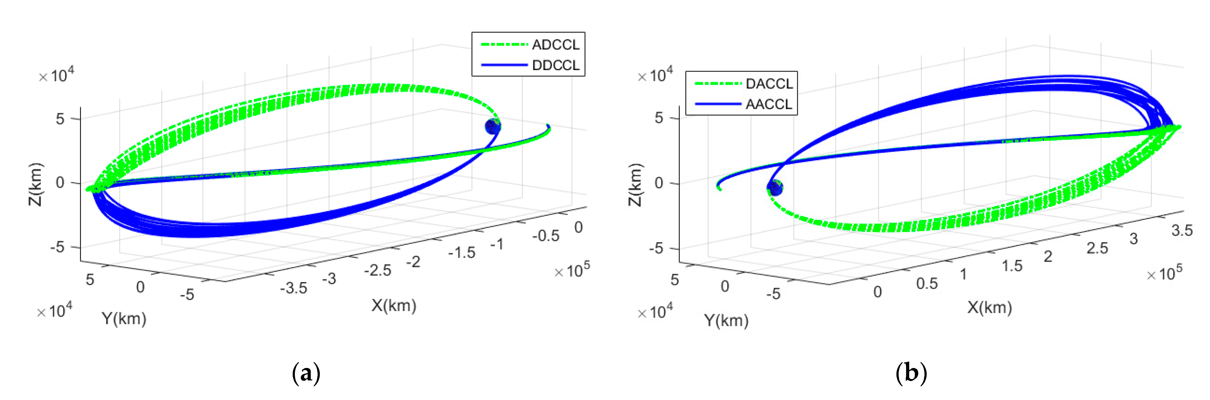
Figure 5 shows circumlunar free-return trajectories, where the apogee and perilune are located in the line between the Earth and Moon, for the target year of 2031 with respect to an Earth-Centered Inertial (ECI) frame and an Earth–Moon Rotating (EMR) frame. The ADCCL (green dotted line) and the DDCCL (blue solid line) used for the descending node of the Moon’s orbit and the DACCL (green dotted line) and the AACCL (blue solid line) used for the ascending node of the Moon’s orbit with respect to the ECI frame are shown in in Figure 5a,b, respectively. Although it has a high initial inclination, a near-zero inclination after flyby is available, and the free-return trajectories can be seen to have a similar pattern, regardless of which departure trajectory was used.

Figure 5c shows the circumlunar free-return trajectories with the descending node of the Moon’s orbit and Figure 5d shows the circumlunar free-return trajectories with the ascending node of the Moon’s orbit with respect to the EMR frame. When using the Moon’s descending node, the flyby distance from the Earth is approximately 400,000 km, whereas using the ascending node results in a flyby distance of about 380,000 km. Consequently, the required $\mathit{\Delta }{V}_0$(Trans–Lunar–Injection) using the descending node of the Moon’s orbit would be larger when using the ascending node of the Moon’s orbit.

Figure 6 shows cislunar free-return trajectories for the target year of 2031 with respect to an ECI frame and an EMR frame. The cislunar problem was solved using a numerical method; however, while ADCSL and DACSL could find continuous solutions on a monthly basis, DDCSL and AACSL could not find continuous solutions. Upon analyzing the process where solutions did not converge, it was observed that, after lunar flyby, either the ${\mathit{\Delta }t}_2$ became excessively large and did not converge, or even with an appropriate ${\mathit{\Delta }t}_2$, the GEO inclination did not converge to 0 degrees, but stayed below 5 degrees. This phenomenon occurred because the combination of the same Earth departure and the node of the Moon’s orbit (AA and DD) in a specific season created a geometry that was difficult to enter GEO due to the lunisolar effect. For DDCSL and AACSL, the seasonal convergence results are described in detail in

Table A1. Summary of converged results of DDCSL trajectories.

No.	${\mathit{t}}_0$(UTC)	${∆\mathit{V}}_0$(m/s)	${\mathit{t}}_{\mathbf{l}\mathbf{g}\mathbf{a}}$(UTC)	${∆\mathit{V}}_1$(m/s)	${\mathit{t}}_2$(UTC)	$∆\mathit{V}$(m/s)
1	2031-04-01 10:56:33	3104.73	2031-04-06 00:48:27	1128.24	2031-04-25 14:18:52	4232.97
2	2031-04-28 09:04:54	3105.50	2031-05-03 09:33:04	1119.24	2031-05-20 00:04:52	4224.74
3	2031-05-24 07:19:55	3111.06	2031-05-30 17:36:16	1127.16	2031-06-17 12:01:10	4238.22
4	2031-06-22 05:10:11	3107.85	2031-06-26 21:23:02	1133.16	2031-07-15 18:14:41	4241.01
5	2031-10-09 22:28:58	3106.66	2031-10-14 08:23:44	1128.13	2031-11-02 23:33:25	4234.79
6	2031-11-05 20:34:32	3106.75	2031-11-10 15:59:50	1119.80	2031-11-27 06:39:31	4226.55
7	2031-12-02 18:38:18	3108.42	2031-12-07 22:37:28	1124.91	2031-12-24 22:02:37	4233.33
8	2031-12-30 16:35:13	3110.13	2032-01-04 02:05:38	1142.91	2032-01-25 10:59:48	4253.04

and

Table A2. Summary of converged results of AACSL trajectories.

No.	${\mathit{t}}_0$(UTC)	${∆\mathit{V}}_0$(m/s)	${\mathit{t}}_{\mathbf{l}\mathbf{g}\mathbf{a}}$(UTC)	${∆\mathit{V}}_1$(m/s)	${\mathit{t}}_2$(UTC)	$∆\mathit{V}$
1	2031-04-14 09:34:40	3105.04	2031-04-19 04:37:12	1137.45	2031-05-11 08:33:31	4242.50
2	2031-05-11 07:52:28	3105.51	2031-05-16 07:32:05	1134.80	2031-06-05 14:15:37	4240.31
3	2031-06-07 05:43:38	3106.07	2031-06-12 09:43:42	1147.32	2031-07-05 05:14:03	4253.38
4	2031-10-22 21:02:37	3103.24	2031-10-27 12:35:10	1133.56	2031-11-17 12:47:03	4236.80
5	2031-11-18 19:05:01	3104.38	2031-11-23 15:42:32	1133.56	2031-12-13 05:57:33	4237.94
6	2031-12-15 17:09:26	3104.71	2031-12-20 18:01:28	1149.38	2032-01-13 00:00:40	4254.08

.

Figure 6a,b show the ADCSL and DACSL trajectories with respect to the ECI frame, and Figure 6c,d show the trajectories with respect to the EMR frame. In general, the DACSL trajectories appear more dispersed compared to the ADCSL trajectories. Specifically, from an EMR frame perspective, the departure trajectories of DACSL are slightly more convex than ADCSL, because the flyby distance from the Earth center of the ADCSL is slightly farther than the flyby distance of the DACSL. Furthermore, the free-return trajectories after a flyby of DACSL are more dispersed due to the increased influence of the lunar gravity compared to ADCSL.

4.2. Converged Geometry

The set of converging right ascensions of the ascending node (${\mathsf{\Omega }}_0$) and argument of perigee (${\mathsf{\omega }}_0$) were as below and are depicted in Figure 7a; for DDCSL and AACSL, only seasonally converging results are obtained.

• for AACCL, ${\mathsf{\Omega }}_0\in$ [170.5°, 172.5°], ${\mathsf{\omega }}_0\in$ [357.9°, 360.4°]
• for AACSL, ${\mathsf{\Omega }}_0\in$ [175.2°, 179.0°], ${\mathsf{\omega }}_0\in$ [355.6°, 356.6°]
• for DDCCL, ${\mathsf{\Omega }}_0\in$ [170.5°, 172.5°], ${\mathsf{\omega }}_0\in$ [178.3°, 180.9°]
• for DDCSL, ${\mathsf{\Omega }}_0\in$ [171.5°, 175.5°], ${\mathsf{\omega }}_0\in$ [174.6°, 180.5°]
• for ADCCL, ${\mathsf{\Omega }}_0\in$ [350.0°, 352.0°], ${\mathsf{\omega }}_0\in$ [1.0°, 3.6°]
• for ADCSL, ${\mathsf{\Omega }}_0\in$ [347.5°, 351.5°], ${\mathsf{\omega }}_0\in$ [0.0°, 3.1°]
• for DACCL, ${\mathsf{\Omega }}_0\in$ [349.5°, 351.2°], ${\mathsf{\omega }}_0\in$ [180.6°, 183.4°]
• for DACSL, ${\mathsf{\Omega }}_0\in$ [347.9°, 353.0°], ${\mathsf{\omega }}_0\in$ [180.0°, 182.7°]

As mentioned in the initial conditions specified in Table 2, ${\mathsf{\Omega }}_0$ for “AA” and “DD” was 167° and ${\mathsf{\Omega }}_0$ for “DA” and “AD” was 347°, while ${\mathsf{\omega }}_0$ for “AA” and “AD” was 0° and ${\mathsf{\omega }}_0$ for “DA” and “DD” was 180°. These results show that the initial conditions are a good starting point for the GEO transfer trajectory and the circumlunar free-return trajectories have a less dispersed set of ${\mathsf{\Omega }}_0$ and ${\mathsf{\omega }}_0$ compared to the cislunar free return.

All the circumlunar return trajectories have a negative ${\mathrm{B}}_{\mathrm{t}}$ value and its mean value of ${\mathrm{B}}_{\mathrm{r}}$ is near zero, while all the cislunar return trajectories have a positive ${\mathrm{B}}_{\mathrm{t}}$ value, as shown in Figure 7b. The “AA” and “DD” combination has a near-zero value of ${\mathrm{B}}_{\mathrm{r}},$ regardless of return trajectories, and the cislunar return trajectories of ${\mathrm{B}}_{\mathrm{r}}$ are more dispersed compared to the circumlunar return trajectories. The reason for this is that the cislunar free return for the combination of “AA” and “DD” only converging seasonally is thought to be the difficulty in sufficiently reducing the high initial inclination, as ${\mathrm{B}}_{\mathrm{r}}$ converges around zero. In contrast, cislunar trajectories with the “AD” and “DA” combination converge to a relatively large value of ${\mathrm{B}}_{\mathrm{r}}$, forming favorable geometries for reducing the high initial inclination.

4.3. ΔV and $\mathit{\Delta }t$

For the TLI $\mathit{\Delta }V$ shown at the top of Figure 8a, all TLI $\mathit{\Delta }V$s tended to have similar values (TLI $\mathit{\Delta }V\in$ [3100, 3115]), and cases that use the descending node of the Moon’s orbit (dotted line) require a little bit more $\mathit{\Delta }V$ than cases that use the ascending node of the Moon due to the flyby distance from the center of the Earth. On the other hand, GEO insertion $\mathit{\Delta }V$ at the bottom of Figure 8a demonstrates which combination requires the minimum amount of $\mathit{\Delta }V$ and how the $\mathit{\Delta }V$ varies depending on the seasonal influences. First, the circumlunar return trajectories were found to be minimally affected by seasonal factors, primarily influenced by both the Earth departure and node of the Moon. More importantly, DACCL consistently exhibited a low $\mathit{\Delta }V,$ regardless of the season, making it a favorable choice for the fast return trajectories. In contrast, the cislunar return trajectories demonstrated a low $\mathit{\Delta }V$ during spring and fall and a slightly higher $\mathit{\Delta }V$ during summer and winter, indicating a seasonal effect. This helped us to figured out that seasonal influence resulted in a maximum $\mathit{\Delta }V$ difference of approximately 20 m/s.

At the top of Figure 8b, the total $\mathit{\Delta }V$ shown is similar to the GEO insertion $\mathit{\Delta }V$, and it is observed that DDCCL without seasonal effects among the circumlunar return trajectories required the largest $\mathit{\Delta }V$ at around 4280 m/s, while the ADCSL needed the least $\mathit{\Delta }V$, reflecting seasonal influences effectively. According to a GEO transfer spacecraft launched from Cape Canaveral with an initial parking orbit (altitude of 185 km and an inclination of 28.5°), the total $\mathit{\Delta }V$ is around 4296 m/s, including $\mathit{\Delta }V$(2459 m/s) from LEO to GTO and $\mathit{\Delta }V$(1837 m/s) from GTO to GEO with a plane change maneuver [21]. The fact that a larger $\mathit{\Delta }V$ is required for a general GEO transfer with the most demanding DDCCL further validated the superiority of the method using LGA. Above all, this study numerically demonstrated that the cislunar return trajectories are influenced by seasonal variation. Additionally, it provided an alternative combination, defined as DACCL, that can be considered.

The bottom of Figure 8b illustrates the return TOF (${\mathit{\Delta }t}_2$) for both circumlunar and cislunar trajectories and its ranges were as below:

• for DDCCL, ${\mathit{\Delta }t}_1\in$ [4.31, 5.24], ${\mathit{\Delta }t}_2\in$ [2.80, 2.98]
• for DACCL, ${\mathit{\Delta }t}_1\in$ [4.31, 5.20], ${\mathit{\Delta }t}_2\in$ [3.08, 3.34]
• for ADCCL, ${\mathit{\Delta }t}_1\in$ [4.28, 5.35], ${\mathit{\Delta }t}_2\in$ [3.05, 3.25]
• for AACCL, ${\mathit{\Delta }t}_1\in$ [4.26, 5.20], ${\mathit{\Delta }t}_2\in$ [2.79, 3.01]
• for ADCSL, ${\mathit{\Delta }t}_1\in$ [4.22, 5.31], ${\mathit{\Delta }t}_2\in$ [11.55, 15.12]
• for DACSL, ${\mathit{\Delta }t}_1\in$ [3.97, 5.28], ${\mathit{\Delta }t}_2\in$ [13.38, 20.83]

The ${\mathit{\Delta }t}_2$ of the circumlunar return trajectories showed relatively short durations compared to ${\mathit{\Delta }t}_1$ and did not show seasonal variations, while the ${\mathit{\Delta }t}_2$ of the cislunar return trajectories was than 10 days. This easily leads to the conclusion that these cases reflect the seasonal factors related to the lunisolar effect. In addition, it was numerically confirmed that a shorter ${\mathit{\Delta }t}_2$ between ADCSL and DACSL results in a benefit in terms of $\mathit{\Delta }V$.

4.4. Analysis of Seasonal Factors

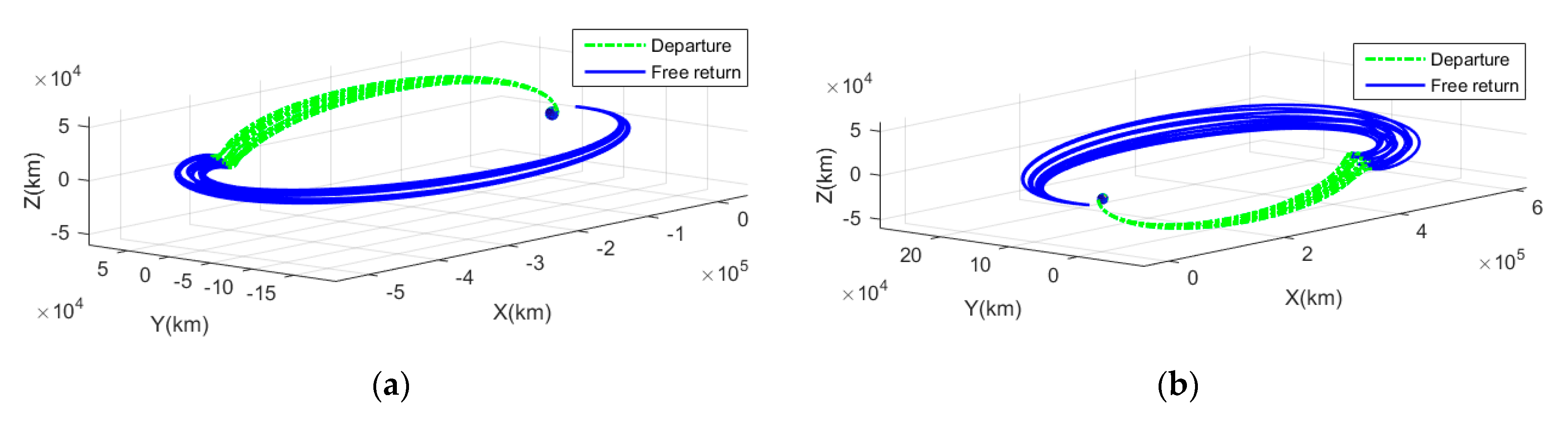
In order to specifically analyze the seasonal effect on the $\mathit{\Delta }V$, cislunar free-return cases were mapped in the Sun–Earth Rotating (SER) frame with the Earth, Sun, and Moon, as shown in Figure 9. The SER frame, also known as a heliocentric frame, was used to analyze the motion of objects in the solar system. In this frame of reference, the center of this frame is the Earth and the motion of the Earth and Sun appears stationary. The Moon is moving in its orbit around the center of the Earth, and thus, the Sun is located in the -X axis and the Z axis is perpendicular to the ecliptic plane.

Figure 9a,b show the thirteen trajectories of ADCSL and DACSL in 2031, respectively, which consist of departure (green dotted line) and free return (blue solid line). According to Figure 9, the Sun is located on the left side and the Moon rotates in the counterclockwise direction. As ${\mathit{\Delta }V}_1$ directly affects the $a_{lga}^{+}$ in Section 3.2, DACSL requires more ${\mathit{\Delta }V}_1$ than ADCSL to meet the near-zero eccentricity, because DACSL has a higher apogee altitude after flyby than ADCSL.

As illustrated in Figure 8b, the cislunar return trajectories exhibited a low $\mathit{\Delta }V$ during the late spring seasons (5,6,7) and late autumn seasons (12,13,14). Therefore, it was observed that it is advantageous for the position of apogee to be in either the second or fourth quadrant after flyby. Conversely, during the late winter seasons (2,3,4) and late summer seasons (8,9,10,11), the trajectory displayed a relatively higher $\mathit{\Delta }V$. Hence, it was noted that it is disadvantageous for the position of apogee to be in either the first or third quadrant after flyby.

5. Conclusions

This study designed a set of trajectories utilizing lunar gravity assist to avoid large plane change maneuvers caused by a high initial inclination, which is inherent to launch sites located at mid-latitude with a southward launch azimuth, thus facilitating an economical transfer for GEO satellites. For a comprehensive analysis of possible paths utilizing the Moon’s gravity, a total of eight trajectories were defined by combining the Earth departure, the node of Moon’s orbit, and free-return trajectories. However, currently, there is not any information on how seasonal variations impact all potential paths. Therefore, this study aimed to design all available trajectories for the year 2031 using a high-fidelity dynamic model, root-finding algorithm, and well-arranged initial conditions, as well as the realistic positions of the primary bodies using JPL ephemeris. It was possible to easily determine the initial independent variables of ${\mathsf{\Omega }}_0$(RAAN), ${\mathsf{\omega }}_0$(AOP), and $t_0$ (Earth departure time) based on the necessary conditions that flyby should occur when the Moon crosses the ascending and descending nodes of the Earth. Numerical computations were performed to figure out the characteristics of each path and seasonal influence. According to the simulation results, it was observed that the free-return duration (${\mathit{\Delta }t}_2$) of cislunar was over 5 times longer than that of circumlunar, requiring a relatively lower $\mathit{\Delta }V$. Particularly, due to the long ${\mathit{\Delta }t}_2$ of the cislunar trajectory, it was evident that it is significantly affected by seasonal variations, thus confirming potential savings of up to 20 m/s. On the other hand, circumlunar had a short ${\mathit{\Delta }t}_2$ of about 3 days, so seasonal factors did not impact $\mathit{\Delta }V$. However, in case of DACCL, specific combinations of Earth departures and lunar nodes consistently resulted in a low $\mathit{\Delta }V$. Consequently, it can be a potential alternative to the cislunar trajectory by significantly shortening the overall mission duration.

References

- Choi, S.J.; Kang, H.; Lee, K.; Swon, S. A Pattern Search Method to Optimize Mars Exploration Trajectories. Aerospace 2023, 10, 827. [Google Scholar] [CrossRef]
- Lovell, J.B. The Effect of Space Launch Vehicle Trajectory Parameters on Payload Capability and Their Relation to Interplanetary Mission Design. Master’s Thesis, Virginia Polytechnic Institute, Blacksburg, VA, USA, 1969. [Google Scholar]
- Ivashkin, V.V.; Tupitsyn, N.N. Use of the Moon’s Gravitational Field to Inject a Space Vehicle into a Stationary Earth-Satellite Orbit. Cosm. Res. 1971, 9, 151–159. [Google Scholar]
- Graziani, F.; Castronuovo, M.M.; Teorilatto, P. Geostationary Orbits from Mid-Latitude Launch Sites via Lunar Gravity Assist. In Proceedings of the AAS/AIAA Astrodynamics Specialist Conference, Victoria, BC, Canada, 16–19 August 1993; Volume 84, pp. 561–571. [Google Scholar]
- Circi, C.; Graziani, F.; Teofillatto, P. Moon assisted out of plane maneuvers of earth spacecraft. J. Astronaut. Sci. 2001, 49, 363–383. [Google Scholar] [CrossRef]
- Ocampo, C. Transfer to earth centered orbits via lunar gravity assist. Acta Astronaut. 2003, 52, 173–179. [Google Scholar] [CrossRef]
- Ocampo, C. Trajectory analysis for the lunar flyby rescue of AsiaSat-3/HGS-1. Ann. N. Y. Acad. Sci. 2005, 1065, 232–253. [Google Scholar] [CrossRef] [PubMed]
- Ramanan, R.V.; Adimurthy, V. Precise lunar gravity assist transfers to geostationary orbits. J. Guid. Control Dyn. 2006, 29, 500–502. [Google Scholar] [CrossRef]
- Choi, S.J.; Carrico, J.; Loucks, M.; Lee, H.; Kwon, S. Geostationary Orbit Transfer with Lunar Gravity Assist from Non-equatorial Launch Site. J. Astronaut. Sci. 2021, 68, 1014–1033. [Google Scholar] [CrossRef]
- Policastri, L.; Intelisano, M.; Loucks, M.; West, S. Mission Design for the Sherpa GEO Pathfinder. In Proceedings of the AAS/AIAA Astrodynamics Specialist Conference, Charlotte, NC, USA, 7–11 August 2022. [Google Scholar]
- Short, C.R.; Howell, K.C. Lagrangian coherent structures in various map representations for application to multi-body gravitational regimes. Acta Astronaut. 2014, 94, 592–607. [Google Scholar] [CrossRef]
- Bakhtiari, M.; Abbasali, E.; Sabzy, S.; Kosari, A. Natural coupled orbit—Attitude periodic motions in the perturbed-CRTBP including radiated primary and oblate secondary. Astrodynamics 2022, 7, 229–249. [Google Scholar] [CrossRef]
- Schwaniger, A.J. Trajectories in the Earth-Moon Space with Symmetrical Free Return Properties; NASA TN D-1833; National Aeronautics and Space Administration: Washington, DC, USA, 1963.
- Choi, S.J.; Lee, D.; Kim, I.K.; Kwon, J.W.; Koo, C.H.; Moon, S.; Kim, C.; Min, S.Y.; Rew, D.Y. Trajectory Optimization for a lunar orbiter using a pattern search method. Proc. Inst. Mech. Eng. G J. Aerosp. Eng. 2017, 231, 1325–1337. [Google Scholar] [CrossRef]
- Folta, D.; Demcak, S.; Young, B.; Berry, K. Transfer trajectory design for the Mars atmosphere and volatile evolution (MAVEN) mission. In Proceedings of the AAS/AIAA Space Flight Mechanics Meeting, Kauai, HI, USA, 10–14 February 2013. [Google Scholar]
- Ansys Systems Tool Kit/Astrogator, Software Package, Ver. 12.1.0. Available online: https://help.agi.com/stk/#gator/eq-bplane.htm (accessed on 7 April 2024).
- Berry, M.M.; Coppola, V.T. Integration of orbit trajectories in the presence of multiple full gravitational fields. In Proceedings of the AAS/AIAA Space Flight Mechanics Meeting, Galveston, TX, USA, 27–31 January 2008. [Google Scholar]
- Miele, A.; Mancuso, S. Optimal Trajectories for Earth-Moon-Earth Flight. Acta Astronaut. 2001, 49, 59–71. [Google Scholar] [CrossRef]
- Vallado, D.A. Fundamentals of Astrodynamics and Applications, 3rd ed.; Springer: New York, NY, USA, 2007; pp. 322–339. [Google Scholar]
- Berry, M.M. Comparisons between Newton-Raphson and Broyden’s methods for trajectory design problems. In Proceedings of the AAS/AIAA Astrodynamics Specialist Conference, Girdwood, AK, USA, 31 July–4 August 2011. [Google Scholar]
- Kluever, C.A. Optimal Geostationary Orbit Transfer using Onboard Chemical-Electric Propulsion. J. Spacecr. Rocket. 2012, 49, 1174–1182. [Google Scholar] [CrossRef]
Figure 1.
Departure and free-return trajectory with respect to ascending node of Moon’s orbit are described in detailed as [9,13]: (a) two departure trajectories with circumlunar free return and (b) two departure trajectories with cislunar free return.
Figure 3.
Distance magnitude, declination, and right ascension of the Moon by predicting its position: (a) distance and declination of the Moon have similar pattern but different range and (b) right ascension and declination of the Moon with respect to the ascending and descending node of the Moon’s orbit.
Figure 4.
Geometry of the cislunar free return using ascending departure at ascending node of Moon’s orbit (AACSL) [9].
Figure 5.
All circumlunar return trajectories for the targeting year of 2031: (a) circumlunar return trajectories with descending node of the Moon’s orbit in ECI frame; (b) circumlunar return trajectories with ascending node of the Moon’s orbit in ECI frame; (c) circumlunar return trajectories with descending node of the Moon’s orbit in EMR frame; and (d) circumlunar return trajectories with ascending node of the Moon’s orbit in EMR frame.
Figure 6.
Cislunar return trajectories for the target year of 2031: (a) ADCSL trajectories with respect to ECI frame; (b) DACSL trajectories with respect to ECI frame; (c) ADCSL trajectories with respect to EMR frame; and (d) DACSL trajectories with respect to EMR frame.
Figure 7.
Converged right ascension of ascending node () and argument of perigee (), and at flyby: (a) converged and and (b) and at flyby.
Figure 8.
Required total and for free-return trajectories such as: (a) (Trans-Lunar Injection) and (GEO Insertion) and (b) total and .
Figure 9.
Transfer trajectories for target year of 2031 with respect to the Sun−Earth rotating frame: (a) transfer trajectories of ADCSL and (b) transfer trajectories of DACSL.