
DBO-CNN-BiLSTM: Dung Beetle Optimization Algorithm-Based Thrust Estimation for Micro-Aero Engine
College of Mechanical Engineering, Guangxi University, Nanning 530004, China
*
Author to whom correspondence should be addressed.
Aerospace 2024, 11(5), 344; https://doi.org/10.3390/aerospace11050344
Submission received: 12 March 2024
/
Revised: 23 April 2024
/
Accepted: 24 April 2024
/
Published: 26 April 2024
Abstract
:Thrust constitutes a pivotal performance parameter for aircraft engines. Thrust, being an indispensable parameter in control systems, has garnered significant attention, prompting numerous scholars to propose various methods and algorithms for its estimation. However, research methods for estimating the thrust of the micro-turbojet engines used in unmanned aerial vehicles are relatively scarce. Therefore, this paper proposes a thrust estimator for micro-turbojet engines based on DBO (dung beetle optimization) utilizing bidirectional long short-term memory (BiLSTM) and a convolutional neural network (CNN). Furthermore, the efficacy of the proposed model is further validated through comparative analysis with others in this paper.
1. Introduction
In recent years, unmanned aerial vehicles (UAVs) have witnessed rapid growth across various sectors, including surveillance, remote control, search and rescue, and agriculture [1,2]. Owing to their exceptionally high thrust-to-weight ratio, simple structure in comparison with larger aircraft engines, and compact size, micro-turbojet engines serve as crucial power sources for UAVs [3]. Micro-turbojet engines have garnered considerable attention in the commercial aviation sector [4] and are increasingly sought after for UAVs and remotely operated flying devices [5]. Applications of micro-turbojet engines include jet-powered flying robots consisting of four engines [6,7], as well as flying robots consisting of multiple engines, with thrusts of 21 kg and 8 kg, respectively [8]. To ensure stable operation, thrust control is typically the primary objective for the engines in these aircraft. However, direct thrust measurement by sensors is often not feasible during operation. Therefore, thrust needs to be calculated based on the engine’s state and model. However, most micro-turbojet engines lack comprehensive instrumentation and are only adjusted based on closely measurable variables, such as RPM [9]. This conservative approach to thrust control may result in suboptimal performance. Thrust estimators can provide more intuitive control values, thereby improving operational efficiency [10]. As the primary power source for UAVs, the thrust of micro-turbojet engines has a significant impact on the stable operation of UAVs.
Research on the direct thrust of aero-engines has drawn significant attention from researchers. Henriksson et al. [11] discussed the utilization of two thermodynamic models for thrust estimation on low-bypass-ratio turbofan engines. Litt et al. [12] employed a new optimal linear design point method to adjust tuning parameters and estimate performance parameters, such as thrust. While the aforementioned studies emphasize modeling-based approaches, the incorporation of additional engine parameters and extensive processing and measurements becomes necessary for models with difficult-to-determine parameters and complex, nonlinear, multivariate objects [13,14]. In recent years, data-driven models have been widely applied to the establishment of engine-performance models [15]. KrishnaKumar [16] employed neural networks and genetic algorithms as input selectors to predict jet engine performance. However, neural networks have limited capacity to fit nonlinear features. Liu [17] utilized support vector machines (SVMs) [18] for estimating the thrust of aircraft engines, which can reduce computational complexity. Song et al. [19] combined particle swarm optimization (PSO) [20] and extreme learning machine (ELM) [21]. Li [22] integrated the particle swarm optimization (PSO) algorithm with the thrust estimation of the radial basis function neural network (RBFNN). However, this approach is susceptible to local minima and instability when adjusting network scale. Zhao [23] estimated the thrust of aircraft engines under transient conditions based on long short-term memory (LSTM) networks and gradient enhancement strategies. However, due to the diverse structures of various networks, they possess their own characteristics and limitations. For instance, training sequence data in only one direction with LSTM may result in overfitting [24]. Momin [25] estimated the thrust of the micro-turbojet engine by constructing a nonlinear state space model, but solely accounted for a single variable, engine angular velocity. The aforementioned methods are predominantly employed for predicting thrust in large aircraft engines. However, large aircraft engines are typically larger in size and comprise multiple components, such as turbine combustors, necessitating adjustments to the structure and parameters of prediction models. This paper focuses on establishing thrust prediction models for micro-turbojet engines. These engines are relatively small in size and lack comprehensive data instruments, posing challenges in acquiring comprehensive sectional data during operation.
Additionally, many researchers have studied aspects such as the control [26,27], combustion emissions [28,29], power simulation [30], and exhaust nozzles [31] of micro-turbojet engines. However, there have been fewer studies combining deep learning with thrust prediction for micro-turbojet engines. The data from micro-turbojet engines exhibit time-series characteristics, being influenced not only by current input variables, but also by the variables from the previous time step. Therefore, based on the characteristics of micro-turbojet engines, we attempt to utilize a deep learning approach to establish a thrust-prediction model, which may further support the development of control for such engines in aviation applications.
Long short-term memory (LSTM) [32] is an improvement upon recurrent neural networks (RNNs). LSTM effectively addresses the shortcomings of RNNs during training [33]. Bidirectional LSTM (BiLSTM) is a combination of forward LSTM and backward LSTM, which can fit the data in both the forward and reverse directions of the sequence, combining the exchange of information in both the forward and backward directions, which helps BiLSTM to improve expressiveness and performance. Convolutional neural networks (CNNs) can be used to extract data features. Many researchers are combining BiLSTM with CNNs for various fields [34,35,36], such as recognition [37,38] and prediction [39]. The selection of hyperparameters is crucial for the performance of the model. Due to the numerous parameters being used in deep learning models, it takes a considerable amount of time to adjust them [40]. Common techniques for hyperparameter optimization include manual and automatic search. Manual search relies mainly on individual expertise, but relying solely on personal experience is insufficient. Optimizing hyperparameters through optimization algorithms can improve the performance of the model [41,42]. The dung beetle optimization algorithm [43] possesses advantages such as fast convergence speed and high accuracy, and it is used as an optimization tool [44].
To address the aforementioned issues, this paper proposes a thrust prediction method for the micro-turbojet engine based on DBO-CNN-BiLSTM. The model consists of the dung beetle optimization algorithm (DBO), CNN, and BiLSTM. CNN can extract features from the input engine data sequence. BiLSTM can fully capture the interdependencies among the input engine data sequences. The DBO conducts hyperparameter optimization search, which demonstrates strong convergence and accuracy. Consequently, this method can effectively avoid the issue of BiLSTM neural networks easily falling into local optima, thereby accomplishing thrust prediction for micro-turbojet engines. The main contributions of this paper are as follows:
- (1)
- For thrust prediction of the engine, DBO is combined with CNN-BiLSTM to construct a predictive model for the thrust of a micro-turbojet engine;
- (2)
- Based on the dung beetle optimization algorithm, the hyperparameters of CNN-BiLSTM are adjusted utilizing the optimization capability of DBO;
- (3)
- DBO-CNN-BiLSTM is validated for thrust prediction of a micro-turbojet engine, and its performance is compared with that of other models.
This paper is structured into five sections. Section 2 describes the basics of the CNN, BiLSTM, and DBO algorithms. Section 3 introduces the DBO-CNN-BiLSTM model for the micro-turbojet engine thrust prediction and the experimental platform. Section 4 validates the proposed model by comparing it with other methods. Section 5 summarizes the paper and outlines future directions.
2. Methodology
2.1. Convolutional Neural Network (CNN)
CNN is a common deep learning algorithm that effectively extracts features from high-dimensional raw data and mitigates the risk of overfitting [45]. Its remarkable capability has led to its adoption in tasks such as image recognition and classification [46]. As shown in Figure 1, a CNN consists of four parts: the input layer, convolutional layer, pooling layer, dropout layer, and output layer [47]. The convolutional layer captures relevant features from the input data, which are then collected and forwarded to the next module [48]. In the pooling layer, it is responsible for selecting features captured by the convolutional layer, retaining significant features and reducing complexity [49]. However, CNN has limitations in feature extraction for time-series data in prediction tasks [50]. Therefore, combining CNN with BiLSTM networks enhances performance.
2.2. Bi-Directional Long Short-Term Memory Network (BiLSTM)
LSTM is a special type of recurrent neural network (RNN) comprising three components: the forgetting gate, input gate, and output gate. LSTM addresses the issues of vanishing and exploding gradients that traditional RNNs may encounter during learning [51]. The LSTM model incorporates multiple gate control mechanisms, including the forget gate. The forget gate selectively retains or forgets key information from the previous time step, enabling better handling of long sequences and addressing the vanishing gradient problem in traditional RNNs. An activation function is employed by the forget gate to determine whether to retain or forget information in the cell state. Thus, even in long sequences, LSTM can selectively remember information pertinent to the current task without being hindered by vanishing gradients. However, LSTM still faces challenges in preserving important information when processing long sequential inputs [52].
BiLSTM comprises both forward LSTM and backward LSTM, enabling it to simultaneously capture information from both forward and backward data sequences. It can better explore the dependency relationships between preceding and succeeding data sequences in both directions, whereas LSTM can only capture time-related data from one direction. BiLSTM adds a backward LSTM, enabling it to capture data features and patterns that LSTM may overlook [53]. The incorporation of BiLSTM compensates for the limitations of CNN in engine thrust prediction. Utilizing CNN for data preprocessing helps to filter out irrelevant information, thereby enhancing the accuracy of thrust prediction. The structure of BiLSTM is schematically shown in Figure 2 and can be expressed as Equation (1).
In the equations, ,, and Ut represent the forward propagation vector, backward propagation vector, and output layer vector, respectively. S1, S2, S3, S4, S5, and S6 are the corresponding weight coefficients, and , , and jy are the corresponding bias vectors.
2.3. Dung Beetle Optimizer (DBO)
Proper optimization methods can achieve the desired solutions by finding variables that satisfy the constraints to meet the requirements of the objective function [54]. The parameters of CNN-BiLSTM play a crucial role in determining its final results. This chapter proposes utilizing the dung beetle optimization (DBO) algorithm to optimize parameters and enhance the accuracy of thrust prediction.
Inspired by the collective behavior of dung beetles, Xue [43] categorized their behavior into four types: rolling behavior influenced by celestial cues (such as sunlight), as well as dancing, spawning, and stealing behaviors. The dung beetle optimization algorithm is innovative in its approach and has garnered considerable attention since its proposal.
2.3.1. Rolling Behavior
In nature, dung beetles exhibit fascinating behavior in which they roll dung balls to an optimal location. During this process, they use weather information, such as sunlight or wind direction, to guide their movement and ensure that they roll the ball in a straight line. The position is updated as in Equation (2)
In this context, xr represents the location of the dung beetle during the rolling behavior. t indicates the current number of iterations. The deflection coefficient is denoted by e and its values range from (0, 0.2]. The orientation coefficient, denoted by β, is assigned a value of either −1 or 1 based on the probability value, indicating the presence or absence of a deviation from the original orientation. The global worst position is represented by Xworst. Additionally, Δx is used to simulate the dung beetle’s perception of changes in sunlight intensity in the surrounding area. Higher values indicate a weaker light source.
When dung beetles roll dung balls, they may encounter obstacles in their environment, which can make it difficult for them to determine the correct direction. In such scenarios, dung beetles use dancing as a means to regain their rolling direction and find an alternate path. The new forward direction of the dung beetle will be selected by the tangent function. Equation (3) simulates the position update during the encounter with the obstacle.
where α represents the angle of the direction chosen following the dancing behavior and takes values within the range of [0, π]. If α equals 0, π/2, or π, then the dung beetle will move in the original direction, resulting in no update. Additionally, represents the difference in distance between two generations of individuals
2.3.2. Reproductive Behavior
In the natural world, dung beetles tend to choose safe and secure locations for laying their eggs. The female dung beetle chooses a safe area as in Equation (4)
In the equation, Ls and Us are the boundaries of the spawning area for female selection. Xbest denotes the current local optimal position. Tmax in A = 1 − T/Tmax denotes the maximum number of iterations. Female dung beetles choose a safe spawning area around Xbest. The position at this point is defined as in Equation (5).
where B1 and B2 denote D-dimensional independent vectors and D denotes the dimension of the search space.
2.3.3. Foraging Behavior
After hatching and transforming into young dung beetles, they emerge from underground and commence their search for food. Dung beetles choose foraging areas that lack potential threats in order to minimize the risk of encountering predators. The foraging area is defined as Equation (6):
where XGbest denotes the global best location. Uf and Lf denote the boundaries of the safe foraging area chosen by young dung beetles, respectively. The locations of the foraging young dung beetles are as follows:
where Q1 denotes a random number and Q2 denotes a 1 × D random vector belonging to [0, 1].
2.3.4. Stealing Behavior
Within dung beetle populations, certain individuals engage in the act of pilfering dung balls from their counterparts. To simulate the dung beetle’s stealing behavior, XGbest is considered the most favorable food source globally, thus assuming that positioning oneself around the perimeter of XGbest offers the best opportunity for food competition. The dung beetle exhibiting the aforementioned stealing behavior is shown in Equation (8).
where xs represents the theft of dung beetle positional information, S is a constant with a value of 0.5, and E represents a random vector of size 1 × D following a normal distribution.
Dung beetle populations adjust their movement paths based on food information to find optimal food sources. During the training process of the model, the setting of hyperparameters affects the performance of the model, and there may be problems with local optima during the training process [55]. This paper utilizes the searching capability of the dung beetle optimization algorithm to allow dung beetles to search within the parameter space. By using the fitness function, dung beetles adjust their movement direction during the search, avoiding being trapped in local optima and gradually approaching the optimal position, thus selecting the hyperparameter of the model.
3. Model and Data Processing
This section provides the DBO-CNN-BiLSTM prediction model. An overview of the engine experimental platform is provided, as well as the data preparation phase and the data processing phase.
3.1. DBO-CNN-BiLSTM Prediction Model
CNN’s ability to extract local features from data is utilized, and these features are shared with BiLSTM. BiLSTM learns the temporal dependencies in the data. During the optimization process, the dung beetle is employed to determine the optimal parameters. The initialization position of the DBO population is within the upper and lower limits of specified parameters (such as the number of hidden layer nodes and learning rate), representing the search space of the dung beetle population. The fitness function is used to measure the performance of parameter configurations searched by individual dung beetles. In this paper, the fitness function of the DBO algorithm will consider the mean square error (MSE) [56] of network training, which needs to be minimized during model training. MSE is shown in Equation (9)
Select the position XGbest of the best individual in the search population based on the fitness function. The exchange of information between populations is used to select the next updated position. As the population moves towards the optimal point, it ensures that it does not fall into local optima. During the training phase, initialization is performed through DBO to obtain the best predictive parameters. DBO considers parameters with the minimum MSE as the parameter scheme and provides the best parameters to the predictive model.
The selection of hyperparameters has a significant impact on the performance of model training and thrust prediction. Therefore, it is necessary to adjust hyperparameters, such as the size and number of convolutional kernels, the number of hidden neurons, learning rate, batch size, and number of iterations. For complex network models, selecting parameters based on experience may lead to overfitting or underfitting. Therefore, we use the DBO algorithm to optimize the training hyperparameters of the model to prevent the occurrence of the above phenomena caused by empirical parameter settings.
The update speed of the model is influenced by the learning rate. While a higher learning rate accelerates the parameter updates of the model, setting it excessively high can induce instability during training, possibly resulting in non-convergence; therefore, the learning rate should not be set too high. Conversely, too small a learning rate slows down the model parameter update rate, resulting in slower convergence of the loss function. Adjusting epochs during training can impact the model’s performance. Insufficient epochs may result in the model failing to learn adequate features, leading to underfitting. Conversely, if the number of epochs is too high, the model may overfit the training data, resulting in high prediction bias on the test set. Increasing the number of epochs provides the model with additional opportunities to learn patterns and features in the data, potentially enhancing performance. However, overtraining may lead to decreased performance, and a large number of iterations may prolong training times. Thus, selecting an appropriate number of epochs is crucial for enhancing the model’s performance. In this paper, we choose the number of hidden layer nodes, epoch, and learning rate as optimization objectives.
The flowchart of DBO-CNN-BiLSTM is shown in Figure 3.
Step 1: Normalize the experimental data and generate the experimental data into sequences to generate the dataset.
Step 2: Shuffle the sequences and partition the shuffled dataset into training and testing sets.
Step 3: Initialize the search for dung beetle individuals in the DBO-CNN-BiLSTM algorithm.
Step 4: Input the hyperparameters optimized by DBO (learning rate, hidden layer nodes, and epochs) into the CNN-BiLSTM network.
Step 5: Input the experimental data into the CNN-BiLSTM network for training and testing. Calculate and return the fitness function.
Step 6: The DBO updates the positions of dung beetle individuals in the search space based on the fitness values obtained from the hyperparameter search.
Step 7: If the algorithm satisfies the termination condition, output the optimization results; otherwise, repeat the process from Step 4.
3.2. Experimental Setup
The experimental platform used to collect data from the micro-turbojet engine is shown in Figure 4. It mainly includes a control system electronic control unit, a force sensor, a control computer, a fuel pump, and a fuel tank, among others. The small turbojet engine consists primarily of a single-stage centrifugal compressor, an annular combustion chamber, a single axial turbine, and an exhaust pipe, among other components. The micro-turbojet engine is mounted on a sliding platform with linear bearings, and a thrust-measuring device is installed on the sliding platform for thrust measurement. The engine used in this paper has a maximum thrust of 130 N. The thrust sensor has a measurement range of 0–200 N, a sampling frequency of 50 Hz, and a measurement error of 0.03%. After the engine stabilizes, data are collected for 10–15 s and averaged to reduce errors. The fuel output by the pump enters the engine through a fuel flowmeter, with the flow sensor having an accuracy of ±0.5% of the full range. Engine speed and turbine inlet temperature are measured by built-in sensors in the engine, with a sampling frequency of 500 ms. The experimental platform inputs pulse–phase modulation (PPM) signals through an external computer, with the signal range being 1000–2000. A signal of 1000 represents the idle state, while 2000 represents full throttle, with the fuel pump supplying fuel to the engine. Due to the short running time of the micro-turbojet engine, it is currently difficult to obtain data on engine deterioration, so the factor of engine deterioration is not considered in this paper. Since the micro-turbojet engine cannot start by itself, during the startup phase, our engine needs to be driven by a motor as a starter before entering the working state. Once the starter motor speed reaches the set speed, the engine can maintain its operation without a starter. In our experiment, the startup period is not considered.
3.3. Data Collection and Processing
The signal is input to the engine in order to obtain the relevant experimental data when the engine is running. During the process of collecting experimental data, as the experimental platform is located indoors on the ground, the operating environment is relatively stable. Therefore, this paper did not select environmental temperature and pressure as inputs. This paper selected parameters during engine operation as the dataset, including the micro-turbojet’s speed, turbine inlet temperature, and fuel flow rate. The fuel flow rate is one of the primary factors affecting the thrust generated by the micro-turbojet engine, with the fuel supply determining the speed of fuel combustion and the resulting output thrust. The intake airflow determines the oxygen content in the engine’s combustion chamber, thereby affecting combustion efficiency. The compressor speed influences the compression ratio and airflow of the intake air, thereby affecting fuel combustion efficiency and thrust output. The turbine inlet temperature reflects the temperature of the air before entering the turbine. These parameters reflect the operational status of the engine during its operation.
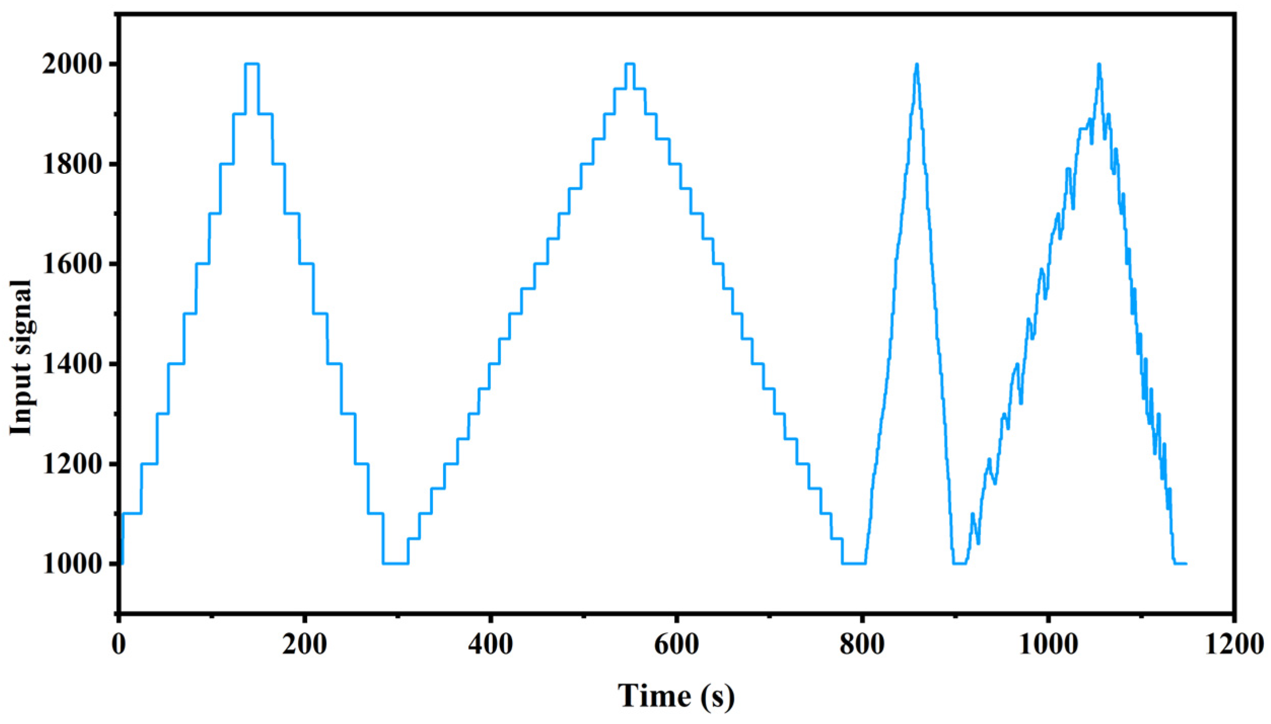
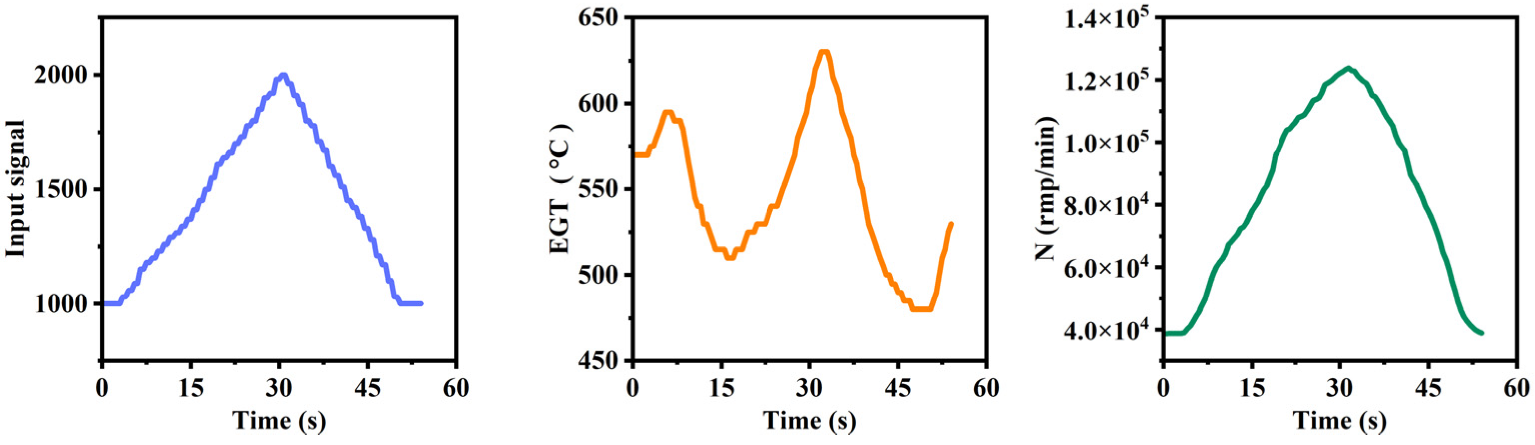
Experiments on the engine were conducted under various input conditions to prevent the training dataset from being overly homogeneous, increase dataset diversity, mitigate overfitting risks, and thus enhance the model’s generalization capability. In the experiments, the engine was subjected to step input signals of 10% and 5%, along with random signal inputs to prevent overfitting phenomena. Figure 5 illustrates the engine input signals during the experiments. Upon receiving the input signals, the micro-turbojet engine acquires operational parameters, such as the engine speed (N) (rpm/min) and exhaust gas temperature before the turbine (EGT) (°C), as depicted in Figure 6.
During the model training process, if the numerical ranges of different features differ significantly, the model tends to assign greater weights to features with larger numerical ranges and smaller weights to features with smaller numerical ranges, leading the model to be biased toward features with larger numerical ranges. Therefore, data normalization can help the model to consider each feature more evenly. In this paper, the data collected from experiments will be normalized. After normalization, the original data will be transformed into dimensionless values, avoiding the influence of significant dimensional differences, which is conducive to predicting the thrust of the engine and comprehensively evaluating the training results. Due to the significant differences in the unit magnitudes among various parameters of the engine, it is necessary to normalize the experimental data.
Normalize the input data as per Equation (10) as follows.
In the equation, x* represents the value after normalization, ximax and ximin denote the maximum and minimum values before normalization, respectively, and xi represents the data to be normalized. In this study, the entire engine dataset is divided into training and test sets in a ratio of 7:3.
In this study, data from engines operating above idle speed are chosen as inputs. This includes fuel flow rate, exhaust gas temperature, and engine speed, with thrust serving as the output.
In the equation, t denotes the current time, t − k denotes the k-th past moment, g represents the network mapping, and f(t + 1) represents the prediction of thrust at the next time step. The input data consist of the speed sequence N(t), N(t − 2), … N(t − k), the exhaust temperature sequence temp(t), temp(t − 1), … temp(t − k), and the fuel flow rate sequence W(t), W(t − 1), … W(t − k).
4. Experimental Results and Discussion
4.1. Experimental Environment Introduction
All experiments were conducted on the MATLAB 2022 platform using a PC with an Intel (R) Core (TM) i5 CPU @ 3.70 GHz, 16 GB RAM, and an NVIDIA GeForce RTX 3060Ti graphics card.
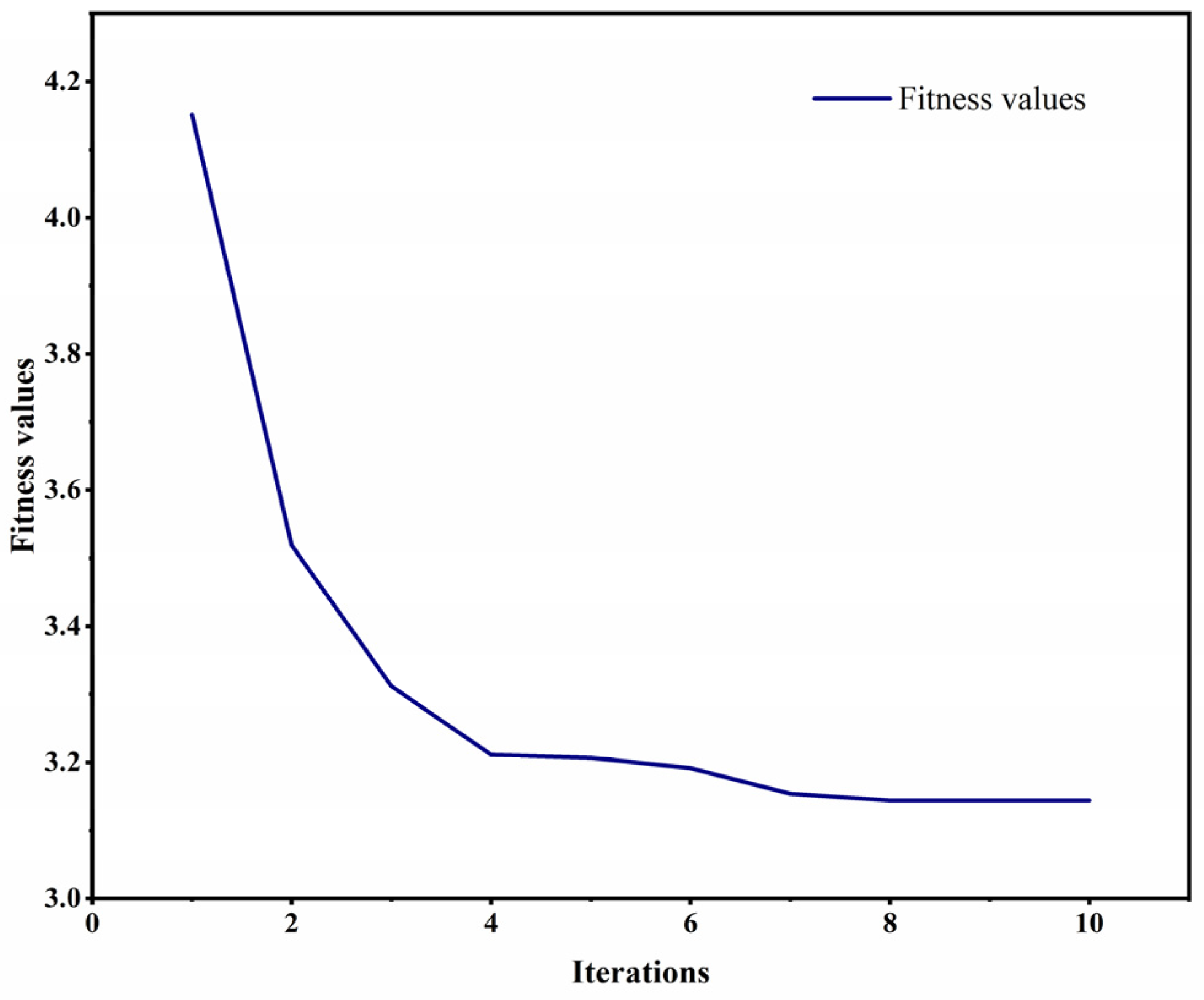
Based on the above foundation, the hyperparameters are searched as dung beetle individuals within the specified range, selecting the combination of hyperparameters with the minimum fitness function. The algorithm parameters are set as follows: the population size of DBO is 10 and the maximum number of iterations is 10. The hyperparameter search range is as follows: the range of epochs is from 40 to 100; the range of learning rate is from 0.0001 to 0.001; the range of hidden layer nodes is from 10 to 40. The hyperparameters of the proposed model are shown in Table 1.
4.2. Performance Indicators
In order to evaluate the predicted results after training, several metrics are adopted as standards for assessing the predictive performance of the model. These metrics include the mean absolute error (MAE), root-mean-square error (RMSE), and coefficient of determination (R2). The specific definitions of these metrics are as follows:
In the equations, T, q, and represent the true value, predicted value, and mean value, respectively. RMSE represents the square root error between the model’s predicted thrust and the actual thrust, and is often used as a measure of prediction accuracy. MAE is used to evaluate the deviation between the predicted and actual thrust values. R2 is used to assess the correlation between actual and predicted values, with a value closer to 1 indicating a better fit of the model to the data. Therefore, this paper integrates the aforementioned statistical indicators to evaluate the predictive performance.
4.3. Forecast Results and Discussion
In this study, DBO-CNN-BiLSTM is compared with various methods, such as CNN-BiLSTM, LSTM, GRU [57], and CNN. Also, all the methods were trained on the collected dataset five times and the average of performance metrics were calculated based on the results on the dataset. Table 2 demonstrates the experimental data results. Figure 7 shows the variation in the fitness value curve of DBO-CNN-BiLSTM.
Table 2 presents the experimental data results. The table presents the results of utilizing DBO-CNN-BiLSTM, GRU, LSTM, CNN, and CNN-BiLSTM to calculate the RMSE, MAE, and R2 of the micro-turbojet engine dataset. A higher R2 value and lower RMSE and MAE values indicate better overall performance. The results demonstrate that the proposed DBO-CNN-BiLSTM in this paper achieved an RMSE value of 0.0502, which was 19.68% lower than that of CNN-BiLSTM (0.0625), 14.48% lower than that of LSTM (0.0587), 22.41% lower than that of GRU (0.0647), and 20.98% lower than that of CNN (0.0636). For the MAE value, the performance improvement was significant, with DBO-CNN-BiLSTM achieving a value of 0.0391, which was the smallest among the compared models, representing reductions of 19.54%, 8.86%, 20.45%, and 23.14% compared with those of GRU, LSTM, CNN, and CNN-BiLSTM, respectively. Additionally, DBO-CNN-BiLSTM achieved an R2 value of 0.9924, which was the highest compared with the others, indicating a higher level of prediction stability.
In order to better evaluate the thrust estimation of DBO-CNN-BiLSTM, engine experimental data at different time points of engine operation were introduced in this study to evaluate the performance of the model. In Experiment A, a large step signal was input to the engine to obtain experimental data for approximately 184 s. Figure 8 shows the thrust prediction results of DBO-CNN-BiLSTM and other models. The figure plots the actual test thrust values and the predicted values of each model. The black color represents the actual values tested on the test stand, while the red color represents the predictions made by DBO-CNN-BiLSTM.
Figure 8 illustrates that, after the input of a larger step signal, the thrust value rose rapidly and then stabilized at a certain level. Fluctuations occurred in the predictions of all models during the rising phase. During the subsequent steady-state phase, the predicted values of DBO-CNN-BiLSTM were closer to the experimental test values. The fluctuations may have been due to unstable data changes in a rapidly changing state. To better evaluate the predictive performance of the model, we introduced MAE and RMSE, mean error, and maximum error as evaluation metrics. The percentage error was calculated as the percentage absolute value of a fraction of the maximum thrust achievable by the turbojet engine. As shown in Table 3, in this experiment, the MAE value of DBO-CNN-BiLSTM was 0.0406, 7.11% lower than that of CNN-BiLSTM (0.0437), approximately 10.57% lower than that of LSTM (0.0454), and 25.37% lower than that of CNN. For RMSE, the value of DBO-CNN-BiLSTM in this experiment was 0.0651, the lowest among other methods, with the largest decrease compared with GRU (0.0840) being 22.5%. The mean error obtained by DBO-CNN-BiLSTM was 2.01%, and the maximum error was 8.71% in the face of larger state transitions, which rose little in comparison with the other models. The error rose at larger state transitions, possibly caused by faster state transitions that resulted in unstable temperature changes inside the engine.
In Experiment B, we input a smaller step signal to the engine for a duration of about 200 s. The results of each model for the Experiment B data are shown in Figure 9. The corresponding evaluation metrics are shown in Table 4. With the smaller step input, both MAE and RMSE showed a decrease compared with Experiment A. Specifically, DBO-CNN-BiLSTM achieved an MAE of 0.0410, which was 13.87% lower than that of GRU (0.0476), and decreases of 9.49% and 9.89% compared with those of CNN-BiLSM (0.453) and LSTM (0.455), respectively. In terms of RMSE, there was a maximum reduction of 17.55% compared with GRU (0.587). The mean error of DBO-CNN-BiLSTM was 2.03%, which was 9.78% lower than that of GRU (2.35%). The maximum error of the model in this paper was also kept lower than other models under smaller state changes.
For Experiment C, involving continuous acceleration and deceleration of the engine for approximately 107 s, the predictive results of each model are shown in Figure 10. Based on the evaluation metrics in Table 5, it is observed that both MAE and RMSE increased compared with the previous two experiments. The MAE value of the proposed method was 0.0478 compared with the other methods. Although the RMSE obtained in this experiment also increased compared with the experiments with continuous step inputs, the proposed method showed a decrease of 9.13% compared with CNN-BiLSTM and 10.47% compared with LSTM. The mean error of DBO-CNN-BiLSTM was less variable compared with other models.
The data indicate that, when faced with irregular controls, DBO-CNN-BiLSTM obtained lower MAE and RMSE values compared with other algorithms. This indicates that the model could capture local features within the input sequences, thereby enhancing its performance in the face of complex variations. Three experiments compared the predictive performance of the model under different conditions and compared it with other models. Among several evaluation metrics, DBO-CNN-BiLSTM achieved better results than the other models. The models fluctuated when faced with acceleration and deceleration state switching with fast speeds, which may have been due to the unstable changes during the state transition while the temperature distribution inside the engine was uneven or the transfer of the temperature change rate was relatively slow, as well as the vibration caused by the changes in the engine at high speeds.
5. Conclusions
The paper proposes a CNN-BiLSTM network optimized by DBO for thrust estimation of micro-turbojet engines. CNN can better extract latent features from the data of the engine, while BiLSTM analyzes the dependency between the data, thereby improving the model’s ability to capture the time-series characteristics of the micro-turbojet engine data. DBO optimizes the training hyperparameters of the model, further enhancing the model’s performance prediction capability and accuracy for the micro-turbojet engine. DBO-CNN-BiLSTM was compared with other models on the test dataset, and metrics such as RMSE and R2 were used to evaluate the model. In addition, the model was tested under different step inputs and analyzed by four metrics: MAE, RSME, mean error, and maximum error, and the data showed that the optimum was obtained in three experiments. The mean error was lower than that of the other models. Although the MAE and RSME of all models increased in response to continuous input variations, DBO-CNN-BiLSTM outperformed the other models under irregular input testing, achieving lower MAE and RMSE values. In future work, we will consider additional factors, including environmental conditions such as ambient pressure, and adjust the model to incorporate these factors in order to further improve its predictive accuracy under different environmental conditions.
Author Contributions
Conceptualization, H.H.; Validation, B.L.; Investigation, H.L.; Data curation, G.C.; Writing—original draft, B.L.; Writing—review & editing, J.L.; Supervision, H.H. All authors have read and agreed to the published version of the manuscript.
Funding
This work is supported by the National Natural Science Foundation of China (52366007) and the Guangxi Science and Technology Major Project (AA22068103, AA22068104).
Data Availability Statement
The raw data supporting the conclusions of this article will be made available by the authors on request.
Conflicts of Interest
We declare that we do not have any commercial or associative interests that represents a conflict of interest in connection with the work submitted.
References
- Mohsan, S.A.H.; Khan, M.A.; Noor, F.; Ullah, I.; Alsharif, M.H. Towards the Unmanned Aerial Vehicles (UAVs): A Comprehensive Review. Drones 2022, 6, 147. [Google Scholar] [CrossRef]
- Kikutis, R.; Stankūnas, J.; Rudinskas, D. Evaluation of UAV autonomous flight accuracy when classical navigation algorithm is used. Transport 2018, 33, 589–597. [Google Scholar] [CrossRef]
- Large, J.; Pesyridis, A. Investigation of Micro Gas Turbine Systems for High Speed Long Loiter Tactical Unmanned Air Systems. Aerospace 2019, 6, 55. [Google Scholar] [CrossRef]
- Oppong, F.; Van Der Spuy, S.J.; Diaby, A.L. An overview on the performance investigation and improvement of micro gas turbine engine. R D J. S. Afr. Inst. Mech. Eng. 2015, 31, 35–41. [Google Scholar]
- Turan, O. Exergetic effects of some design parameters on the small turbojet engine for unmanned air vehicle applications. Energy 2012, 46, 51–61. [Google Scholar] [CrossRef]
- Nava, G.; Fiorio, L.; Traversaro, S.; Pucci, D. Position and Attitude Control of an Underactuated Flying Humanoid Robot. In Proceedings of the 2018 IEEE-RAS 18th International Conference on Humanoid Robots (Humanoids), Beijing, China, 6–9 November 2018; IEEE: Piscataway, NJ, USA, 2018; pp. 1–9. [Google Scholar]
- Mohamed, H.A.O.; Nava, G.; L’Erario, G.; Traversaro, S.; Bergonti, F.; Fiorio, L.; Vanteddu, P.R.; Braghin, F.; Pucci, D. Momentum-Based Extended Kalman Filter for Thrust Estimation on Flying Multibody Robots. IEEE Robot. Autom. Lett. 2022, 7, 526–533. [Google Scholar] [CrossRef]
- Fu, M.; Guo, Q.; Cheng, Z. Structural Design and Finite Element Analysis of a Vortex Jet Power Vehicle. In Proceedings of the 2019 International Conference on Robotics, Intelligent Control and Artificial Intelligence (RICAI 2019), Shanghai, China, 20–22 September 2019; pp. 706–711. [Google Scholar]
- Jie, M.S.; Mo, E.J.; Hong, G.Y.; Lee, K.W. Fuzzy logic controller for turbojet engine of unmanned aircraft. In Knowledge-Based Intelligent Information and Engineering Systems; Part 1, Proceedings; Springer: Berlin/Heidelberg, Germany, 2006; Volume 4251, pp. 29–36. [Google Scholar]
- Amirante, R.; Catalano, L.A.; Tamburrano, P. Thrust Control of Small Turbojet Engines Using Fuzzy Logic: Design and Experimental Validation. J. Eng. Gas Turbines Power 2012, 134, 121601. [Google Scholar] [CrossRef]
- Henriksson, M.; Grönstedt, T.; Breitholtz, C. Model-based on-board turbofan thrust estimation. Control Eng. Pract. 2011, 19, 602–610. [Google Scholar] [CrossRef]
- Litt, J.S. An optimal orthogonal decomposition method for Kalman filter-based turbofan engine thrust estimation. J. Eng. Gas Turbines Power 2008, 130, 011601. [Google Scholar] [CrossRef]
- Zhu, Y.; Huang, J.; Pan, M.; Zhou, W. Direct thrust control for multivariable turbofan engine based on affine linear parameter-varying approach. Chin. J. Aeronaut. 2022, 35, 125–136. [Google Scholar] [CrossRef]
- Simon, D.L.; Borguet, S.; Leonard, O.; Zhang, X.F. Aircraft Engine Gas Path Diagnostic Methods: Public Benchmarking Results. J. Eng. Gas Turbines Power 2014, 136, 041201. [Google Scholar] [CrossRef]
- De Giorgi, M.G.; Quarta, M. Hybrid Multigene Genetic Programming—Artificial neural networks approach for dynamic performance prediction of an aeroengine. Aerosp. Sci. Technol. 2020, 103, 105902. [Google Scholar] [CrossRef]
- KrishnaKumar, K.; Yachisako, Y.; Huang, Y. Jet engine performance estimation using intelligent system technologies. In Proceedings of the 39th Aerospace Sciences Meeting and Exhibit, Reno, NV, USA, 8–11 January 2001; p. 1122. [Google Scholar]
- Liu, Y.N.; Zhang, S.X.; Zhang, C. Aero engine thrust estimator design based on kernel method. J. Propuls. Technol. 2013, 34, 829–835. [Google Scholar]
- Cortes, C.; Vapnik, V. Support-vector networks. Mach. Learn. 1995, 20, 273–297. [Google Scholar] [CrossRef]
- Song, H.Q.; Li, B.W.; Zhang, Y.; Jiang, K.Y. Aero-engine thrust estimator design based on clustering and particle swarm optimization extreme learning machine. Tuijin Jishu/J. Propuls. Technol. 2017, 38, 1379–1385. [Google Scholar]
- Kennedy, J.; Eberhart, R. Particle swarm optimization. In Proceedings of the ICNN’95—International Conference on Neural Networks, Perth, WA, Australia, 27 November–1 December 1995; IEEE: Piscataway, NJ, USA, 1995; pp. 1942–1948. [Google Scholar]
- Huang, G.; Zhu, Q.; Siew, C. Extreme learning machine: Theory and applications. Neurocomputing 2006, 70, 489–501. [Google Scholar] [CrossRef]
- Li, Z.; Zhao, Y.; Cai, Z.; Xi, P.; Pan, Y.; Huang, G.; Zhang, T. A proposed self-organizing radial basis function network for aero-engine thrust estimation. Aerosp. Sci. Technol. 2019, 87, 167–177. [Google Scholar] [CrossRef]
- Zhao, Y.; Chen, Y.; Li, Z. A proposed algorithm based on long short-term memory network and gradient boosting for aeroengine thrust estimation on transition state. Proc. Inst. Mech. Eng. Part G J. Aerosp. Eng. 2021, 235, 2182–2192. [Google Scholar] [CrossRef]
- Siami-Namini, S.; Tavakoli, N.; Namin, A.S. The Performance of LSTM and BiLSTM in Forecasting Time Series. In Proceedings of the 2019 IEEE International Conference on Big Data (Big Data), Los Angeles, CA, USA, 9–12 December 2019; IEEE: Piscataway, NJ, USA; pp. 3285–3292. [Google Scholar]
- Momin, A.J.A.; Nava, G.; L’Erario, G.; Mohamed, H.A.O.; Bergonti, F.; Vanteddu, P.R.; Braghin, F.; Pucci, D. Nonlinear Model Identification and Observer Design for Thrust Estimation of Small-scale Turbojet Engines. In Proceedings of the 2022 IEEE International Conference On Robotics and Automation (ICRA 2022), Philadelphia, PA, USA, 23–27 May 2022; pp. 5879–5885. [Google Scholar]
- Tang, W.; Wang, L.; Gu, J.; Gu, Y. Single Neural Adaptive PID Control for Small UAV Micro-Turbojet Engine. Sensors 2020, 20, 345. [Google Scholar] [CrossRef] [PubMed]
- Shehata, A.M.; Khalil, M.K.; Ashry, M.M. Adaptive Fuzzy PID Controller applied to micro turbojet engine. J. Phys. Conf. Ser. 2021, 2128, 012030. [Google Scholar] [CrossRef]
- Altarazi, Y.S.M.; Abu Talib, A.R.; Gires, E.; Yu, J.; Lucas, J.; Yusaf, T. Performance and exhaust emissions rate of small-scale turbojet engine running on dual biodiesel blends using Gasturb. Energy 2021, 232, 120971. [Google Scholar] [CrossRef]
- Balli, O.; Kale, U.; Rohács, D.; Karakoc, T.H. Exergoenvironmental, environmental impact and damage cost analyses of a micro turbojet engine (m-TJE). Energy Rep. 2022, 8, 9828–9845. [Google Scholar] [CrossRef]
- Xu, Y.; Gao, L.; Cao, R.; Yan, C.; Piao, Y. Power Balance Strategies in Steady-State Simulation of the Micro Gas Turbine Engine by Component-Coupled 3D CFD Method. Aerospace 2023, 10, 782. [Google Scholar] [CrossRef]
- Cican, G.; Frigioescu, T.; Crunteanu, D.; Cristea, L. Micro Turbojet Engine Nozzle Ejector Impact on the Acoustic Emission, Thrust Force and Fuel Consumption Analysis. Aerospace 2023, 10, 162. [Google Scholar] [CrossRef]
- Hochreiter, S.; Schmidhuber, J. Long Short-Term Memory. Neural Comput. 1997, 9, 1735–1780. [Google Scholar] [CrossRef] [PubMed]
- Sherstinsky, A. Fundamentals of Recurrent Neural Network (RNN) and Long Short-Term Memory (LSTM) network. Phys. D Nonlinear Phenom. 2020, 404, 132306. [Google Scholar] [CrossRef]
- Lu, W.; Li, J.; Wang, J.; Qin, L. A CNN-BiLSTM-AM method for stock price prediction. Neural Comput. Appl. 2021, 33, 4741–4753. [Google Scholar] [CrossRef]
- Antonius, F.; Sekhar, J.C.; Sreenivasa Rao, V.; Pradhan, R.; Narendran, S.; Fernando Cosio Borda, R.; Silvera-Arcos, S. Unleashing the power of Bat optimized CNN-BiLSTM model for advanced network anomaly detection: Enhancing security and performance in IoT environments. Alex. Eng. J. 2023, 84, 333–342. [Google Scholar] [CrossRef]
- Ramshankar, N.; Joe Prathap, P.M. Automated sentimental analysis using heuristic-based CNN-BiLSTM for E-commerce dataset. Data Knowl. Eng. 2023, 146, 102194. [Google Scholar] [CrossRef]
- Muhammad, K.; Mustaqeem; Ullah, A.; Imran, A.S.; Sajjad, M.; Kiran, M.S.; Sannino, G.; de Albuquerque, V.H.C. Human action recognition using attention based LSTM network with dilated CNN features. Future Gener. Comput. Syst. 2021, 125, 820–830. [Google Scholar] [CrossRef]
- Aslan, M.F.; Unlersen, M.F.; Sabanci, K.; Durdu, A. CNN-based transfer learning—BiLSTM network: A novel approach for COVID-19 infection detection. Appl. Soft Comput. 2021, 98, 106912. [Google Scholar] [CrossRef] [PubMed]
- Mellit, A.; Pavan, A.M.; Lughi, V. Deep learning neural networks for short-term photovoltaic power forecasting. Renew. Energ. 2021, 172, 276–288. [Google Scholar] [CrossRef]
- Guo, X.; Bi, Z.; Wang, J.; Qin, S.; Liu, S.; Qi, L. Reinforcement learning for disassembly system optimization problems: A survey. Int. J. Netw. Dyn. Intell. 2023, 2, 1–14. [Google Scholar] [CrossRef]
- Kim, T.; Cho, S. Optimizing CNN-LSTM neural networks with PSO for anomalous query access control. Neurocomputing 2021, 456, 666–677. [Google Scholar] [CrossRef]
- Sekhar, C.; Dahiya, R. Robust framework based on hybrid deep learning approach for short term load forecasting of building electricity demand. Energy 2023, 268, 126660. [Google Scholar] [CrossRef]
- Xue, J.; Shen, B. Dung beetle optimizer: A new meta-heuristic algorithm for global optimization. J. Supercomput. 2022, 79, 7305–7336. [Google Scholar] [CrossRef]
- Zhang, R.; Zhu, Y. Predicting the Mechanical Properties of Heat-Treated Woods Using Optimization-Algorithm-Based BPNN. Forests 2023, 14, 935. [Google Scholar] [CrossRef]
- Yoo, Y.; Baek, J. A Novel Image Feature for the Remaining Useful Lifetime Prediction of Bearings Based on Continuous Wavelet Transform and Convolutional Neural Network. Appl. Sci. 2018, 8, 1102. [Google Scholar] [CrossRef]
- Ilesanmi, A.E.; Ilesanmi, T.O. Methods for image denoising using convolutional neural network: A review. Complex Intell. Syst. 2021, 7, 2179–2198. [Google Scholar] [CrossRef]
- Khan, A.; Sohail, A.; Zahoora, U.; Qureshi, A.S. A survey of the recent architectures of deep convolutional neural networks. Artif. Intell. Rev. 2020, 53, 5455–5516. [Google Scholar] [CrossRef]
- Swapna, G.; Kp, S.; Vinayakumar, R. Automated detection of diabetes using CNN and CNN-LSTM network and heart rate signals. Procedia Comput. Sci. 2018, 132, 1253–1262. [Google Scholar]
- Kamalov, F. Forecasting significant stock price changes using neural networks. Neural Comput. Appl. 2020, 32, 17655–17667. [Google Scholar] [CrossRef]
- Zhang, G.; Bai, X.; Wang, Y. Short-time multi-energy load forecasting method based on CNN-Seq2Seq model with attention mechanism. Mach. Learn. Appl. 2021, 5, 100064. [Google Scholar] [CrossRef]
- Kim, T.; Cho, S. Predicting residential energy consumption using CNN-LSTM neural networks. Energy 2019, 182, 72–81. [Google Scholar] [CrossRef]
- Cheng, H.; Ding, X.; Zhou, W.; Ding, R. A hybrid electricity price forecasting model with Bayesian optimization for German energy exchange. Int. J. Electr. Power 2019, 110, 653–666. [Google Scholar] [CrossRef]
- Wu, K.; Wu, J.; Feng, L.; Yang, B.; Liang, R.; Yang, S.; Zhao, R. An attention-based CNN-LSTM-BiLSTM model for short-term electric load forecasting in integrated energy system. Int. Trans. Electr. Energy Syst. 2021, 31, e12637. [Google Scholar] [CrossRef]
- Gao, W.; Liu, S. Improved artificial bee colony algorithm for global optimization. Inf. Process Lett. 2011, 111, 871–882. [Google Scholar] [CrossRef]
- Sun, R. Optimization for Deep Learning: An Overview. J. Oper. Res. Soc. China 2020, 8, 249–294. [Google Scholar] [CrossRef]
- Abou Houran, M.; Salman Bukhari, S.M.; Zafar, M.H.; Mansoor, M.; Chen, W. COA-CNN-LSTM: Coati optimization algorithm-based hybrid deep learning model for PV/wind power forecasting in smart grid applications. Appl. Energ. 2023, 349, 121638. [Google Scholar] [CrossRef]
- Cho, K.; Merrienboer, B.V.; Gulcehre, C.; Bahdanau, D.; Bougares, F.; Schwenk, H.; Bengio, Y. Learning Phrase Representations Using RNN Encoder-Decoder for Statistical Machine Translation; Cornell University Library: Ithaca, NY, USA, 2014; Available online: https://arxiv.org/abs/1406.1078 (accessed on 18 April 2024).
Figure 1.
CNN model structure diagram.

Figure 2.
Schematic diagram of BiLSTM structure.

Figure 3.
DBO-CNN-BiLSTM Flowchart.

Figure 4.
Schematic structure of the micro-turbojet engine test platform.

Figure 5.
Engine input signal.

Figure 6.
Partial data during test.

Figure 7.
Fitness value curve.

Figure 8.
Comparison of results from experiment A.

Figure 9.
Comparison of results from experiment B.

Figure 10.
Comparison of results from experiment C.


Table 1.
The hyperparameters.
| Methods | Value |
|---|---|
| DBO-CNN-BiLSTM | optimal hyper-parameter combination is obtained by DBO. activation function (RELU). pooling layer activation function (RELU) |
| CNN-BiLSTM | batch size (128) learning rate (0.001) hidden nodes (100) activation function (RELU) pooling layer activation function (RELU) |
| CNN | batch size (128) learning rate (0.001) activation function (RELU) pooling layer activation function (RELU) |
| LSTM | batch size (128) hidden nodes (100) learning rate (0.001) activation function (RELU) |
| GRU | batch size (128) hidden nodes (100) learning rate (0.001) activation function (RELU) |
Table 2.
Comparison results with other models.
| Evaluation Metrics | DBO-CNN-BiLSTM | GRU | LSTM | CNN | CNN-BiLSTM |
|---|---|---|---|---|---|
| RSME | 0.0502 | 0.0647 | 0.0587 | 0.0636 | 0.0625 |
| MAE | 0.0391 | 0.0486 | 0.0429 | 0.0492 | 0.0508 |
| R2 | 0.9924 | 0.9834 | 0.9901 | 0.9885 | 0.9884 |
Table 3.
Results from experiment A.
| Evaluation Metrics | DBO-CNN-BiLSTM | GRU | LSTM | CNN | CNN-BiLSTM |
|---|---|---|---|---|---|
| MAE | 0.0406 | 0.0509 | 0.0454 | 0.0544 | 0.0437 |
| RSME | 0.0651 | 0.0840 | 0.0717 | 0.0762 | 0.0662 |
| Mean Error | 2.01% | 2.52% | 2.21% | 2.69% | 2.16% |
| Maximum Error | 8.71% | 11.79% | 10.58% | 11.50% | 9.76% |
Table 4.
Results from experiment B.
| Evaluation Metrics | DBO-CNN-BiLSTM | GRU | LSTM | CNN | CNN-BiLSTM |
|---|---|---|---|---|---|
| MAE | 0.0410 | 0.0476 | 0.0455 | 0.0469 | 0.0453 |
| RSME | 0.0484 | 0.0587 | 0.0549 | 0.0548 | 0.0554 |
| Mean Error | 2.03% | 2.35% | 2.25% | 2.32% | 2.24% |
| Max Error | 8.05% | 9.49% | 10.14% | 10.67% | 8.91% |
Table 5.
Results from experiment C.
| Evaluation Metrics | DBO-CNN-BiLSTM | GRU | LSTM | CNN | CNN-BiLSTM |
|---|---|---|---|---|---|
| MAE | 0.0478 | 0.0632 | 0.0569 | 0.0627 | 0.0521 |
| RSME | 0.0608 | 0.0759 | 0.0679 | 0.1048 | 0.0669 |
| Mean Error | 2.10% | 3.13% | 2.81% | 3.10% | 2.57% |
| Max Error | 8.24% | 9.67% | 9.31% | 10.07% | 9.08% |
Disclaimer/Publisher’s Note: The statements, opinions and data contained in all publications are solely those of the individual author(s) and contributor(s) and not of MDPI and/or the editor(s). MDPI and/or the editor(s) disclaim responsibility for any injury to people or property resulting from any ideas, methods, instructions or products referred to in the content. |
© 2024 by the authors. Licensee MDPI, Basel, Switzerland. This article is an open access article distributed under the terms and conditions of the Creative Commons Attribution (CC BY) license (https://creativecommons.org/licenses/by/4.0/).
Share and Cite
MDPI and ACS Style
Lei, B.; Huang, H.; Chen, G.; Liang, J.; Long, H. DBO-CNN-BiLSTM: Dung Beetle Optimization Algorithm-Based Thrust Estimation for Micro-Aero Engine. Aerospace 2024, 11, 344. https://doi.org/10.3390/aerospace11050344
AMA Style
Lei B, Huang H, Chen G, Liang J, Long H. DBO-CNN-BiLSTM: Dung Beetle Optimization Algorithm-Based Thrust Estimation for Micro-Aero Engine. Aerospace. 2024; 11(5):344. https://doi.org/10.3390/aerospace11050344
Chicago/Turabian StyleLei, Baijun, Haozhong Huang, Guixin Chen, Jianguo Liang, and Huigui Long. 2024. "DBO-CNN-BiLSTM: Dung Beetle Optimization Algorithm-Based Thrust Estimation for Micro-Aero Engine" Aerospace 11, no. 5: 344. https://doi.org/10.3390/aerospace11050344
Note that from the first issue of 2016, this journal uses article numbers instead of page numbers. See further details here.