Article

Transmit Energy Efficiency of Two Cognitive Radar Platforms for Target Identification

Department of Electrical and Computer Engineering, Naval Postgraduate School, Monterey, CA 93943, USA
*
Author to whom correspondence should be addressed.
Aerospace 2015, 2(3), 376-391; https://doi.org/10.3390/aerospace2030376
Submission received: 31 March 2015 / Revised: 29 May 2015 / Accepted: 29 May 2015 / Published: 26 June 2015
(This article belongs to the Special Issue Driving Forward Aerospace Innovation)

Abstract

:
Cognitive radar (CRr) is a recent radar paradigm that can potentially help drive aerospace innovation forward. Two specific platforms of cognitive radar used for target identification are discussed. One uses sequential hypothesis testing (SHT) in the receiver processing and is referred to as SHT-CRr and the other one uses maximum a posteriori (MAP) and is referred to as MAP-CRr. Our main goal in this article is to make a practical comparison between SHT-CRr and MAP-CRr platforms in terms of transmission energy efficiency. Since the performance metric for the SHT-CRr is the average number of illuminations (ANI) and the performance metric for MAP-CRr is the percentage of correct decisions ( P c d ), a direct comparison between the platforms is difficult to perform. In this work, we introduce a useful procedure that involves a metric called total transmit energy (TTE) given a fixed P c d as a metric to measure the transmit energy efficiency of both platforms. Lower TTE means that the platform is more efficient in achieving a desired P c d . To facilitate a robust comparison, a transmit-adaptive waveform that consistently outperforms the pulsed waveform in terms of both P c d and ANI is needed. We show that a certain adaptive waveform called the probability weighted energy signal-to-noise ratio-based (PWE-SNR) waveform outperforms the pulsed wideband waveform (i.e., flat frequency response) in terms of ANI and P c d for all ranges of transmit waveform energy. We also note that the P c d performance of SHT-CRr can be drastically different from the probability threshold (i.e., the probability value that is used to stop radar illumination for the purposes of classification), which is critically important for CRr system designers to realize. Indeed, this fact turns out to be key in accomplishing our goal to compare SHT-CRr and MAP-CRr in terms of transmit energy efficiency.

Graphical Abstract

1. Introduction

The use of radar in aerospace engineering is very widespread and has a very long history. It is a futile task to cite all relevant works in various applications, but we will mention a few good ones for the novice and interested reader. For example, radar is used in navigation [1,2]. Of course, one major contribution of radar is in air traffic control [3,4]. Moreover some planes (commercial or military) have radars used for safety and/or aviation, i.e., radars that warn pilots of other planes, weather and/or targets [5]. Other radars installed in airborne applications are used for imaging, such as synthetic aperture radar (SAR) [6,7]. Others are used for remote sensing [8,9]. The list goes on and on. Our interest here is a radar application that is used for target identification. More specifically, we are interested in a closed-loop radar that is able to dynamically change its waveform for the purposes of target identification. Such a radar uses information extracted from previously received signals to adaptively modify its waveform to efficiently identify the present target in an identification scenario. This radar is an example of a closed-loop radar system, also known as cognitive radar (CRr) [10,11]. A knowledge-aided approach for CRr is presented in [12], and a knowledge-aided waveform and receiver filter design is presented in [13].
In [14], two types of cognitive radar (CRr) platforms were introduced for target identification with the use of adaptive transmit waveforms. These two platforms were extended for stochastic targets in [15] for the purposes of target classification, i.e., the radar is used to classify which target class a particular target belongs to. These platforms were extended in the case of signal-dependent interference [16,17]. The two CRrs are different (from the receiver signal processing point of view) since each uses a different metric to measure the CRr’s performance. The first type of CRr assumes a fixed probability threshold and finds the average number of illuminations (ANI) or transmissions to meet that threshold as a function of transmit waveform energy level (which can easily be translated to the power constraint). Sequential hypothesis testing (SHT) is used in the receiver, and as such, we label this radar as SHT-CRr. The second CRr does not use a probability threshold. Instead, it assumes a fixed number of transmissions. The metric used is the probability of correct identification or the percentage of correct decision ( P c d ). Here, maximum a posteriori (MAP) is used to decide which target is present in a target identification scenario. As such, we call this platform MAP-CRr.
Our goal in this article is to make a practical comparison between SHT-CRr and MAP-CRr platforms. Because the performance metrics are different, it is difficult to make a direct comparison between the two. A recent and important push in electronic and aerospace systems is that a system or subsystem be energy efficient, also known as a green system or technology. Therefore, one of the more important contributions of this paper is to introduce a useful procedure and energy metric, such that that energy efficiency for both waveforms can be quantified, and thus, a comparison can be made as to which platform is more transmit energy efficient. However in most target recognition applications, P c d is an important requirement in practice. Thus, we will compare the two CRrs in terms of energy efficiency given a fixed P c d . In [14,15,16], various adaptive waveforms performed better in terms of ANI and P c d compared to the wideband waveform, but interestingly, not in all ranges of transmit energy. To facilitate a robust comparison, a waveform that consistently outperforms the classical pulsed wideband waveform as a function of transmit energy per pulse is needed. In [18], a certain probability-weighted energy (PWE) signal-to-noise ratio-based waveform was proposed. This PWE-SNR waveform showed good preliminary results in terms of P c d , but no results were shown for ANI, which we need for our comparison study. Therefore, to compare SHT-CRr and MAP-CRr, another contribution of this paper is to produce performance results in terms of both P c d and ANI for the PWE-SNR waveform and to show that it indeed performs better than the wideband waveform for all transmit energy levels. We also report in this work that the resulting P c d of SHT-CRr can be drastically different from the probability threshold used (as a function of transmit energy). This result is important to report, so that designers in the radar community may know at what levels of energy are or what power is needed when the resulting P c d is much lower than the probability threshold used. If we indeed require that P c d match (or be even greater than) the probability threshold used, then we need the transmit energy levels (i.e., SNR range) in which this is true, such that we can meet this P c d requirement.
This paper is organized as follows. Section 2 introduces the need, procedure and metric, such that two types of cognitive radar for target recognition may be compared. Section 3 provides a review of the two radars, which are named SHT-CRr and MAP-CRr. Section 3.1 introduces the notion of the matched illumination waveform, called the eigen-waveform. Section 3.2 frames the target recognition problem in terms of multiple hypothesis testing (MHT). Section 3.3 discusses how a transmit adaptive waveform can be formed. Section 3.4 discusses how initial priors are updated via past and current measurements. Section 3.5 discusses how SHT-CRr and MAP-CRr differ in terms of signal processing and performance metrics. Section 4 discusses the two metrics of interest: P c d and ANI. Section 5 shows the performance results and compares the radars in terms of the metric total transmit energy (TTE). Section 6 concludes the paper.

2. Procedure and Metric to Compare MAP-CRr and SHT-CRr

While it is clear in [14,15,16,17,18] that the two CRr platforms are better than conventional systems, it is not clear which one of the two CRr platforms is better and how to even compare them. This is because a direct comparison of their metrics is difficult since the performance metrics are inherently different. In a multiple target hypothesis testing problem, the MAP-CRr tries to identify the correct hypothesis after a fixed number of illuminations instead of using a probability threshold. The resulting performance metric is called the probability of correct identification or the percentage of correct decisions ( P c d ) . To generate performance results, we utilize Monte Carlo simulations to calculate the percentage of correct decisions, and thus, we will refer to the P c d metric for MAP-CRr. The SHT-CRr does not limit the number of illuminations. Instead, it uses a probability threshold to stop the transmissions. The random nature of the noise in the receiver makes the number of illuminations different from experiment to experiment, i.e., random. Therefore, the performance metric is the average number of illuminations (ANI). In a Monte Carlo target identification simulation, ANI refers to the mean number of transmissions it takes for a hypothesis probability to cross a given probability threshold (since there is a vast number of experiments used).
The receiver nature of the two platforms may be different, but in the end, an important requirement (if not the most important) in target identification is the eventual P c d . In other words, we need not only find the ANI for SHT-CRr, but the actual P c d corresponding to the ANI. Recall that the SHT-CRr uses a probability threshold to stop illumination and makes a decision as to which target is present. Unfortunately, the probability threshold does not necessarily yield the P c d desired, as will be shown in this work. Thus, to make a fair comparison, we propose to compare the total transmit energy (TTE) spent on yielding that P c d . Total transmit energy is needed, because each platform uses multiple transmissions. In other words, the less total transmit energy spent in producing that P c d , the more efficient that type of radar is. For the MAP-CRr, TTE is the number of transmission times the energy level used (given a certain P c d , number of transmissions and waveform type). For the SHT-CRr, the “average” total transmit energy (TTE) is the corresponding ANI times the energy level per transmission pulse (again for a certain P c d ) given a fixed probability threshold.
Unlike the number or illuminations or probability threshold, it is difficult to fix the P c d in a Monte Carlo simulation. Therefore, we propose the following “procedure” in order to find TTE and, thus, perform the energy efficiency comparison: (1) set up a Monte Carlo target identification simulation using SHT-CRr given a probability threshold to plot ANI vs. transmit energy results; (2) calculate and plot the corresponding P c d vs. transmit energy for that experiment; (3) set up a Monte Carlo simulation using MAP-CRr to produce P c d vs. the transmit energy plot using various numbers of transmissions; (4) from the SHT-CRr’s P c d vs. transmit energy plot, pick a specific transmit energy level (this may start with a low energy level); note the corresponding P c d (to be used for comparison); note the resulting ANI; then calculate the SHT-CRr’s TTE for that P c d ; (5) now, using the same energy level (used in SHT-CRr), find the number of transmissions that has the closest P c d noted above and calculate MAP-CRr’s TTE; (6) decide that whichever radar has the lower TTE is the the more efficient type; and (7) repeat the process for medium and high energy levels to see if one type is consistently more efficient than the other. To illustrate the procedure, example results will be analyzed in Section 5 (Comparing TTE).

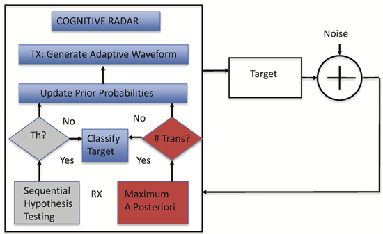
3. Brief Review of the Two Types of CRr

Both SHT-CRr and MAP-CRr are used for the target recognition problem. They share common features, as shown in Figure 1. Notice that what makes a radar system cognitive is the the closed-loop nature of the system. Notice that both types of radar update the prior probabilities of the target hypotheses. These updated probabilities (calculated from the latest measurements) are passed from the receiver to the transmitter portion of the radar. Due to the Bayesian nature of updating these probabilities, these probability updates also incorporate prior measurements (which means that prior knowledge is retained, making the system cognitive). These probability updates are used in generating the next waveform to illuminate the radar scene, thereby closing the loop. Since the updated probabilities are different, the new waveform is also different, making it truly transmit adaptive. To describe this closed-loop system in detail, we need a brief review of the signal processing models used in Figure 1.
Figure 1. Block diagram of sequential hypothesis testing (SHT)-cognitive radar (CRr) and MAP-CRr for target recognition or identification application.
Aerospace 02 00376 g001

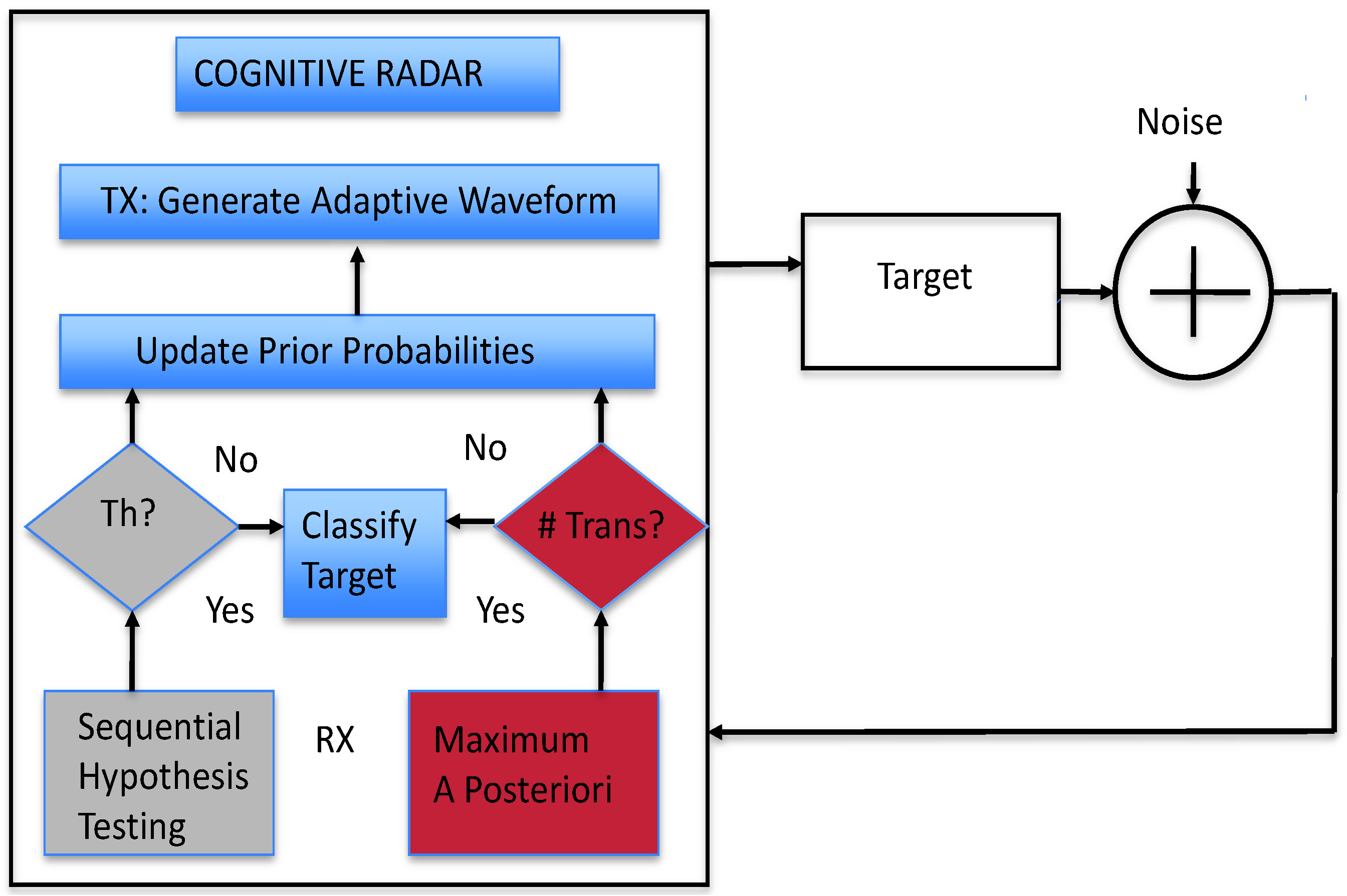
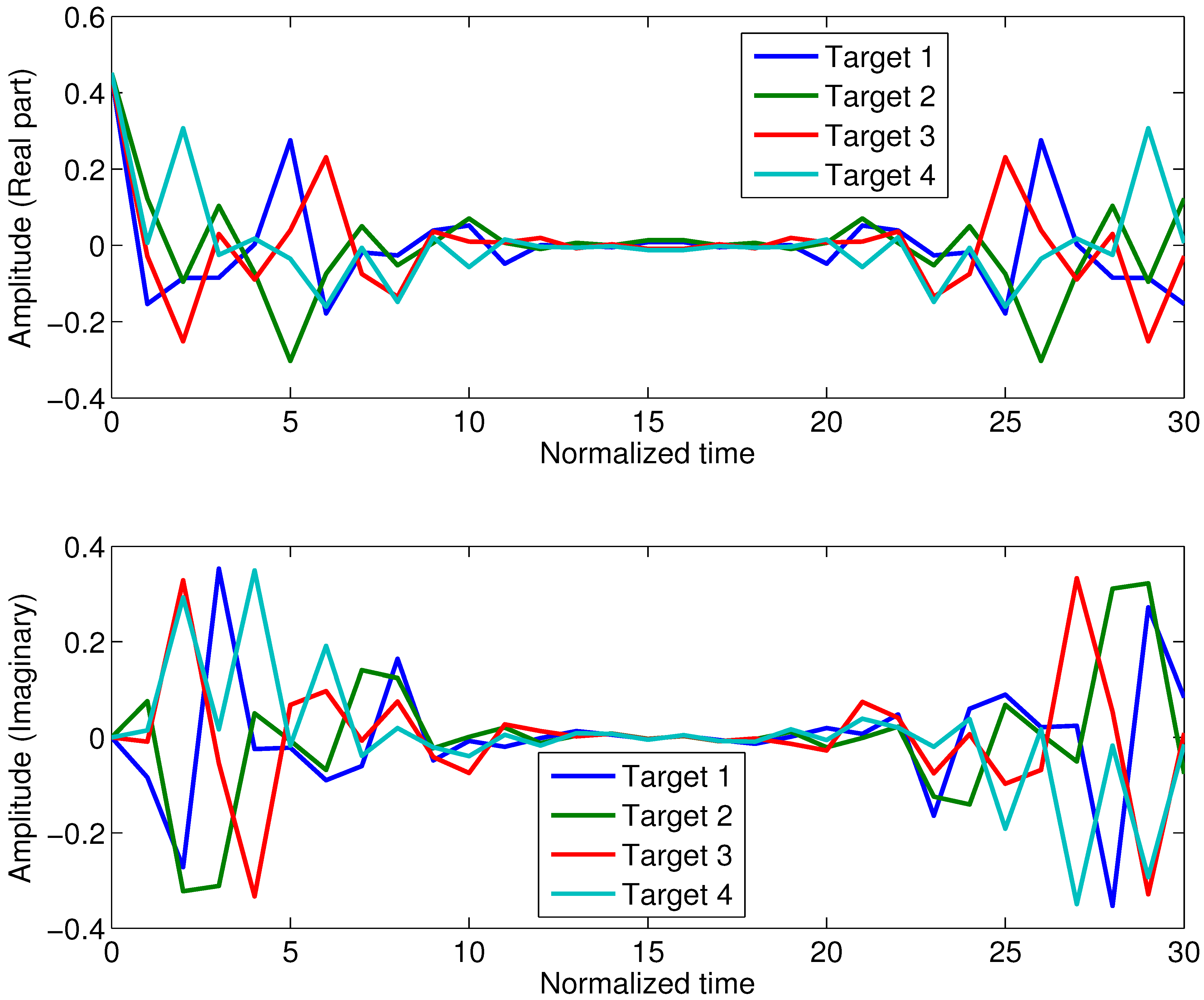
3.1. Matched Waveform to a Target Response

For convenience, we use the discrete-time model, where the sampling instant is normalized, such that T s = 1 . It is sufficient to illustrate both types of CRr by using a deterministic target response. This is because the CRr can be extended for various target types (deterministic or stochastic) by consulting [16]. Our focus here is not on target types, but rather on CRr types. First, we review the notion of a transmit waveform matched to an extended target response. If a target has a known response, it turns out that there is such a waveform that maximizes the received signal energy or power out of a matched filter receiver given a transmit energy constraint [19]. In other words, this waveform also maximizes the received signal-to-noise ratio (SNR).
Let h be the complex-valued target response, and let x be an arbitrary complex-valued transmit waveform. Let the complex-valued vector w be the additive white Gaussian noise from the receiver hardware. Thus, the received signal plus noise is y = s + w where s = h * x , and (*) designates the convolution operation. For convenience, we can specifically describe h = E h h ¯ , such that E h is the target response energy and h ¯ is a unit energy vector. It follows that we can let x = E x x ¯ , such that E x is the transmit waveform energy and x ¯ is a unit energy vector. Then, y = E h h ¯ * E x x ¯ + w . If we let H ¯ be the target response convolution matrix [14], then:
y = E h E x H ¯ x ¯ + w
where w being a complex-valued white Gaussian noise process has a covariance matrix given by σ 2 I . We recall that σ 2 is the variance of one noise sample. Using the proper matched filter to the received signal plus noise, i.e., ( H x ) y , then the received energy due to the echo s = h * x is given by:
E s = E x E h H ¯ x ¯ H ¯ x ¯ = E x E h x ¯ H ¯ H ¯ x ¯
where † represents the conjugate-transpose or Hermitian operation. If we let R ¯ = H ¯ H ¯ be the autocorrelation of the target convolution matrix, then the received energy due to the target echo for any transmit waveform is given by:
E s = E h E x x ¯ R ¯ x ¯
Using eigenvalue decomposition, we realize
E s , λ = E h E x q ¯ λ q ¯ = E h E x λ
where E s , λ corresponds to a particular eigenvalue λ and its corresponding unit-energy eigenvector q ¯ . Thus, we can maximize the received energy E s by choosing the eigenvector corresponding to the maximum eigenvalue to be our transmit waveform. Thus, the maximum received echo energy is given by:
E s , max = E h E x λ max q ¯ max q ¯ max = E h E x λ max
where the matched transmit waveform that maximizes the received echo energy is clearly x = E x q ¯ max , i.e., x ¯ = q ¯ max , which is sometimes referred to as the eigen-waveform.

3.2. Multiple Hypothesis Testing

While it is useful to know that an eigen-waveform exists for a specific target response, our goal in this work is to determine which target is present from among M known alternatives (deterministic responses). Again, extension to stochastic targets is straightforward via [15,16]. There are M hypotheses for the target channel, and each hypothesis is characterized by a target response and a prior probability of that hypothesis being true. Our goal is to identify the correct hypothesis as accurately as possible with a single or multiple energy-limited transmissions. We will assume equal prior probabilities for each target (initially when no transmission has been sent), but we show how other priors can be incorporated. A Bayesian representation of the channel is formulated where the target hypotheses are denoted by H 1 , H 2 , ..., H M with corresponding prior probabilities P 1 , P 1 , ..., and P M . The i-th hypothesis is characterized by a target response s i with corresponding target convolution matrix H ¯ i , i = 1, 2, ..., M.
The recognition or identification hypotheses are:
H 1 : y = s 1 + w = E h H ¯ 1 E x x ¯ + w H 2 : y = s 2 + w = E h H ¯ 2 E x x ¯ + w H M : y = s M + w = E h H ¯ M E x x ¯ + w
With w C N ( 0 , σ 2 I ) , the corresponding pdfs are given by:
p ( y | H 1 ) = 1 π N σ 2 N exp - 1 σ 2 ( y - s 1 ) ( y - s 1 ) p ( y | H 2 ) = 1 π N σ 2 N exp - 1 σ 2 ( y - s 2 ) ( y - s 2 ) p ( y | H M ) = 1 π N σ 2 N exp - 1 σ 2 ( y - s M ) ( y - s M )
where N is the length of the received measurement.

3.3. Transmit Adaptive Waveform

In the multiple hypothesis testing (MHT) identification problem described above, the radar tries to figure out which target is present among the target alternatives. In other words, we cannot simply use one of the eigen-waveforms since we do not know which target is present a priori. Various adaptive waveforms were used in our previous works [14,15,16], and most of them performed well compared to simply using a (non-adaptive) pulsed wideband waveform. It was difficult to ascertain which specific waveform performed the best, both in terms of ANI or P c d , since some waveforms performed well in high SNR, but not necessarily low SNR, while others performed well in low SNR and not necessarily high SNR. Furthermore, a waveform scheme may perform well in terms of P c d , but not necessarily ANI. In this work, it would be best to find a waveform that consistently performs well, both in terms of P c d and ANI for all transmit energy constraints. As such, we will propose one. When the target alternatives have stochastic responses, a particular proposed adaptive waveform is based on scaling each eigen-waveform matched to each target alternative and summing them while meeting the transmit energy constraint [18]. This waveform was called the probability weighted (PWE) SNR-based waveform since the scaling used is based on the prior (or updated) probabilities of the the hypotheses corresponding to the target alternatives. In [18], preliminary results suggest that the PWE-SNR waveform performs consistently well in terms of P c d against the wideband waveform for all transmit energy constraints. However, it was not addressed in that paper how the PWE-SNR waveform would perform in terms of ANI, which we need to accomplish our goal of comparing the two radar platforms. Thus, we have extended our simulations and shown that it also performed well in terms of ANI vs. the wideband waveform for all of the transmit energy levels. As such, we will use this waveform in comparing how SHT-CRr and MAP-CRr perform. Initially, the waveform is formed via:
x t = m = 1 M P m q ¯ m
where q ¯ m corresponds to the unit-energy eigen-waveform corresponding the m-th target hypothesis, and P m corresponds to the initial probability. Since the energy in Equation (8) may not result to unity, we can meet the transmit energy constraint by:
x = E x x t E x t
where E x t is the resulting energy of the non-unit energy waveform, while the scaling E x ensures that the transmit energy constraint is met.

3.4. Probability Updating

One of the components that makes a radar cognitive is its ability to extract or use knowledge from previous received measurements. For the CRr mentioned in our previous works, this comes in the form of the updated probabilities for all of the target hypotheses via the Bayesian framework. In other words, the updated probability after first transmission for any of the hypothesis in Equation (7) is given by:
P m , 1 = p ( y 1 | H m ) p ( y ) P m
where the “1” in P m , 1 signifies the updated probability after the first transmission is received and processed by the receiver. By virtue of total probability, the sum of the updated probabilities is one, and thus, the denominator in Equation (10) may be replaced by a scaling that ensures that the sum leads to one. In other words, the updated probability for any number of transmission k + 1 is given by:
P m , k + 1 = β p ( y k + 1 | H m ) P m , k
where β ensures unit total probability. Note that the updated probability in Equation (11) is dependent on the latest measurement y k + 1 , as it should be. However, it is also dependent on the prior update P m , k , which was dependent on prior measurement y k . In other words, the prior probability update information is kept and still used in the latest probability update.
Thus, the next ( k + 2 ) -th transmit waveform is given by:
x t = m = 1 M P m , k + 1 q ¯ m
where Equation (9) is needed to meet the transmit energy constraint.

3.5. MAP-CRr and SHT-CRr
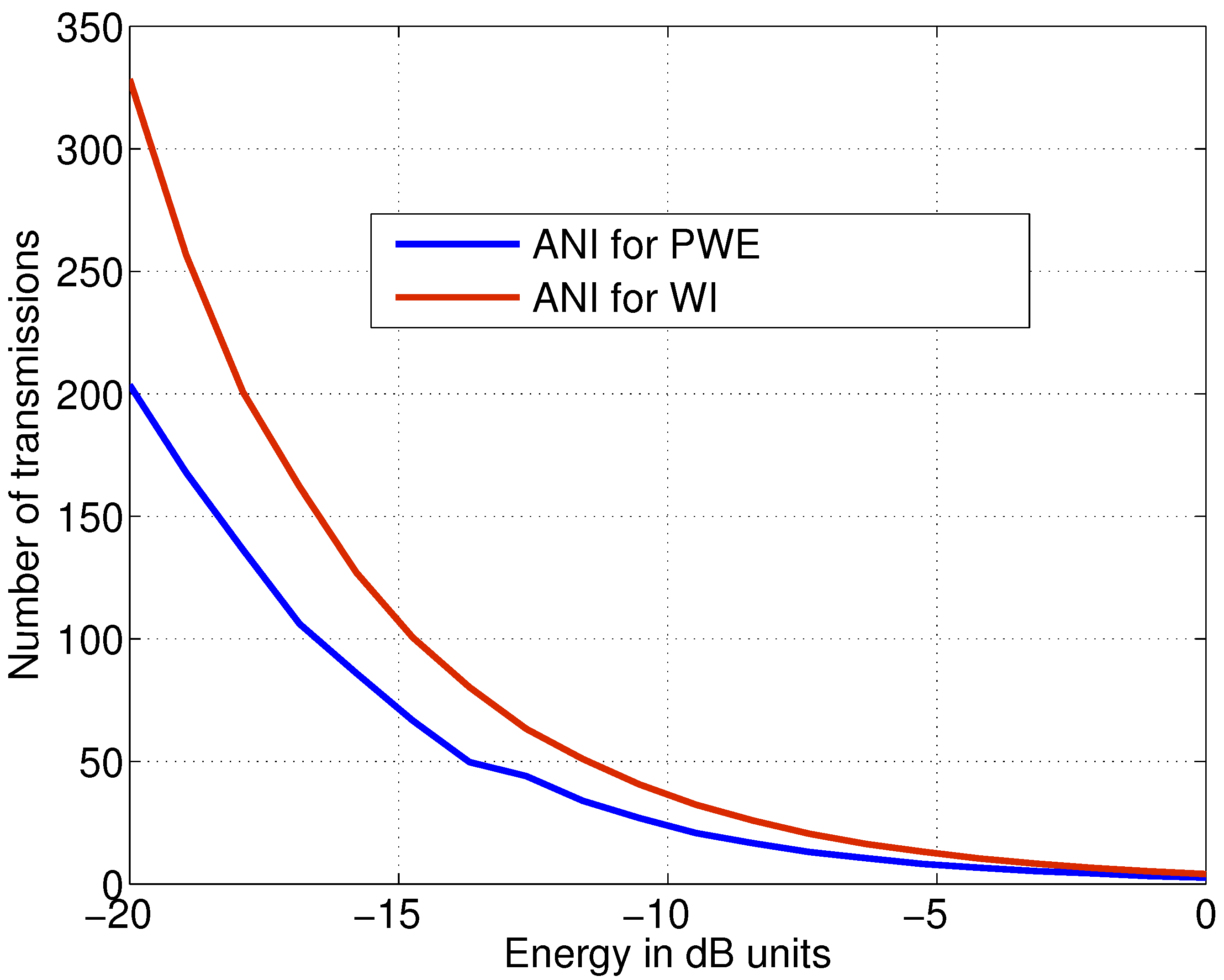
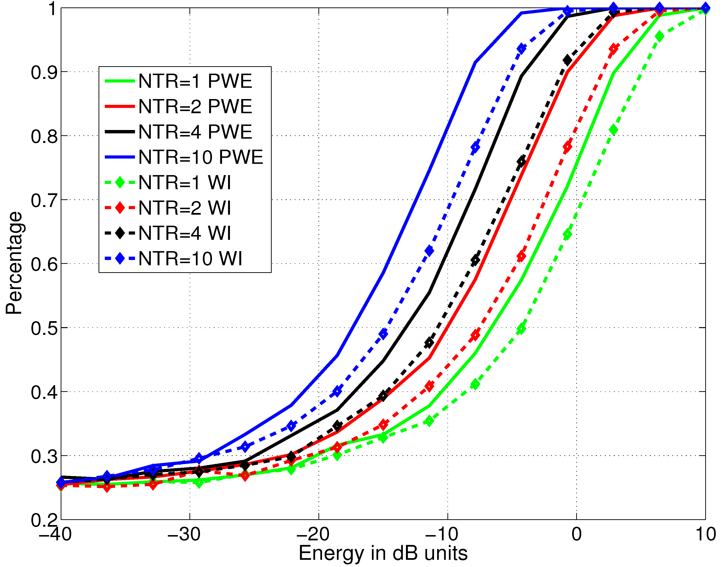
Looking at Figure 1, we finally arrive at a point where we can differentiate MAP-CRr and SHT-CRr in terms of how to terminate transmission and deciding which target is present. The MAP-CRr is used when the number of transmissions is constrained. For example, if the number of transmission is constrained to k + 1 , then the previously-updated probabilities are again updated after the processing of ( k + 1 ) -th received signal as dictated by Equation (11). Then, the radar makes a decision. To make a decision, the receiver looks at all of the latest probabilities and notes the one with the highest update. The receiver decides that the target present (whether true or not) corresponds to the hypothesis with that highest update, which leads to the name MAP-CRr.
Another way to operate a CRr is to not constrain the number of transmissions. To decide if a target is present, the CR uses a probability threshold, which when met by one of the updated hypothesis probabilities, triggers the CR to stop transmission. For example, a probability threshold desired could be 0.9, and the radar does not stop transmission until this threshold is crossed by one of the updated probabilities via Equation (11), as shown in Figure 1. The radar decides that the hypothesis whose probability crosses the threshold is the target present (whether true or not). We name this radar SHT-CRr.

4. P c d and ANI

Our focus here is not to design more adaptive waveform schemes. As mentioned before, our goal is to compare the two types of cognitive radar used for target identification. In order to compare SHT-CRr and MAP-CRr, we do need to use some waveforms for the purposes of illuminating the target scene. As mentioned before, we will use the SNR-PWE waveform, as well as the wideband waveform (to ensure that the SNR-PWE waveform consistently outperforms the wideband waveform in terms of P c d and ANI for all transmit energy levels).
Let us briefly describe the CRr simulation setup that will produce the P c d and ANI that we need for CRr comparison. We set up a target recognition experiment where we assume that a deterministic extended target is present from four known alternatives, i.e., M = 4 . For the sake of completeness, such that this research can be reproduced by an interested reader, we include the four target responses used in our experiments. Although not necessary, the target responses were generated to have unit energy. Recall that our targets are complex valued, and thus, the real and imaginary responses are shown in Figure 2. Various target responses can be used in the Monte Carlo experiment. Here, the targets were generated such that they are resonant in certain frequency bands (to simulate extended targets exhibiting such properties). The corresponding magnitude spectra for these targets are shown in Figure 3, which shows the resonant nature of these targets.
Figure 2. Extended target responses used in the Monte Carlo target identification experiments (real and imaginary portions).
Aerospace 02 00376 g002
Figure 3. Magnitude spectra of the four target responses showing resonant bands.
Aerospace 02 00376 g003
The CRr forms the PWE-SNR waveform by scaling the four SNR-based waveforms (also known as eigen-waveforms) matched to those four targets. The scaling is a function of the four prior probabilities as dictated by Equations (10)–(12). The waveform-target convolution echo is added to Gaussian noise in the receiver. The measurement is processed and used to update the prior probabilities via Bayes theorem Equation (10). For the SHT-CRr, if the probability threshold is not met, then a new PWE-SNR waveform is adaptively designed as dictated by Equations (8) and (9) and transmitted. For MAP-CRr, if the number of transmission thresholds is not exceeded, then the transmission continues with a new waveform, as dictated by Equations (8) and (9). For the results shown in this paper, each ANI or P c d curve is a result of 100,000 Monte Carlo trials where a target is randomly chosen from the alternatives. First, let us look at the performance of both the PWE-SNR waveform and the pulsed wideband waveform in terms of ANI. In Figure 4, we show the resulting ANI vs. transmit energy for the PWE-SNR and wideband waveforms with SHT-CRr using a probability threshold of 0.90. Notice that the PWE-SNR (labeled “PWE”) waveform outperforms the wideband (labeled “WI”) for all transmit energy values. In other words, the ANI needed to support the 0.90 probability threshold is smaller for the PWE than the wideband waveform. In all of our various experiments, the PWE waveform consistently performed better than wideband for all ranges of transmit energy in terms of ANI for various probability thresholds used. For brevity, we only include results using a probability threshold of 0.90 here, since we will use these particular results when we finally compare SHT-CRr and MAP-CRr, which is the main objective of this paper.
With the same simulation set (using MAP-CRr this time), we show the resulting P c d vs. transmit energy with various numbers of transmissions in Figure 5 for PWE and wideband waveforms. Notice that the PWE waveform consistently outperforms the wideband waveform for all ranges of energy given a fixed number of transmissions (labeled “NTR”).
Figure 4. Average number of illuminations (ANI) vs. transmit energy in dB units with SHT-CRr using probability weighted energy (PWE)-SNR (labeled “PWE” and wideband (labeled “WI”) waveforms.
Aerospace 02 00376 g004
Figure 5. P c d vs. transmit energy in dB units for various numbers of transmissions (labeled “NTR”) with MAP-CRr using PWE-SNR (labeled “PWE”) and wideband (labeled “WI”) waveforms.
Aerospace 02 00376 g005

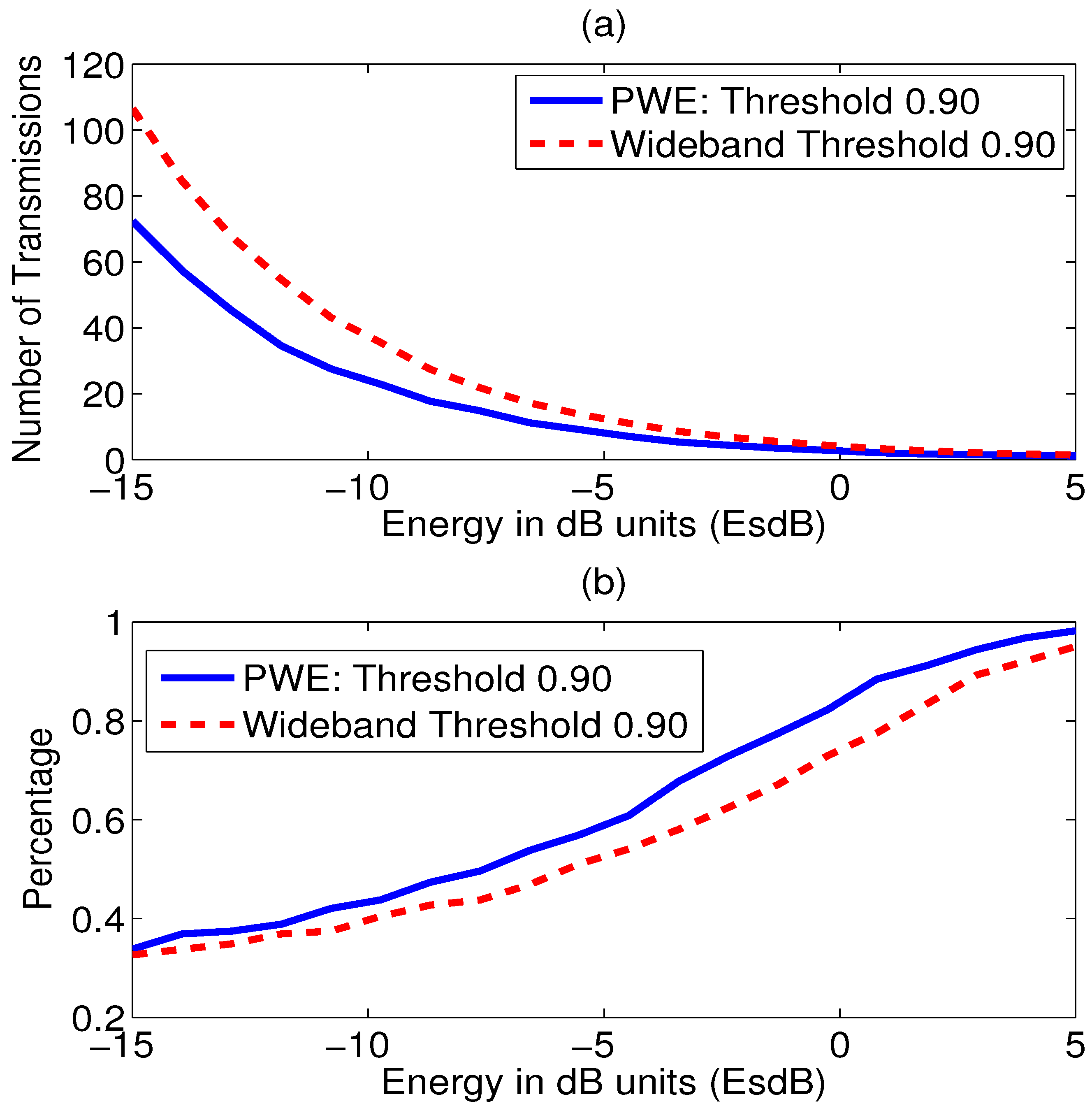
5. Comparing Total Transmit Energy

For SHT-CRr, it would seem that if we calculate the P c d of a Monte Carlo trial that it would be close if not equal to the probability threshold used. After all, this is the reason why a probability threshold would be used. While we were aware that that the probability threshold may have been different from the eventual P c d , this fact was never explored from our previous works [12,13,14,16]. We found out in this work that the probability threshold could be drastically different from the eventual P c d . This is because in an experiment, while SHT-CRr does ensure that transmission stops when the probability update threshold is met, it does not mean a correct decision is made. In other words, while the updated probability of one of the target hypotheses may actually cross the probability threshold, it does not necessarily mean that the target present in the actual experiment corresponds to that hypothesis. It turns out that the discrepancy is a function of the transmit energy. Indeed, the P c d for the experiment corresponding to the results in Figure 4 is shown in Figure 6b, while we repeat Figure 4 in Figure 6a for convenience. We notice that the P c d increases (and not a constant, like the 0.90 probability threshold) as a function of increasing transmit energy. Conversely, the lower the transmit energy is, the lower is the P c d despite the fact that the ANI is higher. This is important to recognize. In other words, limiting the transmit energy used per pulse and simultaneously allowing the number of transmissions to be non-limited does not actually increase the P c d , which is a profound observation (at least for the two waveforms used here and the various various waveforms we tested so far). It is not until high transmit energy is used (here, between 0 and 5 dB energy units) that both PWE-SNR and wideband waveforms actually meet the 0.90 probability threshold. This is a critical and important result for system designers to realize.
Recall that SHT-CRr and MAP-CRr clearly have different metrics in terms of performance (ANI and P c d for MAP-CRr). Thus, in order to compare SHT-CRr and MAP-CRr, we have to formulate a metric that effectively multiplies the number of transmissions or ANI to transmit energy level (per pulse) to produce a metric called total transmit energy (TTE) for a given P c d . We mentioned that fixing a P c d is difficult to implement in the simulation. Therefore, we recall the procedure discussed in Section 2 that allows us to perform the comparison. We will use both the PWE-SNR and wideband waveforms to illustrate the comparison.

5.1. Comparison with the PWE Waveform

From Figure 6, we see that at - 15 dB energy units (low energy case), ANI 73 . 4 and P c d 0 . 34 using SHT-CRr. With NTR = 2 at - 15 dB energy units in Figure 5 using MAP-CRr, P c d 0 . 39 . In other words, the same performance is easily met by MAP-CRr by limiting the transmissions to a fixed number of two (instead of an ANI of 73.4). Since we defined TTE to be the number of transmissions times transmit energy, then for SHT-CRr to meet P c d 0 . 34 , TTE = 3.7 dB energy is needed. Using MAP-CRr with NTR = 2, then TTE = - 12 dB energy (which is a difference of 15.7 dB), which means MAP-CRr is more efficient in using energy than SHT-CRr (with threshold 0.90) at low transmit energies. At - 5 dB energy units (medium energy), ANI 8 . 0 and P c d 0 . 59 using SHT-CRr. With NTR = 2 at - 5 dB energy using MAP-CRr, P c d = 0 . 74 (Figure 5). Thus, the the performance is again exceeded by MAP-CRr by limiting the transmissions to two. Using SHT-CRr, TTE = 4 dB energy units, and using MAP-CRr, TTE = - 2 dB units for a difference of 6 dB. In other words, the performance difference begins to lessen as transmit energy is increased. At 5 dB of energy units (large energy), ANI 1 . 15 and P c d 0 . 98 using SHT-CRr. In other words, it only takes a little over one transmission on average to get a P c d that is close one. With NTR = 1 at 5 dB energy units using MAP-CRr, the P c d 0 . 96 . The TTE is slightly higher for SHT-CRr, but SHT-CRr has a slightly better P c d in this high energy case. The TTE and P c d differences are very small, enforcing the observation that performance difference between two platforms lessens as a function of increasing transmit energy.
Figure 6. (a) ANI vs. transmit energy ( E s ) in dB ( E s dB) for PWE and wideband waveforms and (b) P c d vs. transmit energy ( E s ) in dB (EsdB) for PWE and wideband waveforms using a probability threshold of 0.90 with the SHT-CRr platform.
Aerospace 02 00376 g006

5.2. Comparison with the Wideband Waveform

Mirroring the analysis above, from Figure 6, we see that at - 15 dB energy units (low energy case), ANI 106 . 5 and P c d 0 . 33 using SHT-CRr with the wideband waveform labeled “WI”. With NTR = 2 at - 15 dB energy units in Figure 5 using MAP-CRr, P c d 0 . 33 . In other words, the same performance is easily met by MAP-CRr by limiting the transmissions to a fixed number of two (instead of an ANI of 106.5). Thus, the total effective energy for SHT-CRr to meet P c d 0 . 33 is TTE = 5.5 dB energy (this is more than the 3.7 dB needed for the PWE waveform, as expected, since PWE actually changes waveform every illumination, making for a true feedback system). As before with MAP-CRr with NTR = 2, then TTE = - 12 dB energy (which is a difference of 17.5 dB), which again shows that MAP-CRr is more efficient at using energy than SHT-CRr (using threshold 0.90) at low transmit energies. At - 5 dB energy units (medium energy), ANI 12 . 0 , and P c d 0 . 52 using SHT-CRr. With NTR = 4 at - 5 dB energy using MAP-CRr, P c d = 0 . 6 . Thus, the the performance is again exceeded by MAP-CRr by limiting the transmissions to four instead of ANI of twelve. Using SHT-CRr, TTE = 3.8 dB energy units, and using MAP-CRr, TTE = 1 dB unit, for a difference of 2.8 dB. Just like what is observed with the PWE waveform, the performance difference begins to lessen as transmit energy is increased. At 5 dB of energy units (large energy), ANI 1 . 42 and P c d 0 . 95 using SHT-CRr. In other words, it only takes a little over one transmission on average to get a P c d of 0.95. Again, since this is a non-adaptive waveform, its P c d performance is lower than that of PWE, which is close to one. With NTR = 1 at 5 dB energy units using MAP-CRr, the P c d 0 . 95 , which illustrates that MAP-CRr TTE is just slightly lower than SHR-CRr TTE. In other words, even with the use of the wideband waveform, it is clear that from very low to high energy transmission, the effective transmit energy is better for MAP-CRr than SHT-CRr, which makes it more efficient.
It should be mentioned that we also used other reasonable probability thresholds (e.g., 0.95) in our Monte Carlo experiments. In the interest of brevity, we do report that the TTE is better for MAP-CRr than SHT-CRr for both waveforms, which lessens as transmit energy is increased. In other words, the same conclusions are observed despite changing the probability threshold.

6. Conclusions

In this paper, we set out to compare two CRr platforms for target recognition, called SHT-CRr and MAP-CRr, in terms of transmit energy efficiency. A direct comparison was difficult, since the performance metrics are different: ANI for SHT-CRr and P c d for MAP-CRr. In target identification, however, the probability of correct classification is one of the utmost requirements. Thus, we looked at the eventual SHT-CRr P c d . We reported that the P c d performance of SHT-CRr could be drastically different from the probability threshold used.
We proposed a procedure for how to compare the two radars. The procedure basically tries to find comparable P c d ’s from both radar Monte Carlo results. We find two P c d ’s that are as close as possible. Then, we compare the metric called total transmit energy for those P c d ’s. Since the transmissions are multiple, TTE is the total effective energy used. We needed a waveform that consistently outperforms the wideband waveform in terms of P c d and ANI for all possible transmit energy levels. We showed that a waveform called the PWE-SNR waveform outperforms the wideband waveform in terms of ANI and P c d for all ranges of transmit waveform energy. We used both (PWE-SNR and wideband) waveforms to facilitate the comparison of SHT-CRr and MAP-CRr. It is shown that at very low to high transmit energy, the TTE for MAP-CRr is better than SHT-CRr (which means more energy efficiency), but the efficiency difference lessens as the transmit energy is increased.

Author Contributions

Dr. Ric Romero authored this article. The paper was based off the Master’s thesis work (in Electrical Engineering) by his student LT Emmanouil Mourtzakis of the Hellenic Navy at the Naval Postgraduate School in Monterey, CA.

Conflicts of Interest

The authors declare no conflict of interest.

References

  1. US Department of the Air Force. Air Navigation; Department of the Air Force: Washington, DC, USA, 2001. [Google Scholar]
  2. Bowditch, N. The American Practical Navigator; National Imagery and Mapping Agency: Bethesda, MD, USA, 2002. [Google Scholar]
  3. Crippen, D. The air traffic control radar beacon system. IRE Trans. Aeronaut. Navig. Electron. 1957, ANE-4, 6–15. [Google Scholar] [CrossRef]
  4. Federal Aviation Administration. Air Traffic 101. Available online: http://www.faa.gov (accessed on 24 March 2015).
  5. Stimson, G. Introduction to Airborne Radar; SciTech Publishing: Mendham, NJ, USA, 1998. [Google Scholar]
  6. Kovaly, J.J. Synthetic Aperture Radar; Artech House: Norwood, MA, USA, 1978. [Google Scholar]
  7. Currie, A. Synthetic aperture radar. IET Electron. Commun. Eng. J. 1957, 3, 159–170. [Google Scholar] [CrossRef]
  8. Essen, H.; Makaruschka, R. Remote sensing of land and water with an airborne 94 GHz synthetic aperture radar. In Proceedings of the 25th European Microwave Conference, Bologna, Italy, 4 September 1995; pp. 567–570.
  9. Ulaby, F. Microwave Radar and Radiometric Remote Sensing; University of Michigan Press: Ann Arbor, MI, USA, 2013. [Google Scholar]
  10. Fuhrmann, D. Active-testing surveillance systems, or, playing twenty questions with a radar. In Proceedings of the 11th Annual Adaptive Sensor and Array Processing (ASAP) Workshop, Lexington, MA, USA, 11–13 March 2003.
  11. Haykin, S. Cognitive radar: A way of the future. IEEE Signal Process. Mag. 2006, 23, 30–40. [Google Scholar] [CrossRef]
  12. Guerci, J.R. Cognitive Radar: The Knowledge-Aided Fully Adaptive Approach; Artech House: Norwood, MA, USA, 2010. [Google Scholar]
  13. Aubry, A.; DeMaio, A.; Farina, A.; Wicks, M. Knowledge-aided (potentially cognitive) transmit signal and receive filter design in signal-dependent clutter. IEEE Trans. Aerosp. Electron. Syst. 2013, 49, 93–117. [Google Scholar] [CrossRef]
  14. Goodman, N.; Venkata, P.; Neifeld, M. Adaptive waveform design and sequential hypothesis testing for target recognition with active sensors. IEEE J. Sel. Top. Sig. Proc. Mag. 2007, 1, 105–113. [Google Scholar] [CrossRef]
  15. Hyeong-Bae, J.; Goodman, N. Adaptive waveforms for target class discrimination. In Proceedings of the 2007 Waveform Diversity and Design Conference, Pisa, Italy, 4–8 June 2007; pp. 395–399.
  16. Romero, R.; Goodman, N. Waveform design in signal-dependent interference and application to target recognition with multiple transmissions. IET Radar Sonar Navig. 2009, 3, 328–340. [Google Scholar] [CrossRef]
  17. Romero, R.; Bae, J.; Goodman, N. Theory and application of SNR and mutual information matched illumination waveforms. IEEE Trans. Aerosp. Electron. Syst. 2011, 47, 912–926. [Google Scholar] [CrossRef]
  18. Romero, R.; Goodman, N. Improved waveform design for target recognition with multiple transmissions. In Proceedings of the IEEE International Waveform Diversity and Design Conference, Orlando, FL, USA, 8–13 February 2009.
  19. Bell, M. Information theory and radar waveform design. IEEE Trans. Inform. Theory 1993, 39, 1578–1597. [Google Scholar] [CrossRef]

