An Efficiently Parallelized High-Order Aeroacoustics Solver Using a Characteristic-Based Multi-Block Interface Treatment and Optimized Compact Finite Differencing

Abstract

This paper presents the development of a fourth-order finite difference computational aeroacoustics solver. The solver works with a structured multi-block grid domain strategy, and it has been parallelized efficiently by using an interface treatment based on the method of characteristics. More importantly, it extends the characteristic boundary condition developments of previous researchers by introducing a characteristic-based treatment at the multi-block interfaces. In addition, most characteristic methods do not satisfy Pfaff’s condition, which is a requirement for any mathematical relation to be valid. A mathematically-consistent and valid method is used in this work to derive the characteristic interface conditions. Furthermore, a robust and efficient approach for the matching of turbulence quantities at the multi-block interfaces is developed. Finally, the implementation of grid metric relations to minimise grid-induced errors has been adopted. The code was validated against a number of benchmark cases, which demonstrated its accuracy and robustness across a range of problem types.

1. Introduction

Aerodynamically-generated noise is an often undesirable by-product of unsteady fluid motion. From ground vehicles (road vehicles, high-speed trains) to commercial and military aircraft, unwanted aerodynamic noise generation imposes significant problems. In aerospace applications, the noise generated by separated shear layers and vortex shedding can induce vibration leading to fatigue failure of the structure. Undercarriage, weapons bays, high-lift devices, excrescences and turbomachinery are just some examples of noise sources. To address these issues, a detailed understanding of the nature of the source responsible, the noise generation mechanisms and the noise radiation characteristics is required. Hence, a computational solver that is capable of accurately modelling the responsible flow physics is desirable. A numerical simulation of noise problems must resolve both the source evolution and sound propagation phenomena accurately enough so that sound fields are not contaminated by numerical errors. To avoid the accumulation of errors in wave propagation problems, numerical schemes are required, therefore to have low dissipation and dispersion. The minimisation of errors has been the main challenge in aeroacoustics since computational methods were first employed. When the acoustic waves are part of the source mechanisms, as in cases involving acoustic and flow feedback, Singer and Guo [1] found numerical dispersion to be the most harmful because it corrupts the phase information of the waves affecting the interaction between flow and sound.

The numerical modelling of aeroacoustic phenomena is demanding for several reasons [2]. Foremost is the fact that aeroacoustic problems are, by definition, time dependent. They must, therefore, be treated time-accurately with appropriate consideration of all relevant scales. Since the human ear is sensitive to a wide range of frequencies, typically 20 Hz to 20 kHz, simulations dealing with such problems must also span this broad spectrum. An equally important consideration is the disparity between the energy levels of the unsteady flow fluctuations and the acoustic signals. A fairly intense acoustic wave of 100 dB contains pressure fluctuations that are three orders of magnitude smaller than those in a typical turbulent flow. There are also large differences in the length scale present between the acoustic variables and the flow variables, i.e., the turbulent length scale is much larger than the acoustic one. The emergence of computational aeroacoustics (CAA) as a viable research tool is a testament, not only to the proliferation of powerful computer resources, but also the development and improvement of high-order accurate schemes, available in a variety of forms. Both explicit and implicit finite difference spatial discretization schemes are widely used [3,4,5]. Explicit schemes employ large computational stencils for accuracy, whereas implicit schemes achieve high-order accuracy by solving for the spatial derivatives implicitly using relatively compact stencils.

One major issue with any high-order solver is the sensitivity of the solution to the grid skewness and the boundary conditions used. It is desirable, therefore, to have a boundary formulation that avoids any kind of extrapolation or simplification while solving the governing equations at the boundary. Boundary conditions based on the method of characteristics have been developed to meet these high accuracy requirements and have been continuously evolving for many years [6,7,8,9,10]. Characteristic boundary conditions for Navier–Stokes equations (NSCBC) are widely used, for example, in reacting flows and high temperature mixtures [11,12,13]. Another important advantage of this method is that it can be used to efficiently parallelize the solver in multi-block domains because it avoids the excessive communication at multi-block interfaces required by other inter-block treatments, for example overlapping grids. Hence, characteristic-based methods have started to find use to treat the block interfaces in multi-block grid domains for efficient parallel computations [14,15]. However, these methods are only valid for inviscid and laminar flows. There is also a mathematical consistency issue which exists for multi-dimensional Navier–Stokes equations, when characteristic equations are expressed in the form given in the literature [9,14,15,16]. As previously stated by Chen and Zha [17] when referring to the work of Kim and Lee [9], the characteristic equations in this form do not satisfy Pfaff’s condition and “…it is incorrect to express the characteristic form of the Navier–Stokes equations in the form given in (Kim and Lee [9]).”.

Pfaff’s condition is a mathematical requirement, which needs to be satisfied by any differential equations, and its importance was first demonstrated by Thompson [6] while deriving characteristic boundary conditions. Chen and Zha [17] were the first to derive the characteristic boundary conditions that satisfied Pfaff’s condition for generalized meshes. In their form, however, it is only applicable to inflow and outflow boundaries. One of the aims of this paper was to extend the work of Chen and Zha [17] to derive the multi-block grid interface matching using the method of characteristics.

In addition, all of the existing interface treatments based on the method of characteristics lack a satisfactory interface matching of turbulence quantities. To address these issues, the mathematically-consistent form of the characteristic equations relevant to interface treatment were derived. The proposed method has been implemented in a fourth-order computational aeroacoustic (CAA) solver that works with structured multi-block grid domains. Adaptation of the interface treatment avoids using the computationally-expensive grid stencils swapping at the inter-block interface, which in turn, significantly reduces the computation burden of parallelization. In addition, the work presented here outlines the implementation of metric cancellation errors to extend the use of the CAA code to complex geometries with curvilinear grids.

2. Fourth-Order Solver

The fourth-order solver uses a compact finite-differencing approach to evaluate the first-order spatial derivatives in the conservative form of the governing equations and a delayed detached-eddy simulation (DDES) approach to turbulence modelling. The finite difference method allows the formulation of accurate high-order schemes relatively easily because the high-order accuracy can be maintained for complex geometries through the use of a curvilinear coordinate system. Specifically, a fourth-order pentadiagonal type of central compact finite-difference scheme in space and fourth-order explicit temporal differencing are used to minimise the dissipation and dispersion errors. The solver is parallelised using the Message-Passing Interface (MPI) library, which establishes efficient communication between the individual computing cores within the parallel computing cluster.

2.1. Governing Equations

The time-dependent, three-dimensional Navier–Stokes equations can be expressed, in Cartesian coordinates as,

$$\frac{\partial \mathbf{Q}}{\partial t}+\frac{\partial \mathbf{E}}{\partial x}+\frac{\partial \mathbf{F}}{\partial y}+\frac{\partial \mathbf{G}}{\partial z}={\mathbf{S}}_v$$

(1)

where the conservative variables and the inviscid flux variables are represented as:

$$\mathbf{Q}=\left[\begin{array}{c}\rho \\ \rho u\\ \rho v\\ \rho w\\ \rho e_t\end{array}\right],\mathbf{E}=\left[\begin{array}{c}\rho u\\ \rho u^2+p\\ \rho uv\\ \rho uw\\ (\rho e_t+p)u\end{array}\right],\mathbf{F}=\left[\begin{array}{c}\rho v\\ \rho uv\\ \rho v^2+p\\ \rho vw\\ (\rho e_t+p)v\end{array}\right],\mathbf{G}=\left[\begin{array}{c}\rho w\\ \rho uw\\ \rho vw\\ \rho w^2+p\\ (\rho e_t+p)w\end{array}\right]$$

(2)

For air as an ideal gas, the total energy term is given by $\rho e_t=p/\left(\gamma -1\right)+0.5\rho \left(u^2+v^2+w^2\right)$, where $\gamma =c_p/c_v$ is the ratio of specific heat coefficients under constant pressure and constant volume. The right-hand term, ${\mathbf{S}}_v$, in Equation (1) is the source term containing the viscous flux derivatives and is represented as,

$${\mathbf{S}}_v=\frac{\partial {\mathbf{E}}_v}{\partial x}+\frac{\partial {\mathbf{F}}_v}{\partial y}+\frac{\partial {\mathbf{G}}_v}{\partial z}$$

(3)

where,

$$\begin{array}{cc}\hfill {\mathbf{E}}_v=\left[\begin{array}{c}0\\ {\tau }_{xx}\\ {\tau }_{xy}\\ {\tau }_{xz}\\ u{\tau }_{xx}+v{\tau }_{xy}+w{\tau }_{xz}+q_x\end{array}\right],& {\mathbf{F}}_v=\left[\begin{array}{c}0\\ {\tau }_{yx}\\ {\tau }_{yy}\\ {\tau }_{yz}\\ u{\tau }_{yx}+v{\tau }_{yy}+w{\tau }_{yz}+q_y\end{array}\right],\hfill \\ & {\mathbf{G}}_v=\left[\begin{array}{c}0\\ {\tau }_{zx}\\ {\tau }_{zy}\\ {\tau }_{zz}\\ u{\tau }_{zx}+v{\tau }_{zy}+w{\tau }_{zz}+q_z\end{array}\right]\hfill \end{array}$$

(4)

The viscous stress tensor components are related to the Cartesian velocity components by the following equations.

$$\begin{array}{cccc}\hfill {\tau }_{xx}& =\frac{1}{{\mathrm{Re}}_{\infty }}\left(2{\mu }_{\mathrm{eff}}\frac{\partial u}{\partial x}+\lambda \nabla ·\mathbf{v}\right),\hfill & \hfill {\tau }_{xy}& ={\tau }_{yx}=\frac{{\mu }_{\mathrm{eff}}}{{\mathrm{Re}}_{\infty }}\left(\frac{\partial u}{\partial y}+\frac{\partial v}{\partial x}\right),\hfill \\ \hfill {\tau }_{yy}& =\frac{1}{{\mathrm{Re}}_{\infty }}\left(2{\mu }_{\mathrm{eff}}\frac{\partial v}{\partial y}+\lambda \nabla ·\mathbf{v}\right),\hfill & \hfill {\tau }_{yz}& ={\tau }_{zy}=\frac{{\mu }_{\mathrm{eff}}}{{\mathrm{Re}}_{\infty }}\left(\frac{\partial v}{\partial z}+\frac{\partial w}{\partial y}\right),\hfill \\ \hfill {\tau }_{zz}& =\frac{1}{{\mathrm{Re}}_{\infty }}\left(2{\mu }_{\mathrm{eff}}\frac{\partial w}{\partial z}+\lambda \nabla ·\mathbf{v}\right),\hfill & \hfill {\tau }_{xz}& ={\tau }_{zx}=\frac{{\mu }_{\mathrm{eff}}}{{\mathrm{Re}}_{\infty }}\left(\frac{\partial w}{\partial x}+\frac{\partial u}{\partial z}\right)\hfill \end{array}$$

(5)

where ${\mu }_{\mathrm{eff}}=\mu +{\mu }_t$; $\mu$ is the molecular viscosity and ${\mu }_t$ is the turbulent viscosity. Moreover, $\lambda$ and $\mu$ are related by Stokes’ hypothesis: $\lambda +2\mu /3=0$. The heat flux terms are evaluated as,

$$\begin{array}{cc}\hfill q_x& =\frac{{\mu }_{\mathrm{eff}}}{(\gamma -1)Pr{\mathrm{Re}}_{\infty }{M}_{\infty }^2}\frac{\partial T}{\partial x},\hfill \\ \hfill q_y& =\frac{{\mu }_{\mathrm{eff}}}{(\gamma -1)Pr{\mathrm{Re}}_{\infty }{M}_{\infty }^2}\frac{\partial T}{\partial y},\hfill \\ \hfill q_z& =\frac{{\mu }_{\mathrm{eff}}}{(\gamma -1)Pr{\mathrm{Re}}_{\infty }{M}_{\infty }^2}\frac{\partial T}{\partial z}\hfill \end{array}$$

(6)

Equation (1) is expressed in Cartesian coordinates. For the study of flow around complex geometries, the governing equations must be solved in an orthogonal curvilinear coordinate system, also known as a body-fitted coordinate system. This allows the complex geometry problem to be transformed into and simulated using a uniform computational domain, which is also easier to handle with finite difference schemes. The equations in the curvilinear system are obtained after a transformation from the physical coordinate system to the computational coordinate system using Equation (7).

$$\xi =\xi (x,y,z),\eta =\eta (x,y,z),\zeta =\zeta (x,y,z)$$

(7)

The chain rule can be used to evaluate the spatial derivatives of the governing equation and, hence, the transformation metrics; thus:

$$\begin{array}{cc}\hfill \frac{\partial }{\partial x}& =\left(\frac{\partial \xi }{\partial x}\frac{\partial }{\partial \xi }+\frac{\partial \eta }{\partial x}\frac{\partial }{\partial \eta }+\frac{\partial \zeta }{\partial x}\frac{\partial }{\partial \zeta }\right)\hfill \\ \hfill \frac{\partial }{\partial y}& =\left(\frac{\partial \xi }{\partial y}\frac{\partial }{\partial \xi }+\frac{\partial \eta }{\partial y}\frac{\partial }{\partial \eta }+\frac{\partial \zeta }{\partial y}\frac{\partial }{\partial \zeta }\right)\hfill \\ \hfill \frac{\partial }{\partial z}& =\left(\frac{\partial \xi }{\partial z}\frac{\partial }{\partial \xi }+\frac{\partial \eta }{\partial z}\frac{\partial }{\partial \eta }+\frac{\partial \zeta }{\partial z}\frac{\partial }{\partial \zeta }\right)\hfill \end{array}$$

(8)

which then gives the transformation metrics as:

$$\begin{array}{cccc}\hfill {\xi }_x& =\frac{\partial \xi }{\partial x}=J\left(\frac{\partial y}{\partial \eta }\frac{\partial z}{\partial \zeta }-\frac{\partial y}{\partial \zeta }\frac{\partial z}{\partial \eta }\right),\hfill & \hfill {\xi }_y& =\frac{\partial \xi }{\partial y}=J\left(\frac{\partial x}{\partial \zeta }\frac{\partial z}{\partial \eta }-\frac{\partial x}{\partial \eta }\frac{\partial z}{\partial \zeta }\right),\hfill \\ & & \hfill {\xi }_z& =\frac{\partial \xi }{\partial z}=J\left(\frac{\partial x}{\partial \eta }\frac{\partial y}{\partial \zeta }-\frac{\partial x}{\partial \zeta }\frac{\partial y}{\partial \eta }\right)\hfill \\ \hfill {\eta }_x& =\frac{\partial \eta }{\partial x}=J\left(\frac{\partial y}{\partial \zeta }\frac{\partial z}{\partial \xi }-\frac{\partial y}{\partial \xi }\frac{\partial z}{\partial \zeta }\right),\hfill & \hfill {\eta }_y& =\frac{\partial \eta }{\partial y}=J\left(\frac{\partial x}{\partial \xi }\frac{\partial z}{\partial \zeta }-\frac{\partial x}{\partial \zeta }\frac{\partial z}{\partial \xi }\right),\hfill \\ & & \hfill {\eta }_z& =\frac{\partial \eta }{\partial z}=J\left(\frac{\partial x}{\partial \zeta }\frac{\partial y}{\partial \xi }-\frac{\partial x}{\partial \xi }\frac{\partial y}{\partial \zeta }\right)\hfill \\ \hfill {\zeta }_x& =\frac{\partial \zeta }{\partial x}=J\left(\frac{\partial y}{\partial \xi }\frac{\partial z}{\partial \eta }-\frac{\partial y}{\partial \eta }\frac{\partial z}{\partial \xi }\right),\hfill & \hfill {\zeta }_y& =\frac{\partial \zeta }{\partial y}=J\left(\frac{\partial x}{\partial \eta }\frac{\partial z}{\partial \xi }-\frac{\partial x}{\partial \xi }\frac{\partial z}{\partial \eta }\right),\hfill \\ & & \hfill {\zeta }_z& =\frac{\partial \zeta }{\partial z}=J\left(\frac{\partial x}{\partial \xi }\frac{\partial y}{\partial \eta }-\frac{\partial x}{\partial \eta }\frac{\partial y}{\partial \xi }\right)\hfill \end{array}$$

(9)

where J is the transformation Jacobian relating the geometrical properties of the physical domain to the uniform computational domain and is expressed as,

$$\begin{array}{cc}\hfill J& =\left[\frac{\partial x}{\partial \xi }\left(\frac{\partial y}{\partial \eta }\frac{\partial z}{\partial \zeta }-\frac{\partial y}{\partial \zeta }\frac{\partial z}{\partial \eta }\right)-\frac{\partial x}{\partial \eta }\left(\frac{\partial y}{\partial \xi }\frac{\partial z}{\partial \zeta }-\frac{\partial y}{\partial \zeta }\frac{\partial z}{\partial \xi }\right)\right.\hfill \\ & +{\left.\frac{\partial x}{\partial \zeta }\left(\frac{\partial y}{\partial \xi }\frac{\partial z}{\partial \eta }-\frac{\partial y}{\partial \xi }\frac{\partial z}{\partial \eta }\right)\right]}^{-1}\hfill \end{array}$$

(10)

The equations above are non-dimensionalised using the following reference values and solved in non-dimensionalised form.

$${\rho }^{*}=\frac{\rho }{{\rho }_{\infty }},{\mathbf{v}}^{*}=\frac{\mathbf{v}}{c_{\infty }},p^{*}=\frac{p}{{\rho }_{\infty }{c}_{\infty }^2},c^{*}=\frac{c}{c_{\infty }},{\mathbf{x}}^{*}=\frac{\mathbf{x}}{L},t^{*}=t/(L/c_{\infty })$$

(11)

In the body fitted coordinate system, the conservative form of the Navier–Stokes equations can be written as:

$$\frac{\partial \widehat{\mathbf{Q}}}{\partial t}+\frac{\partial \widehat{\mathbf{E}}}{\partial \xi }+\frac{\partial \widehat{\mathbf{F}}}{\partial \eta }+\frac{\partial \widehat{\mathbf{G}}}{\partial \zeta }={\widehat{\mathbf{S}}}_v$$

(12)

where the caret represents the transformed variables in the generalized coordinates. The conserved variables, inviscid fluxes and the viscous fluxes in the generalized coordinates can be represented as:

$$\begin{array}{cc}\hfill \widehat{\mathbf{Q}}& =\mathbf{Q}/J\hfill \\ \hfill \widehat{\mathbf{E}}& =({\xi }_x\mathbf{E}+{\xi }_y\mathbf{F}+{\xi }_z\mathbf{G})/J\hfill \\ \hfill \widehat{\mathbf{F}}& =({\eta }_x\mathbf{E}+{\eta }_y\mathbf{F}+{\eta }_z\mathbf{G})/J\hfill \\ \hfill \widehat{\mathbf{G}}& =({\zeta }_x\mathbf{E}+{\zeta }_y\mathbf{F}+{\zeta }_z\mathbf{G})/J\hfill \\ \hfill {\widehat{\mathbf{S}}}_v& =\frac{\partial {\widehat{\mathbf{E}}}_v}{\partial \xi }+\frac{\partial {\widehat{\mathbf{F}}}_v}{\partial \eta }+\frac{\partial {\widehat{\mathbf{G}}}_v}{\partial \zeta }\hfill \end{array}$$

(13)

with,

$$\begin{array}{ccc}\hfill {\widehat{\mathbf{E}}}_v& =& ({\xi }_x{\mathbf{E}}_v+{\xi }_y{\mathbf{F}}_v+{\xi }_z{\mathbf{G}}_v)/J\hfill \\ \hfill {\widehat{\mathbf{F}}}_v& =& ({\eta }_x{\mathbf{E}}_v+{\eta }_y{\mathbf{F}}_v+{\eta }_z{\mathbf{G}}_v)/J\hfill \\ \hfill {\widehat{\mathbf{G}}}_v& =& ({\zeta }_x{\mathbf{E}}_v+{\zeta }_y{\mathbf{F}}_v+{\zeta }_z{\mathbf{G}}_v)/J\hfill \end{array}$$

2.2. Turbulence Modelling

In the solver, the one-equation model of Spalart and Allmaras [18] is used for 2D simulations and an extension of the same model, detached-eddy simulation (DES), is used for 3D simulations. In the present study, the one-equation model of Spalart and Allmaras [18] is used in which the turbulent transport equation is given by,

$$\begin{array}{cc}\hfill \frac{\partial }{\partial t}\left(\rho \tilde{\nu }\right)+\frac{\partial }{\partial x_i}\left(\rho \tilde{\nu }{u}_i\right)& =G_{\nu }+\frac{1}{{\sigma }_{\nu }}\left[\frac{\partial }{\partial x_j}\left\{\left(\mu +\rho \tilde{\nu }\right)\frac{\partial \tilde{\nu }}{\partial x_j}\right\}\right.\hfill \\ & +\left.C_{b2}\rho {\left(\frac{\partial \tilde{\nu }}{\partial x_j}\right)}^2\right]-Y_v\hfill \end{array}$$

(14)

where $\tilde{\nu }$ is the transport variable for the turbulence modelling Equation (15), $G_{\nu }$ is the production term of turbulent viscosity and $Y_{\nu }$ is the turbulent viscosity destruction term; ${\sigma }_{\nu }$ and $C_{b2}$ are constants. The system of partial differential equations (Equation (14)) is solved for the transport variable $\tilde{\nu }$ to calculate ${\mu }_t$ using the relation, ${\mu }_t=\rho \tilde{\nu }{f}_{\nu 1}$, where $f_{\nu 1}$ is the viscous damping function. The turbulent viscosity term, ${\mu }_t$, is required to close the system of equations in Equation (1) as ${\mu }_{\mathrm{eff}}=\mu +{\mu }_t$. The standard Reynolds-averaged Navier–Stokes (RANS) Spalart–Allmaras (SA) turbulence model uses the distance to the nearest wall to define a length scale, d, that is used to calculate the production and the dissipation terms of turbulent viscosity. In the detached-eddy simulation (DES) formulation of Spalart and Allmaras [19], the length scale d is replaced with a DES length scale $d_{\mathrm{DES}}$ defined as,

$$\begin{array}{cc}\hfill d_{\mathrm{DES}}& =min(d,C_{\mathrm{DES}}\mathrm{\Delta })\hfill \\ \hfill \mathrm{\Delta }& =max(\delta x,\delta y,\delta z)\hfill \end{array}$$

(15)

where $C_{\mathrm{DES}}$ is a constant for the DES model and Δ is the largest cell dimension in the computational grid. The modified length scale calculated using the relations in Equation (15) ensures a length scale that is the same as the standard SA RANS length scale near the walls where $d\ll \mathrm{\Delta }$ and reduces to the local grid spacing away from the walls where $d\gg \mathrm{\Delta }$. The effect of this is to activate a hybrid SA turbulence model that behaves as a standard SA RANS model within the attached boundary layers and as a large eddy simulation (LES) sub-grid scale model in the rest of the flow including the separated regions.

From Equation (15), it can clearly be seen that the model is grid-dependant, and hence, any solution relies on the grid design. For example, if the cells in the attached boundary layer are designed such that $C_{\mathrm{DES}}\mathrm{\Delta }<d$, then a local grid spacing will be used as the length scale rather than the standard SA RANS length scale required in the boundary layer. This version of DES is found to work well in thin boundary layers with flattened grid cells where the turbulence model switches to its RANS mode and in the regions of massive separation where the turbulence model behaviour changes to LES mode with grid cells close to isotropic. However, it can exhibit an incorrect behaviour in thick boundary layers and shallow separation regions. To overcome this problem, Spalart et al. [20] proposed a way of identifying the boundary layer so that inappropriate switching of the turbulence model to LES mode within the boundary layer can be prevented. In the modified form of DES, also known as delayed DES (DDES), the length scale $d_{\mathrm{DES}}$ is redefined as,

$$d_{\mathrm{DES}}=d-f_{d}max(0,d-C_{\mathrm{DES}}\mathrm{\Delta })$$

(16)

where:

$$f_d=1-tanh\left\{{\left(8r_d\right)}^3\right\}$$

(17)

and:

$$r_d=\frac{\nu +{\nu }_t}{\sqrt{U_{i,j}{U}_{i,j}}{\kappa }^2{d}^2}$$

(18)

In Equation (18), $\nu$ is the molecular kinematic viscosity, ($U_{i,j}$) the velocity gradients (with usual tensorial convention) and $\kappa$ the von Kármán constant. Similar to r (which is the square of the ratio of a model length scale to the wall distance) in the SA model, $r_d$ equals one in the log layer and falls to zero gradually towards the edge of the boundary layer. The addition of $\nu$ in the numerator is to ensure that $r_d$ is non-zero very close to the wall. The parameter $f_d$ is designed to be one in the LES region where $r_d\ll 1$, and zero elsewhere. Delayed DES (DDES), incorporated in the solver discussed here ensures, therefore, that the LES mode is prevented in boundary layers.

2.3. Spatial Discretization

A compact finite differencing approach is used to evaluate the first-order spatial derivatives of the governing equations (Equation (1)). This allows the formulation of accurate high-order schemes relatively easily, and the high-order accuracy can be maintained for complex geometries through the use of a curvilinear co-ordinate system. Specifically, an optimized fourth-order pentadiagonal type of central compact finite difference scheme has been used for the spatial discretization. Details of the spatial scheme and the optimized coefficients are given by Kim [21].

2.4. Temporal Discretization

In most computational fluid dynamics (CFD) solvers, multi-stage Runge–Kutta (R-K) schemes have often been favoured for their low storage requirements and good overall stability response. For CAA solvers, however, the stability consideration alone is not sufficient, since R-K schemes also add both dissipation and dispersion errors to the computation. CAA schemes have to be time-accurate, as well as spatially accurate in order to predict wave propagation correctly. To predict the acoustic propagation problems accurately, both the temporal, as well as spatial discretization schemes must have low dissipation and dispersion characteristics. The fourth-order explicit, low-storage R-K scheme of Hu et al. [22] is used in the present high-order solver to advance the solution in time. This is a two-step alternating scheme optimized for low dissipation and dispersion errors. The scheme uses four stages in the odd time steps and six stages in the even steps. If the governing equations are written as,

$$\frac{\partial \widehat{\mathbf{Q}}}{\partial t}=\mathbf{R}(\widehat{\mathbf{Q}})$$

(19)

where,

$$\mathbf{R}(\widehat{\mathbf{Q}})={\widehat{\mathbf{S}}}_v-\frac{\partial \widehat{\mathbf{E}}}{\partial \xi }-\frac{\partial \widehat{\mathbf{F}}}{\partial \eta }-\frac{\partial \widehat{\mathbf{G}}}{\partial \zeta },$$

then a low storage representation of an explicit p-stage R-K scheme can be represented as,

$${\widehat{\mathbf{Q}}}^{n+1}={\widehat{\mathbf{Q}}}^n+{\mathbf{K}}_p$$

(20)

with:

$${\mathbf{K}}_i=\mathrm{\Delta }t\mathbf{R}\left({\widehat{\mathbf{Q}}}^n+g_i{\mathbf{K}}_{i-1}\right)i=1,2,......p$$

(21)

In Equations (20) and (21), p denotes the number of R-K stages in each step, and $g_i$ are the coefficients of the particular step; the superscript n indicates the time level. Integration from time step n to time step $n+2$ is accomplished alternately by first employing the four-stage scheme to integrate from time level n to time level $n+1$ and, then, the six-stage scheme to integrate from time level $n+1$ to time level $n+2$. Two stage schemes are favoured over single-step schemes as they permit a greater degree of optimization for wave propagation. In this way, the dissipation and dispersion errors of the alternating two-step schemes are reduced below those attainable through optimization of either of the individual single steps. The details of the temporal scheme and the coefficients for the multi-stage time advancement are given in Hu et al. [22].

2.5. Filtering Scheme

Although high-order schemes are capable of resolving a wider range of wave numbers or frequencies than conventional low-order schemes, these schemes cannot resolve all of the wave numbers or frequency ranges (especially in the high wave number band). Furthermore, the compact finite differencing used in the high-order solvers are centred schemes and, like any other centred difference schemes, contain no inherent dissipation. Whilst this is desirable for acoustic wave propagation problems, it does leave such schemes susceptible to numerical instabilities due to the growth of high-frequency modes. These difficulties originate mainly from grid non-uniformity, boundary conditions, poorly-specified initial conditions and the non-linearity in the flow-fields. Hence, in order for a high-order solver to be robust and accurate in solving complex flow-fields with non-uniform grids, a suitable filtering technique is essential to remove the unwanted numerical oscillations that may develop from the unresolved high wave number or frequency range. In the CAA solver developed in this work, the removal of these very high frequency non-physical waves is achieved by using the low pass eighth-order implicit filtering formula proposed by Visbal and Gaitonde [23]. The reference gives a detailed description of its derivation along with the optimised filtering coefficients.

2.6. Characteristic Equations

Boundary conditions based on the method of characteristics have evolved significantly to meet the high accuracy requirements for computational aeroacoustic calculations. One of the most important advantages of this method is that it can be used to reduce the excessive communication at multi-block interfaces required by traditional inter-block treatments, for example swapping of overlapped grid stencils during flux calculations. To this effect, the characteristic-based interface treatments have been gradually adapted to treat the block interfaces in multi-block grid domains for efficient parallel computations [14,15]. However, these methods are only valid for inviscid and laminar flows. A multi-block grid interface treatment approach based on the method of characteristics and applicable to turbulent flows was derived and implemented in the CAA solver. The treatment uses the same concept for both the domain boundaries and block interfaces.

The Navier–Stokes equations as expressed in Equation (12) can be written in a characteristic form that satisfies Pfaff’s condition (see Appendix A),

$$\frac{\partial \mathbf{Q}}{\partial t}+{\mathbf{P}}_{\xi }{\mathbf{L}}_{\xi }+{\mathbf{S}}_c=0$$

(22)

where $\mathbf{P}=\mathbf{M}\mathbf{S}$. The transformation matrices $\mathbf{M}$ and $\mathbf{S}$ are given in Appendix B. In addition, the source terms ${\mathbf{S}}_c$ and the characteristic wave amplitudes $L_{\xi }$ can be written as:

$${\mathbf{S}}_c=J\left[\left\{\mathbf{E}\frac{\partial }{\partial \xi }\left(\frac{{\xi }_x}{J}\right)+\mathbf{F}\frac{\partial }{\partial \xi }\left(\frac{{\xi }_y}{J}\right)+\mathbf{G}\frac{\partial }{\partial \xi }\left(\frac{{\xi }_z}{J}\right)\right\}+\frac{\partial \widehat{\mathbf{F}}}{\partial \eta }+\frac{\partial \widehat{\mathbf{G}}}{\partial \zeta }-{\widehat{\mathbf{S}}}_v\right]$$

$$\begin{array}{c}\hfill L_{\xi }=\left[\begin{array}{c}{L}_1\\ L_2\\ L_3\\ L_4\\ L_5\end{array}\right]=\left[\begin{array}{c}U\left\{{\widehat{\xi }}_x\left(\frac{\partial \rho }{\partial \xi }-\frac{1}{c^2}\frac{\partial p}{\partial \xi }\right)+\frac{\rho }{c}\left({\widehat{\xi }}_z\frac{\partial v}{\partial \xi }-{\widehat{\xi }}_y\frac{\partial w}{\partial \xi }\right)\right\}\\ U\left\{{\widehat{\xi }}_y\left(\frac{\partial \rho }{\partial \xi }-\frac{1}{c^2}\frac{\partial p}{\partial \xi }\right)+\frac{\rho }{c}\left({\widehat{\xi }}_x\frac{\partial w}{\partial \xi }-{\widehat{\xi }}_z\frac{\partial u}{\partial \xi }\right)\right\}\\ U\left\{{\widehat{\xi }}_z\left(\frac{\partial \rho }{\partial \xi }-\frac{1}{c^2}\frac{\partial p}{\partial \xi }\right)+\frac{\rho }{c}\left({\widehat{\xi }}_y\frac{\partial u}{\partial \xi }-{\widehat{\xi }}_x\frac{\partial v}{\partial \xi }\right)\right\}\\ \left(U+C\right)\frac{\rho }{c}\left\{\frac{1}{\rho c}\frac{\partial p}{\partial \xi }+\left({\widehat{\xi }}_x\frac{\partial u}{\partial \xi }+{\widehat{\xi }}_y\frac{\partial v}{\partial \xi }+{\widehat{\xi }}_z\frac{\partial w}{\partial \xi }\right)\right\}\\ \left(U-C\right)\frac{\rho }{c}\left\{\frac{1}{\rho c}\frac{\partial p}{\partial \xi }-\left({\widehat{\xi }}_x\frac{\partial u}{\partial \xi }+{\widehat{\xi }}_y\frac{\partial v}{\partial \xi }+{\widehat{\xi }}_z\frac{\partial w}{\partial \xi }\right)\right\}\end{array}\right]\end{array}$$

(23)

The important relations that form the main basis of characteristic matching at the block interface can be expressed as (the full derivation and the details of each term is given by Khanal [24] (pp. 175–189)),

$$\begin{array}{cc}\hfill {\left[L_1+S_{f1}\right]}_{\mathrm{left}}& =\left({\widehat{\xi }}^l·{\widehat{\xi }}^r\right)L_1^r+S_{f1}^r\hfill \\ \hfill {\left[L_2+S_{f2}\right]}_{\mathrm{left}}& =\left({\widehat{\xi }}^l·{\widehat{\xi }}^r\right)L_2^r+S_{f2}^r\hfill \\ \hfill {\left[L_3+S_{f3}\right]}_{\mathrm{left}}& =\left({\widehat{\xi }}^l·{\widehat{\xi }}^r\right)L_3^r+S_{f3}^r\hfill \\ \hfill {\left[L_4-L_5+S_{f4}\right]}_{\mathrm{left}}& =\left({\widehat{\xi }}^l·{\widehat{\xi }}^r\right)\left(L_4^r-L_5^r\right)+S_{f4}^r\hfill \\ \hfill {\left[L_4+L_5+S_{f5}\right]}_{\mathrm{left}}& =L_4^r+L_5^r+S_{f5}^r\hfill \end{array}$$

(24)

where the superscripts ‘l’ and ‘r’ refer, respectively, to the variables on the left and right side of the interface.

The characteristic interface treatment involves three steps: first, the spatial derivative is calculated using the fourth-order accurate scheme throughout the grid block including the boundaries; second, the characteristic wave amplitudes are calculated at the interfaces using the spatial derivatives (which are fourth-order accurate); third, the characteristic waves are corrected depending on the sign of the wave convection speeds. The fourth-order accuracy is maintained, therefore, because it does not involve any low-order approximation while calculating the wave amplitudes.

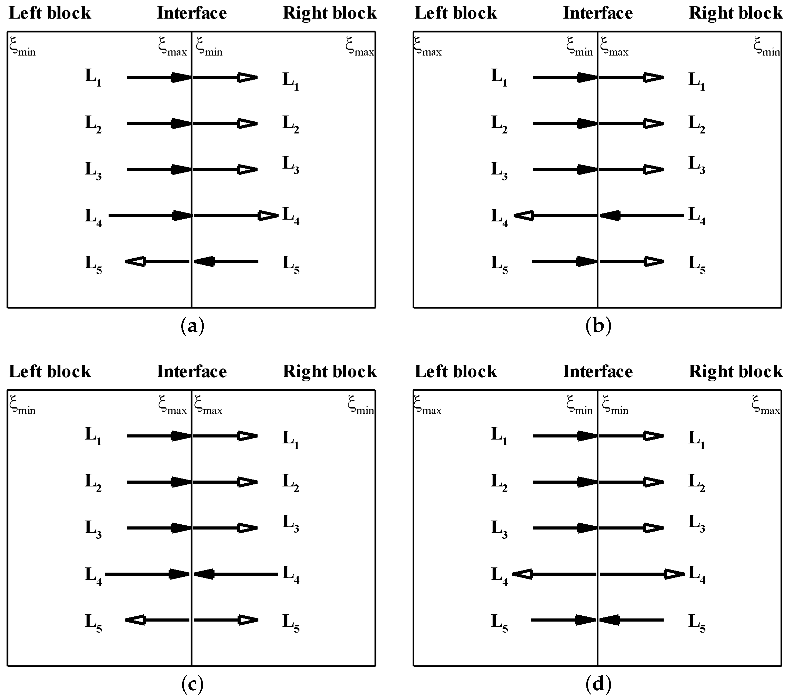
2.7. Interface Matching

In this section, the interface matching process for the flow fields is described. The transfer direction of a characteristic wave component $L_i$ is determined by the eigenvalue of $L_i$, i.e., $\left[U,U,U,U+C,U-C\right]$. Under subsonic conditions, four eigenvalues have a positive sign, and one eigenvalue has a negative sign. Thus, four characteristic waves are travelling from the upstream to the downstream side, and one wave is travelling in the opposite direction. The decision of which wave amplitude needs to be corrected is dependent on whether the convection speed at the interface is larger or smaller than the sound speed. Based on the signs of the contravariant velocities at the block interface, four possible combinations of wave directions can be found, which are shown in Figure 1. The characteristic wave components, denoted by solid arrows, are the known ones, and those with a hollow arrow are unknown ones, which are corrected by the characteristic interface treatment. In all cases, a total of five unknown and five known vectors exist at the interface.

For the supersonic case, all of the eigenvalues are positive. Therefore, all characteristic waves are moving from the left to the right side, i.e., all of the wave amplitudes on the upstream side are self-determined. Hence, the handling of the interface conditions is very different for the two cases. As long as the time integration is achieved accurately from the same initial state, the interface variables of the upstream and the downstream side will be in agreement in arbitrary time. As a result, the interface treatment is considerably simplified and results in the procedure to replace the conservative variables at the downstream side with those at the upstream side.

2.8. Interface Matching of Turbulence Quantities

An efficient matching approach is derived for turbulence quantities in this work. For illustrative purposes, the one-equation turbulence model of Spalart and Allmaras [18] is used. Equation (14) is reorganized as,

$$\frac{\partial }{\partial t}\left(\rho \tilde{\nu }\right)=G_{\nu }-Y_{\nu }+T_s$$

(25)

where

$$T_s=\frac{1}{{\sigma }_{\nu }}\left[\frac{\partial }{\partial x_j}\left\{\left(\mu +\rho \tilde{\nu }\right)\frac{\partial \tilde{\nu }}{\partial x_j}\right\}+C_{b2}\rho {\left(\frac{\partial \tilde{\nu }}{\partial x_j}\right)}^2\right]-\frac{\partial }{\partial x_j}\left(\rho \tilde{\nu }{u}_i\right)$$

(26)

The interface matching of turbulence quantities is based on the simple fact that time developments of the turbulent variables at the upstream limit and those at the downstream limit on the block interface are strictly matched. The production and dissipation terms need also to be the same at the block interface. Based on this simple logic, the matching condition for turbulence quantities can be written as,

$${\left[G_{\nu }-Y_{\nu }+T_s\right]}_{\mathrm{left}}={\left[G_{\nu }-Y_{\nu }+T_s\right]}_{\mathrm{right}}$$

(27)

Equation (27) can be rewritten as,

$${\left[G_{\nu }-Y_{\nu }\right]}_{\mathrm{left}}={\left[G_{\nu }-Y_{\nu }\right]}_{\mathrm{right}}+T_s^r-T_s^l$$

(28)

Using Equation (28), net production and dissipation effects are strictly matched at the interface at each time step. For example, if the computation reaches the left-hand block of Figure 1, then Equation (28) is used to evaluate the net effect of production and dissipation (i.e., the term, $G_{\nu }-Y_{\nu }$) on the left side of the interface by adding the value of ($G_{\nu }-Y_{\nu }$) on the right side of the interface to the difference between the value of $T_s$ on the right and left side of the interface. When the computation reaches the right-hand block, the process is reversed, i.e., the references to left and right in Equation (28) are transposed. As the computation advances iteratively, the process ensures that the time derivative of the turbulence quantity at the block interface (Equation (25)) is correctly matched. The process is equally applicable to two-equation turbulence models, i.e., both of the differential equations for the specific turbulence model can be re-organised in the form of Equation (25).

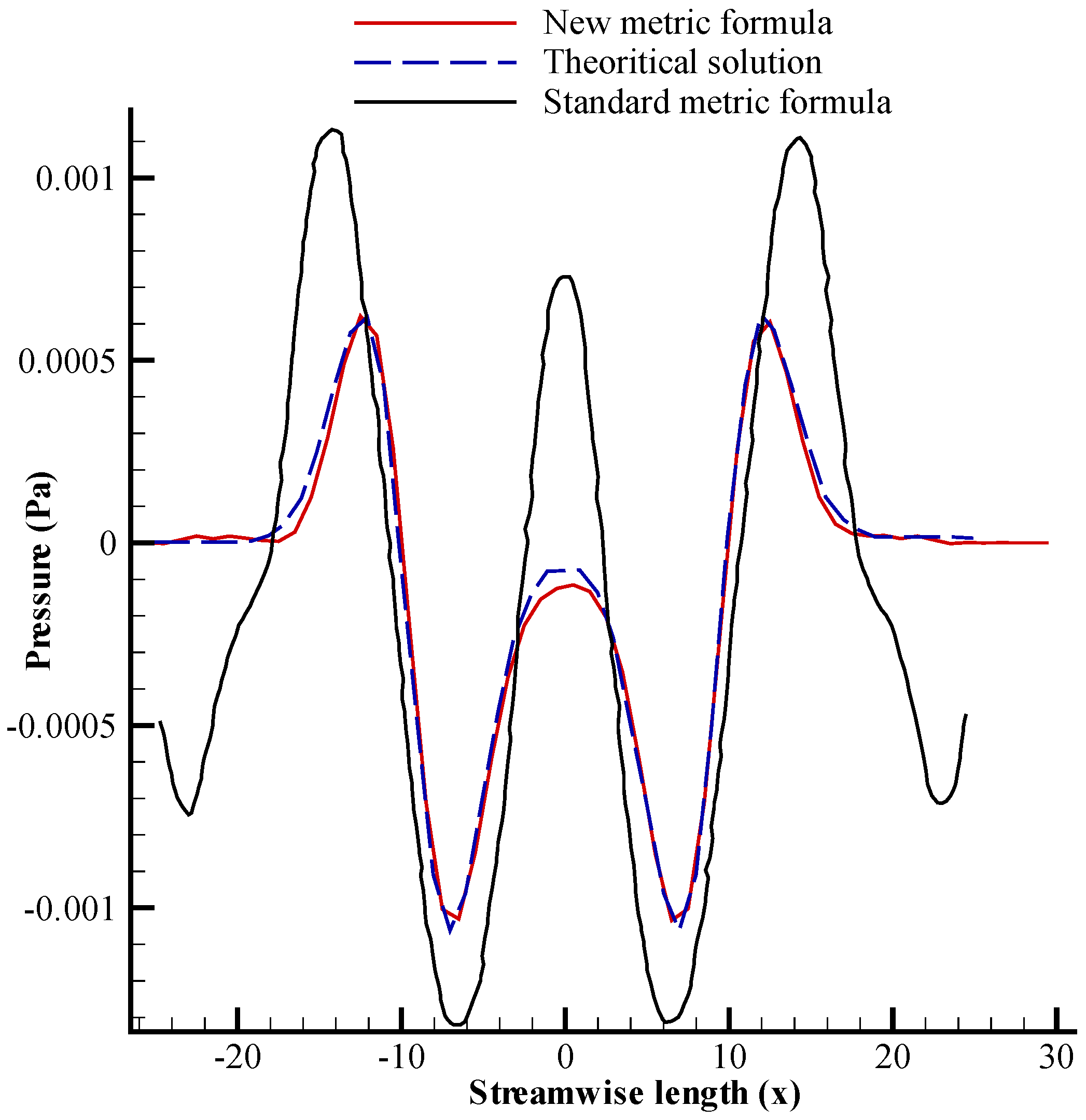
2.9. Metric Cancellation Errors

The fourth-order solver presented here solves the strong-conservation form of the Navier–Stokes equations, which implies that the metric identities in Equations (29) to (31) have been implicitly invoked. Equation (32), which is only applicable to time-variant coordinate systems (i.e., moving meshes), is derived from the grid volume conservation, also widely referred to as the geometric conservation law (GCL) [25,26,27,28]. In any finite-difference discretization scheme, these identities must be satisfied numerically (Equations (29) to (31) for non-moving meshes) in order to ensure free-stream preservation.

$${\left(\frac{{\xi }_x}{J}\right)}_{\xi }+{\left(\frac{{\eta }_x}{J}\right)}_{\eta }+{\left(\frac{{\zeta }_x}{J}\right)}_{\zeta }=0$$

(29)

$${\left(\frac{{\xi }_y}{J}\right)}_{\xi }+{\left(\frac{{\eta }_y}{J}\right)}_{\eta }+{\left(\frac{{\zeta }_y}{J}\right)}_{\zeta }=0$$

(30)

$${\left(\frac{{\xi }_z}{J}\right)}_{\xi }+{\left(\frac{{\eta }_z}{J}\right)}_{\eta }+{\left(\frac{{\zeta }_z}{J}\right)}_{\zeta }=0$$

(31)

$${\left(\frac{1}{J}\right)}_{\tau }+{\left(\frac{{\xi }_t}{J}\right)}_{\xi }+{\left(\frac{{\eta }_t}{J}\right)}_{\eta }+{\left(\frac{{\zeta }_t}{J}\right)}_{\zeta }=0$$

(32)

The issue of free-stream preservation and metric cancellation errors is, therefore, important and has to be ensured in order to extend high-order schemes to non-trivial 3D generalized curvilinear coordinates. These errors arise in finite difference discretizations of governing equations written in strong conservation form and could easily degrade the accuracy of the high-order calculations. Grid-induced errors may appear, for instance, in regions of large grid variations or near singularities. The straight-forward approach to calculating the metrics given in Equation (9) fails to provide metric cancellation for general 3D curvilinear meshes. Evaluation of the y and z derivatives (which are required to calculate ${\xi }_x$, ${\eta }_x$ and ${\zeta }_x$) using compact centred schemes in Equation (9) does not satisfy the metric identity in Equation (29), and therefore, grid-induced errors appear in regions of large grid variation or near singularities. For curvilinear 2D meshes, Pulliam and Steger [25] demonstrated that the compact scheme provided metric cancellation when the metrics were evaluated with the same finite difference scheme as those employed for the computation of fluxes, and they introduced a simple averaging procedure to guarantee the free-stream preservation on 3D curvilinear grids. Although this procedure worked well for a second-order scheme, it is not suitable for high-order solvers. An alternative method to enforce the metric identities can be achieved by using the method of Thomas and Lombard [26], which consists of writing the metric relations in conservative form as:

$$\begin{array}{cc}{\xi }_x=J\left\{\frac{\partial }{\partial \zeta }\left(z\frac{\partial y}{\partial \eta }\right)-\frac{\partial }{\partial \eta }\left(z\frac{\partial y}{\partial \zeta }\right)\right\},& {\xi }_y=J\left\{\frac{\partial }{\partial \zeta }\left(x\frac{\partial z}{\partial \eta }\right)-\frac{\partial }{\partial \eta }\left(x\frac{\partial z}{\partial \zeta }\right)\right\}\\ {\xi }_z=J\left\{\frac{\partial }{\partial \zeta }\left(y\frac{\partial x}{\partial \eta }\right)-\frac{\partial }{\partial \eta }\left(y\frac{\partial x}{\partial \zeta }\right)\right\},& {\eta }_x=J\left\{\frac{\partial }{\partial \xi }\left(z\frac{\partial y}{\partial \zeta }\right)-\frac{\partial }{\partial \zeta }\left(z\frac{\partial y}{\partial \xi }\right)\right\}\\ {\eta }_y=J\left\{\frac{\partial }{\partial \xi }\left(x\frac{\partial z}{\partial \zeta }\right)-\frac{\partial }{\partial \zeta }\left(x\frac{\partial z}{\partial \xi }\right)\right\},& {\eta }_z=J\left\{\frac{\partial }{\partial \xi }\left(y\frac{\partial z}{\partial \zeta }\right)-\frac{\partial }{\partial \xi }\left(y\frac{\partial z}{\partial \zeta }\right)\right\}\\ {\zeta }_x=J\left\{\frac{\partial }{\partial \xi }\left(z\frac{\partial y}{\partial \eta }\right)-\frac{\partial }{\partial \xi }\left(z\frac{\partial y}{\partial \eta }\right)\right\},& {\zeta }_y=J\left\{\frac{\partial }{\partial \eta }\left(x\frac{\partial z}{\partial \xi }\right)-\frac{\partial }{\partial \xi }\left(x\frac{\partial z}{\partial \eta }\right)\right\}\\ & {\zeta }_y=J\left\{\frac{\partial }{\partial \eta }\left(y\frac{\partial x}{\partial \xi }\right)-\frac{\partial }{\partial \xi }\left(y\frac{\partial x}{\partial \eta }\right)\right\}\end{array}$$

(33)

The conservative differential form of Equation (33) is ideally suited to the strong-conservation form of the flow equations solved in the fourth-order solver presented here and is therefore selected for the 3D complex-geometry simulations.

3. Validation

Several test cases, including both inviscid and viscous simulations, were performed to test the performance of the characteristic interface conditions proposed. To illustrate the accuracy of the turbulence matching technique for multi-block grids, fully-turbulent flow past a backward-facing step was also solved. One of the test cases was from the typical CAA benchmark problems used in the validation of CAA codes. All of the computed test cases in this paper are based on 2D geometries. However, the methodology has also been successfully used to simulate 3D flow problems, an example of which can be found in Khanal et al. [29]. All boundary conditions are non-reflecting characteristic domain boundaries. The freestream uses a non-reflecting outflow boundary.

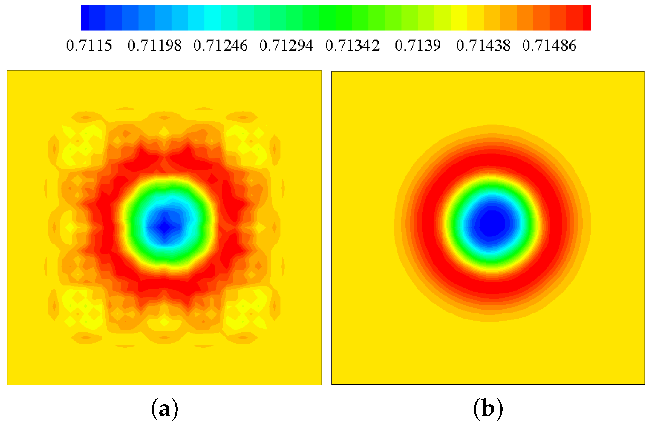
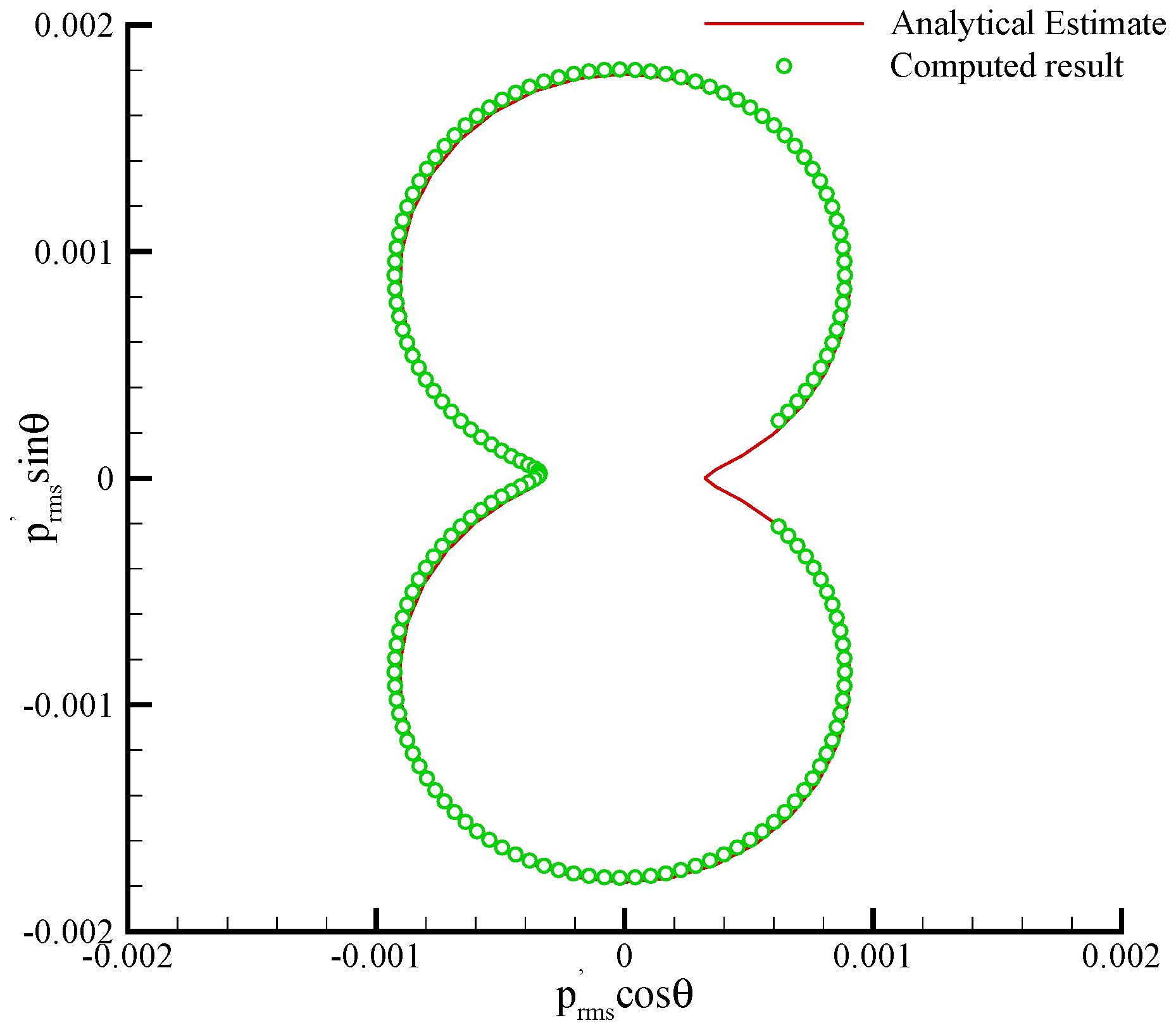
3.1. Two-Dimensional Acoustic Scattering

To demonstrate the accuracy of the CAA solver in multi-dimensions and illustrate the stability and low dispersive behaviour of the solver, a two-dimensional acoustic scattering problem from the Second CAA workshop [30] is considered. The physical problem is to study the scattering of the sound source (generated by a propeller) from the fuselage of an aircraft. The fuselage is idealized as a circular cylinder and the noise source (propeller) as a line source so that the computational domain is 2D. The geometry therefore is a 2D cylinder of non-dimensional radius $R=0.5$ placed at the origin of a cylindrical coordinate system. An acoustic pulse with initial conditions is scattered by the cylinder. The initial conditions for this sound scattering problem are given by,

$$\begin{array}{cc}\hfill p\left(x,y,0\right)& =exp\left[-ln2\left(\frac{{\left(x-4\right)}^2+y^2}{0.04}\right)\right]\hfill \\ \hfill u\left(x,y,0\right)& =0\hfill \\ \hfill v\left(x,y,0\right)& =0\hfill \end{array}$$

(34)

This benchmark problem has been solved previously on an orthogonal grid generated with an O-topology [9]. In the present work, to challenge the stability of the solver, it was solved on a non-orthogonal grid domain generated using the H-topology. The computational domain consists of a square box of $30d$ edge dimension with the cylinder at its centre. The cell distributions near the cylinder surface are shown in Figure 2. The number of grid points is $355\times 220$. Details of the boundary conditions are given by Kim and Lee [10]. An instantaneous plot of the computed pressure field at non-dimensional time $t=5$ is shown in Figure 3 where it can be seen that the acoustic pulse has just reflected off the cylinder. The unsteady pressure history is recorded at three points: A ($r=5;\theta ={90}^{\circ }$), B ($r=5;\theta ={135}^{\circ }$) and C ($r=5;\theta ={180}^{\circ }$) during simulation; $\theta$ is measured from the downstream cylinder axis and is positive counter-clockwise. Figure 4a–c shows these computed pressure time histories in comparison with the analytical solution [30]. The monitor points were placed at three different locations to verify that a highly accurate solution is achieved irrespective of the directional position in the domain. Excellent agreement with the analytical data is evident at all three locations.

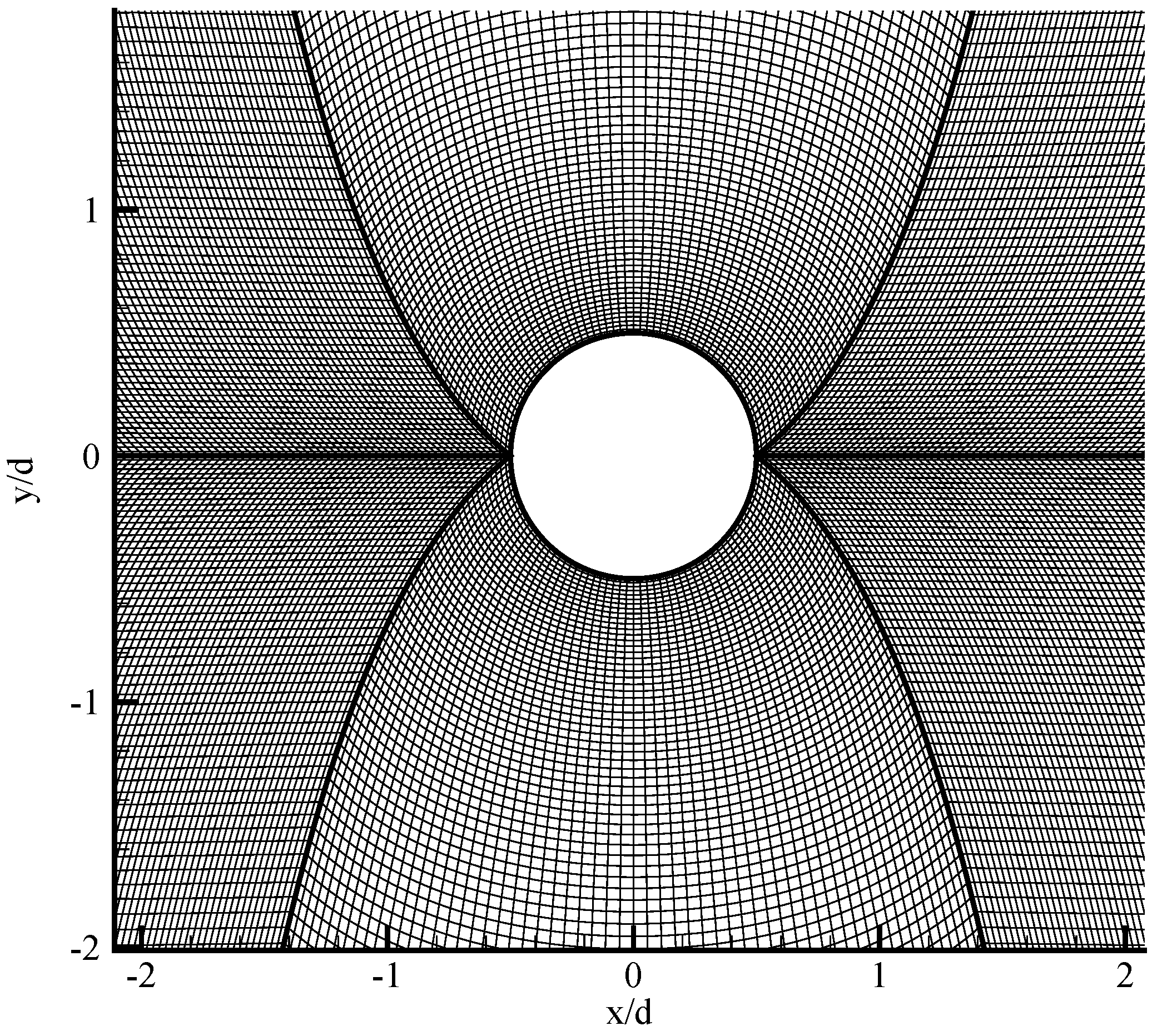
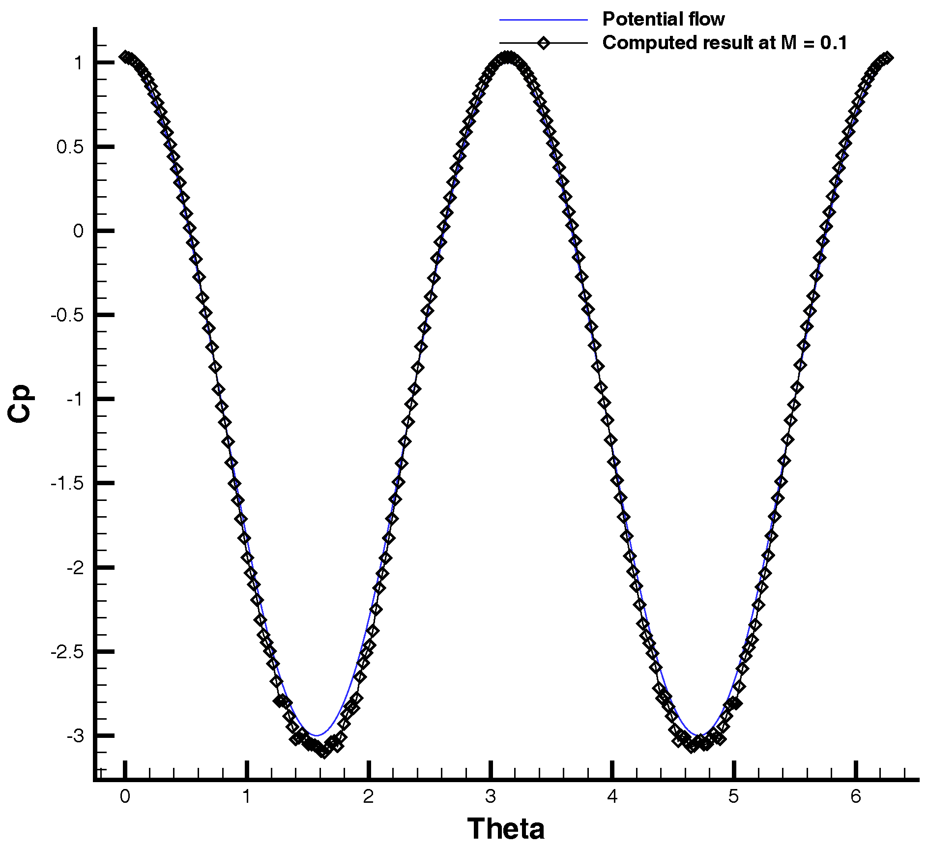
3.2. Inviscid Flow Past a 2D Cylinder

An inviscid flow past a circular cylinder is a steady flow without separation and is close to potential flow in the low-Mach-number regime. The grid domain used was the same H-topology as the one used in the acoustic scattering case. This problem has been solved previously, and the boundary and flow conditions are as described by Kim and Lee [10]. The pressure coefficient curve is plotted in Figure 5 along the cylinder surface in comparison with the potential flow case ($C_p=1-4{sin}^2\theta$). From Figure 5, it is evident that the computed inviscid solution is in good agreement with the analytical potential flow solution.

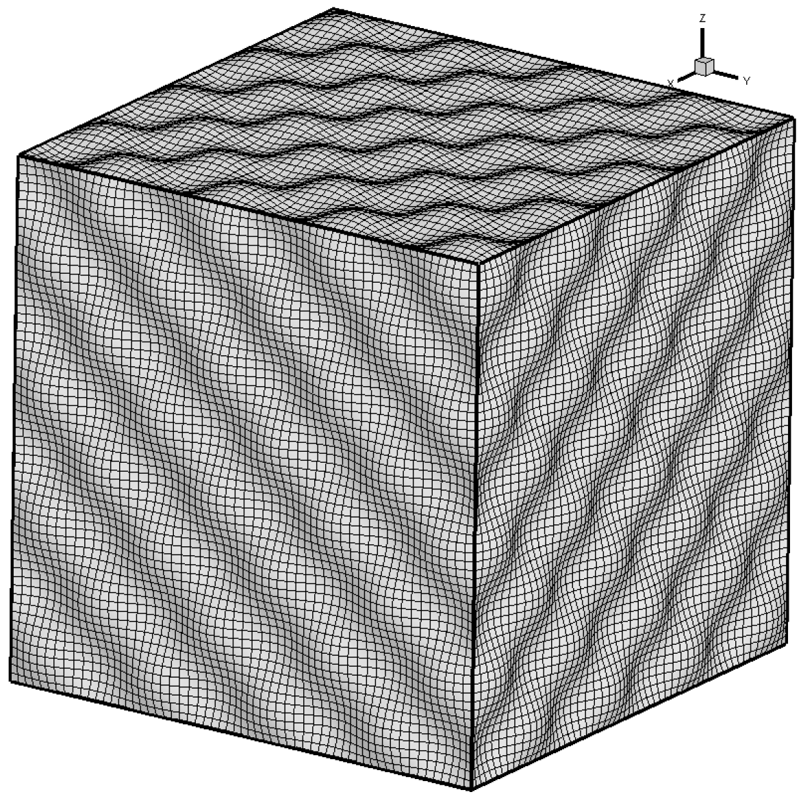
3.3. Sound Propagation in 3D Curvilinear Meshes

For the next validation case, propagation of a 3D spherical acoustic pulse in a curvilinear mesh was computed to evaluate the effect of metric cancellation errors on acoustic propagation. A three-dimensional curvilinear grid was generated using the following equations [28]:

$$\begin{array}{cc}\hfill x(i,j,k)& =x_{\mathrm{ref}}+\delta x\left[(i-1)+sin\left\{\frac{8\pi \left(j-1\right)\delta y}{L_y}\right\}sin\left\{\frac{8\pi \left(k-1\right)\delta z}{L_z}\right\}\right]\hfill \\ \hfill y(i,j,k)& =y_{\mathrm{ref}}+\delta y\left[(j-1)+sin\left\{\frac{8\pi \left(i-1\right)\delta x}{L_x}\right\}sin\left\{\frac{8\pi \left(k-1\right)\delta z}{L_z}\right\}\right]\hfill \\ \hfill z(i,j,k)& =z_{\mathrm{ref}}+\delta z\left[(k-1)+sin\left\{\frac{8\pi \left(i-1\right)\delta x}{L_x}\right\}sin\left\{\frac{8\pi \left(j-1\right)\delta y}{L_y}\right\}\right]\hfill \end{array}$$

(35)

with:

$$\delta x=\frac{L_x}{n_x-1};\delta y=\frac{L_y}{n_y-1};\delta z=\frac{L_z}{n_z-1}$$

and:

$$i=1\dots n_x;j=1\dots n_y;k=1\dots n_z.$$

The domain generated using Equation (35) results in a computational grid that does not satisfy the metric identities discussed earlier, i.e., Equations (29) to (31). An isometric view of the resulting wavy mesh is shown in Figure 6. A 3D spherical acoustic pulse, described by Equation (36), was initiated at the centre of the mesh to study its propagation accuracy in the distorted wavy mesh. All of the outer faces of the grid block were modelled by a characteristic outflow boundary condition.

$$\begin{array}{c}p=p_{\infty }+\epsilon e^{-ln2\left(\frac{x^2+y^2+z^2}{9}\right)}\hfill \\ u\left(x,y,z,0\right)=0\hfill \\ v\left(x,y,z,0\right)=0\hfill \\ w\left(x,y,z,0\right)=0\hfill \end{array}$$

(36)

where $\epsilon =0.01$.

Figure 7a,b displays the calculated pressure contours on a plane through the centre of the spherical pulse at $t=10$ for the case when the metrics are evaluated using Equations (9) and (33), respectively. It is apparent that significant distortion of the acoustic wave occurs due to the lack of freestream preservation, i.e., metric cancellation errors. The acoustic pressure along the grid line $i=j=31$ is compared in Figure 8 with the theoretical solution for both the calculations where the poor performance of the standard metric evaluation method is apparent. The results obtained with the metric evaluation procedure of Equation (33) exhibit no acoustic distortions, and the computed line pressure is in very good agreement with the theory. Hence, even for relatively good quality curvilinear grids, errors resulting from the lack of freestream preservation can corrupt the acoustic pressure significantly unless proper metric evaluation procedures are employed.

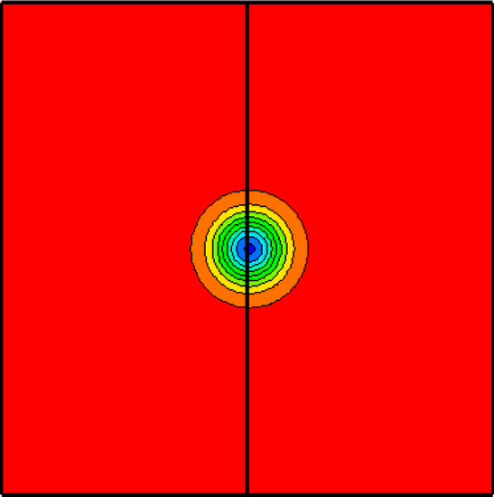
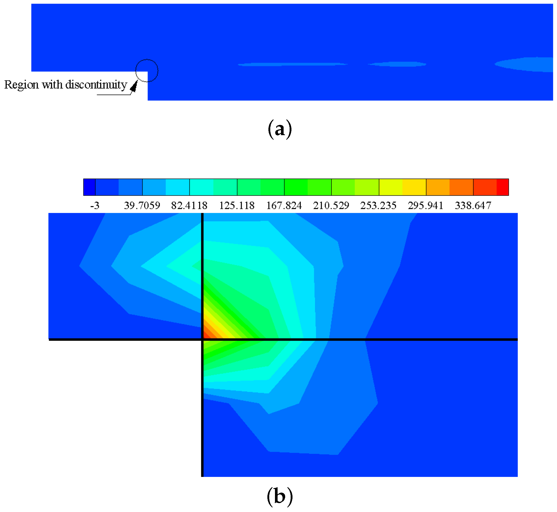
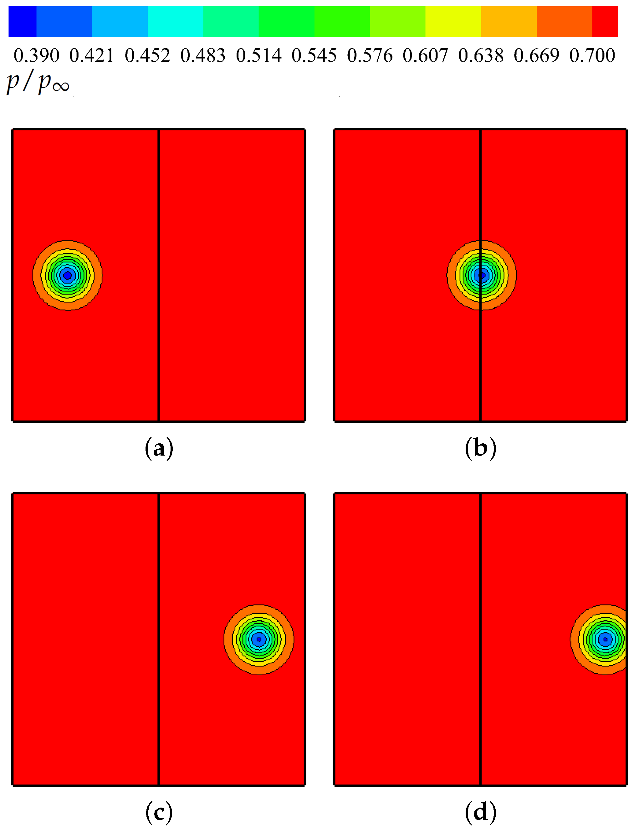
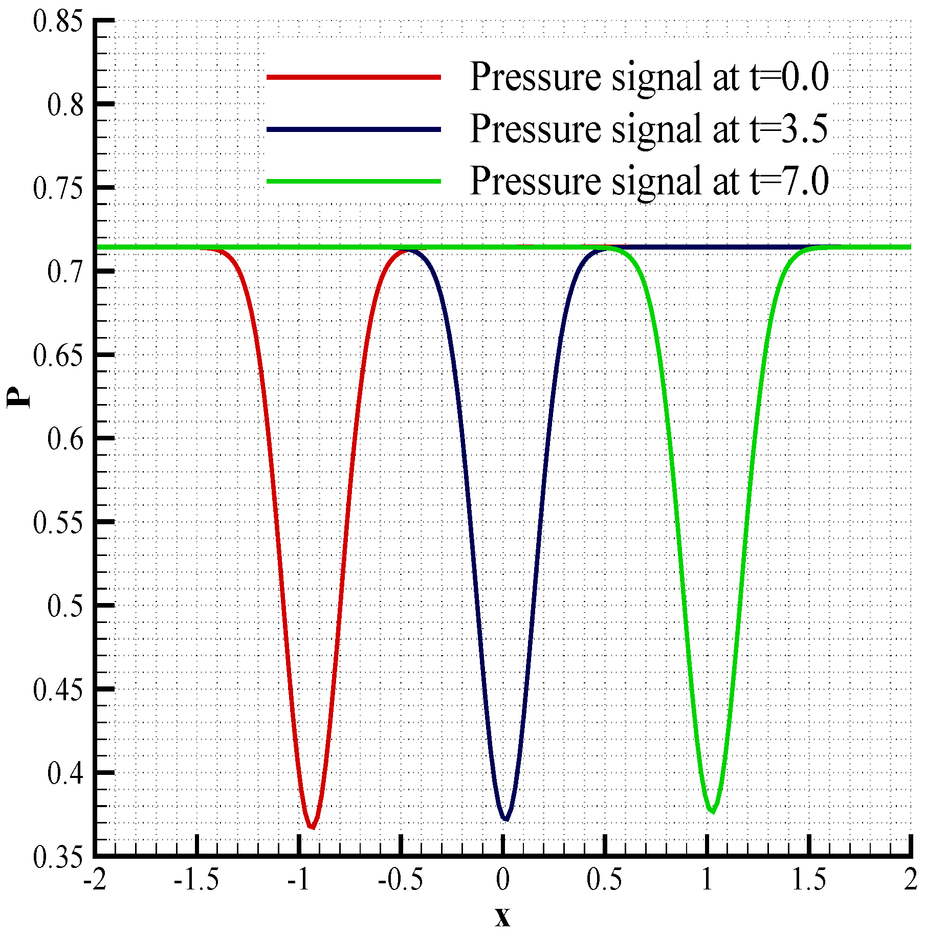
3.4. Vortex Propagation across a Block Interface

To validate the accuracy of the interface matching conditions and demonstrate their transparent behaviour towards acoustic waves, a two-dimensional problem of an isentropic vortex convection across a block interface is considered. The Mach number of this case is taken to be $0.3$, and the Reynolds number in viscous flow is set to be ${10}^4$. A single convective vortex in an uniform flow is expressed as,

$$\begin{array}{cc}\hfill p& =p_{\infty }-\frac{\rho C_0^2}{2R_0^2}exp(-r^2)\hfill \\ \hfill u& =u_{\infty }-\frac{C_0\left(y-y_c\right)}{R_0^2}exp(-r^2/2)\hfill \\ \hfill v& =\frac{C_0\left(x-x_c\right)}{R_0^2}exp(-r^2/2)\hfill \end{array}$$

(37)

where:

$$r^2=\frac{{\left(x-x_c\right)}^2+{\left(y-y_c\right)}^2}{R_0^2}$$

and $C_0$ and $R_0$ are set to $0.167$ and $0.2$, respectively [14]. Each of the blocks had grid dimensions of $121\times 241$. Further details on the flow and boundary conditions are given by Sumi and Kurotaki [14]. The vortex is initially released from $(x_c,y_c)=-(1,0)$ at $t=0$. The pressure contours of the propagating vortex at four different instances is shown in Figure 9. It can be seen that the vortex passes through the block interface boundary very smoothly, and there is no evidence of acoustic reflections or any other instabilities. The pressure signal along a horizontal line through the centre of the convecting vortex corresponding to the first three instances in Figure 9 is plotted in Figure 10. As can be seen there is no reflection of the signals at the block interface, and it is found to pass smoothly. The interface condition is transparent, therefore, to the vortex propagation problem.

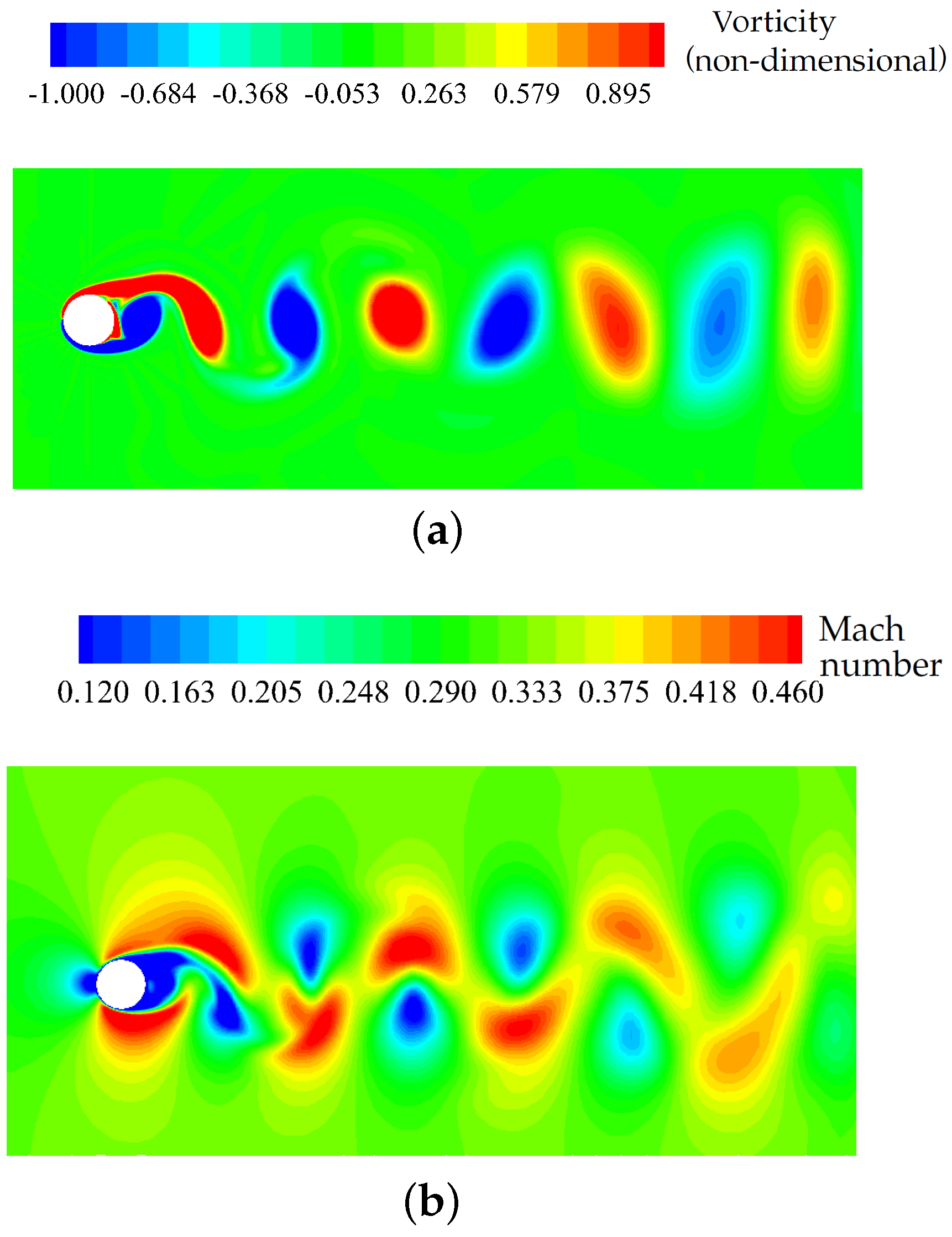
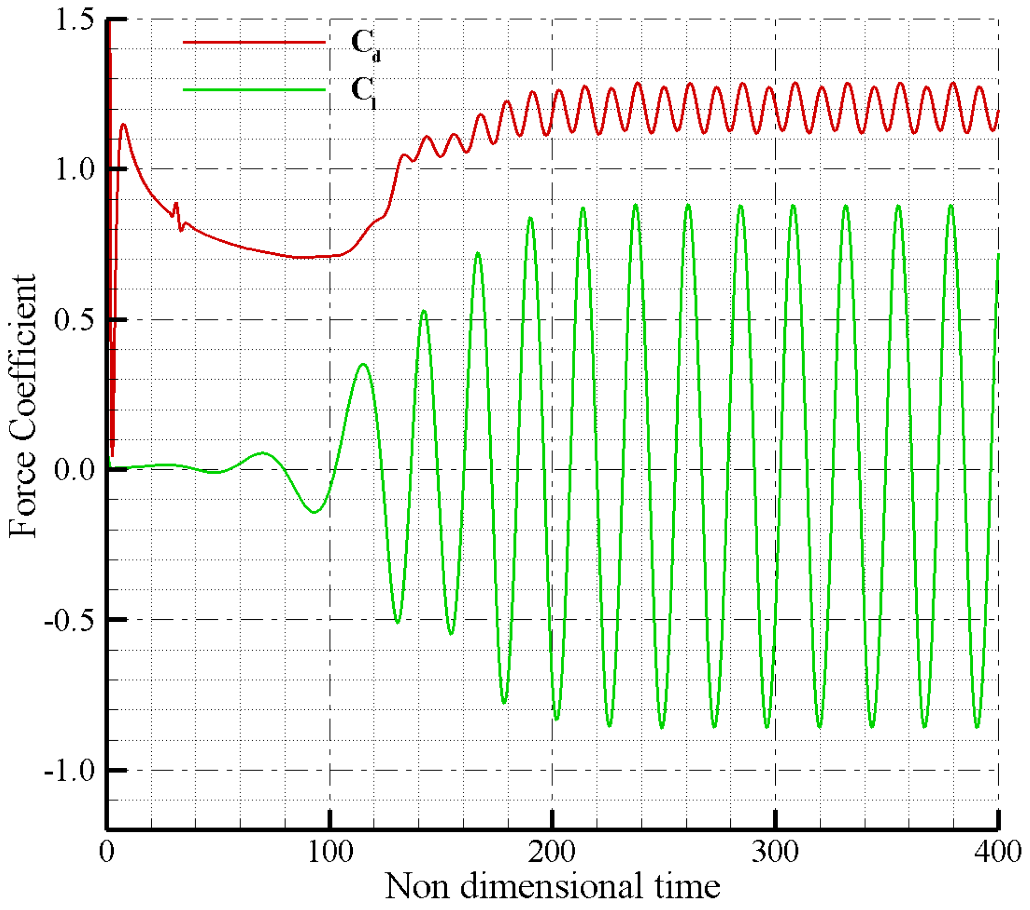
3.5. Laminar Flow Past a 2D Cylinder

Viscous flow past a circular cylinder is found to shed vortices in the well-known von Kármán vortex street behind the cylinder. It is known experimentally that a regular von Kármán street exists when the flow Reynolds number (based on cylinder diameter) lies in the range of about 60 to 5000 [31], and the Strouhal number depends only on Reynolds number in this range. This regular vortex shedding causes fluctuations in lift and drag forces, which results in the radiation of a dipole sound field. The radiated dipole sound is estimated analytically and compared with the computational result. The analytical formula neglects the effects of quadrupole sources due to the convection of vortices; however, the quadrupole source strength is negligibly small at low subsonic speeds compared to the dipole source. The analytical formula, therefore, is well suited for predicting sound directivity for low subsonic flows and is used in this work for comparison with the computed result. The analytical formula used to predict the dipole sound directivity can be written as [10],

$$p_{\mathrm{rms}}^{\prime }\left(r,\theta \right)=\frac{{\rho }_{\infty }{a}_{\infty }^2}{4}{\left[\right\{\frac{M_{\infty }^5\mathrm{St}}{\raisebox{1ex}{$r$}\!\left/ \!\raisebox{-1ex}{$d$}\right.}\left\}\left\{\overline{C_L^2}{sin}^2\theta +4\overline{{\left(C_D-\overline{C_D}\right)}^2}{cos}^2\theta \right\}\right]}^{\frac{1}{2}}$$

(38)

where St is the Strouhal Number, r is the distance from the centre of the cylinder and d is the cylinder diameter.

As with the inviscid case, a non-orthogonal grid generated using an H-topology was used for the viscous flow simulation about a 2D cylinder. The flow Reynolds number, based on the cylinder diameter and a Mach number of 0.3, was 300. The number of grid points used was $250\times 150$. The grid points were clustered near the cylinder wall, and the boundary layer was resolved by approximately 25 grid points normal to the cylinder surface. All of the flow and boundary conditions for this case are taken from Kim and Lee [10].

The simulation was run with a Courant–Friedrichs–Lewy (CFL) number of $0.5$ and was continued until the non-dimensional time reached $t\times a_{\infty }/d=400$. Figure 11 shows contours of the instantaneous vorticity and velocity fields at the end of the computation; this clearly indicates the existence of a von Kármán street along with the positions of the vortices. Time-dependent lift and drag coefficients are plotted in Figure 12 showing, after initial transients have settled, a periodic fluctuation of unsteady forces with constant magnitudes at a constant frequency. The frequency of this periodic oscillation was used to evaluate the Strouhal number. The computed values of the Strouhal number, mean drag coefficient and rms fluctuating lift coefficient are compared with experimental data [10,31] and listed in

Table 1. Strouhal Number and mean force coefficients for laminar flow past a 2D cylinder.

Cases	Strouhal Number (St)	Drag Coefficient ($\overline{{\mathit{C}}_{\mathit{d}}}$)	rms Lift Coefficient $(\overline{{\mathit{C}}_{\mathit{l}}^2}{)}^{\frac{1}{2}}$
Experiment	$0.21\pm 0.005$	$1.2\pm 0.1$	$0.6\pm 0.1$
Computed	0.212	1.202	0.612

. From the results, the mean flow properties computed using the proposed boundary conditions are found to agree well with the experiment. Figure 13 compares the computed acoustic directivity with the analytical estimation using Equation (38). The computed result is in very good agreement with the analytical approximation demonstrating the low acoustic dispersion and dissipation characteristics of the solver.

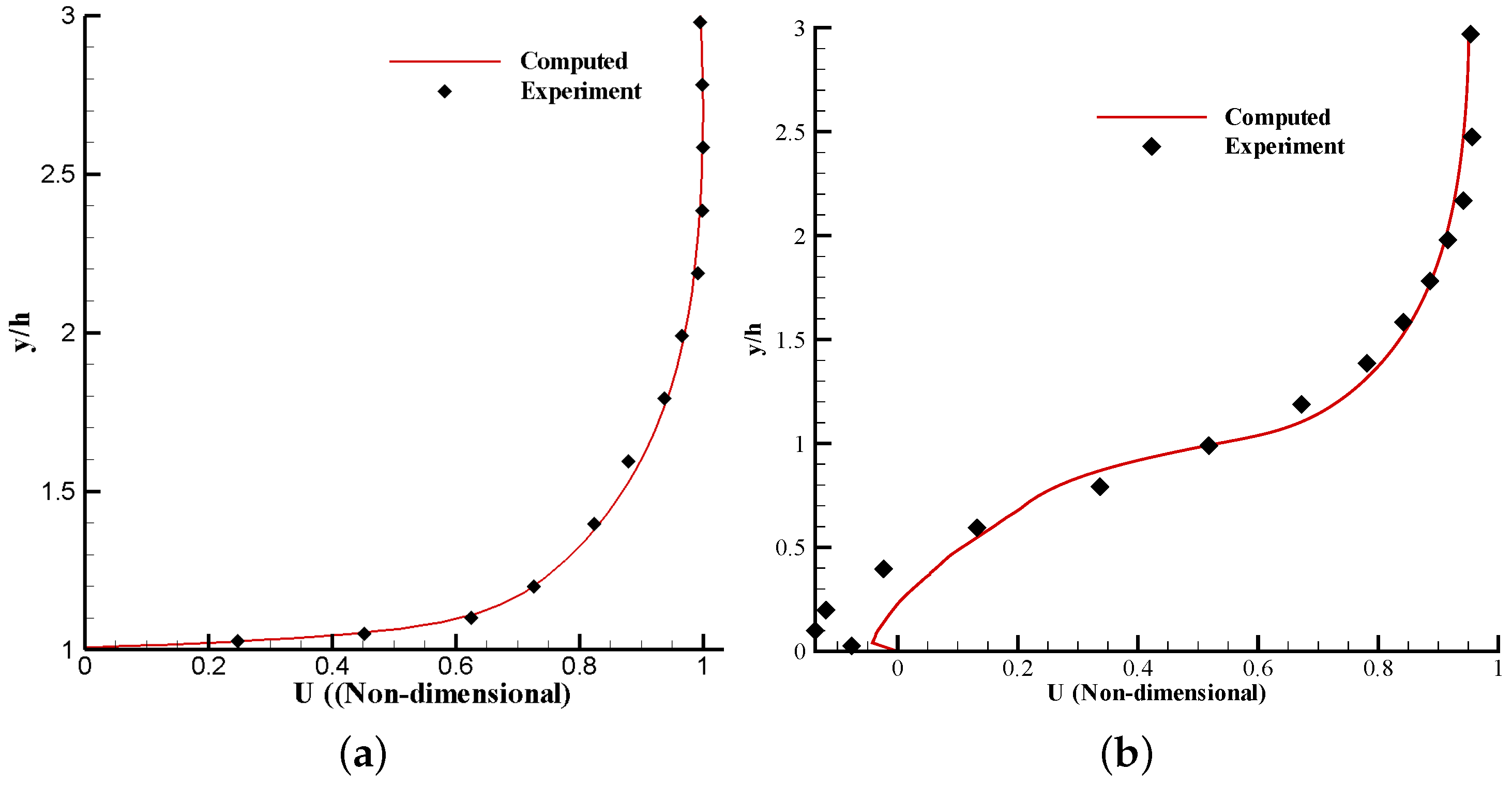
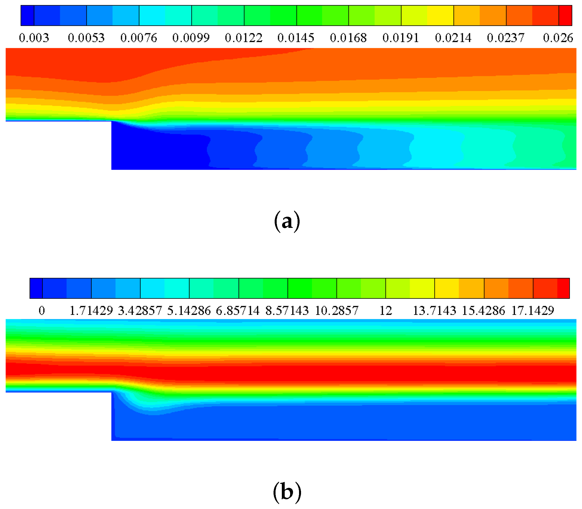
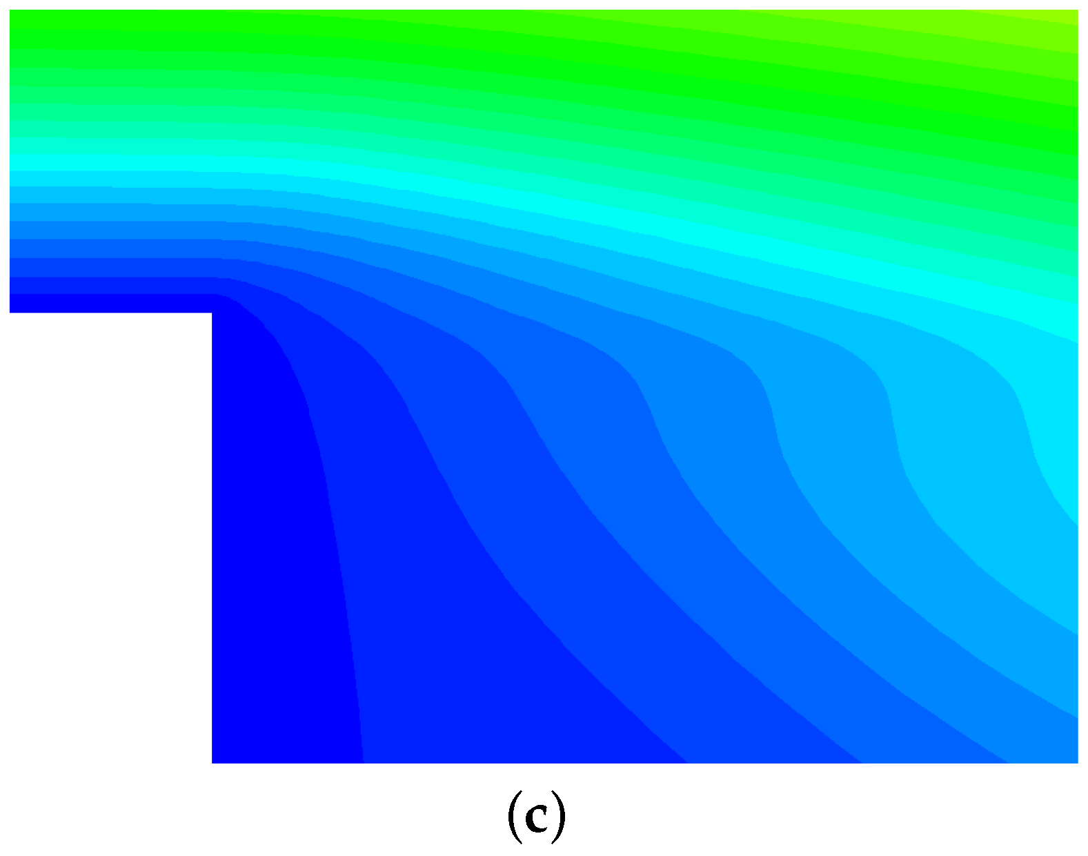
3.6. Turbulent Flow Past a Backward-Facing Step

Having demonstrated the good accuracy of the solver in computing acoustic scattering, potential flow past a cylinder and viscous laminar flow, a viscous turbulent calculation was performed to demonstrate the performance of the turbulence matching. For this case, a backward-facing step was chosen, owing to the ready availability of high-quality experimental data. The computational domain was designed using a structured multi-block strategy. The computational domain consisted of eight structured blocks. Along the inflow boundary, the two Cartesian velocity components $u,v$ together with the turbulence quantity ${\nu }_t$ were prescribed to ensure that the computed boundary layer profile matched the experiment of Jovic and Driver [32]. These values were determined using Wilcox’s EDDYBL boundary layer program [33], together with knowledge of the experimental boundary layer profile upstream of the step. In total, the computational grid consisted of approximately 33,000 cells. To resolve the shear and boundary layers, grid cells are clustered along all solid walls, as well as around the step region using a hyperbolic tangent distribution function. In all cases, the meshes were designed to ensure a $y^{+}$ of less than or equal to one along all solid walls. Upstream of the step, the boundary layer was resolved with a minimum of 25 mesh points. In the experiment [32], the backward-facing step flow was found to be closely represented by a two-dimensional flow in the measurement domain. Hence, in accordance with the experimental observation, a two-dimensional simulation was performed in this case. The step and flat plate were modelled as an adiabatic wall. All of the other boundary faces were modelled to be characteristic outflow. Details on the flow and geometrical conditions for this case are given by Jovic and Driver [32].

Computations were performed using both the new matching procedure and the existing approaches (based on simple averaging) at the block-interfaces. From the result, a discontinuity was found to exist in turbulence variables (${\mu }_t$ and ${\nu }_t$) at block interfaces when the turbulence quantities at the interface were matched using simple averaging. Contours of non-dimensional kinematic turbulent viscosity are plotted in Figure 14 for the result using standard averaging, and a clear discontinuity is found to exist at the three-block-interface junction. This discontinuity, however, is not present in the result from the new interface treatment (Figure 15), and a smooth and continuous solution is found to exist at all of the block interfaces. Comparisons of mean streamwise velocity profiles with experiment at two different locations are plotted in Figure 16. A reasonably good agreement between the experiment and the computed result is evident. Hence, the proposed method to match turbulence quantities at the block interfaces completes the extension of characteristic-based interface matching methods for turbulent flow simulation with improved accuracy and robustness.

4. Conclusions

A computational aeroacoustics solver, which uses a high-order accurate compact finite-difference scheme, has been developed to compute aerodynamic noise-generation problems with high accuracy. The solver is based on a hybrid strategy, which combines near-field numerical simulations with a far-field radiation model. An extensive set of two-dimensional numerical simulations was performed to validate the solver. All of the computed results were found to agree well with experiments, in both frequency and magnitude. The computed results presented have demonstrated the capability of the CAA solver to resolve unsteady flow fields accurately for a wide range of geometries and flow conditions. The solver is found to perform robustly with complex multi-block curvilinear structured grids despite having no artificial dissipation.

References

1. Singer, B.A.; Guo, Y. Development of computational aeroacoustic tools for airframe noise calculations. Int. J. Comput. Fluid D. 2004, 18, 455–469. [Google Scholar] [CrossRef]
2. Tam, C.K.W. Computational acoustics: Issues and methods. AIAA J. 1995, 33, 1788–1796. [Google Scholar] [CrossRef]
3. Tam, C.K.W.; Webb, J.C. Dispersion-Relation-Perserving finite difference schemes for computational acoustics. J. Comput. Phys. 1993, 107, 262–281. [Google Scholar] [CrossRef]
4. Kim, J.W.; Lee, D.J. Optimised compact finite difference schemes with maximum resolution. AIAA J. 1996, 34, 887–893. [Google Scholar] [CrossRef]
5. Hixon, R. Prefactored small-stencil compact schemes. J. Comput. Phys. 2000, 165, 522–541. [Google Scholar] [CrossRef]
6. Thompson, K.W. Time dependent boundary conditions for hyperbolic systems. J. Comput. Phys. 1987, 68, 1–24. [Google Scholar] [CrossRef]
7. Thompson, K.W. Time dependent boundary conditions for hyperbolic systems II. J. Comput. Phys. 1990, 89, 439–461. [Google Scholar] [CrossRef]
8. Lele, S.K. Compact finite difference schemes with spectral-like resolution. J. Comput. Phys. 1992, 103, 16–42. [Google Scholar] [CrossRef]
9. Kim, J.W.; Lee, D.J. Generalized characteristic boundary conditions for computational aeroacoustics. AIAA J. 2000, 38, 2040–2049. [Google Scholar] [CrossRef]
10. Kim, J.W.; Lee, D.J. Generalized characteristic boundary conditions for computational aeroacoustics, Part 2. AIAA J. 2004, 42, 47–55. [Google Scholar] [CrossRef]
11. Sunderland, J.C.; Kennedy, C.A. Improved boundary conditions for viscous, reacting, compressible flows. J. Comput. Phys. 2003, 191, 502–524. [Google Scholar] [CrossRef]
12. Yoo, C.S.; Wang, Y.; Trouve, A.; Im, H.G. Characteristic boundary conditions for direct simulations of turbulent counterflow flames. Combust. Theor. Model. 2005, 9, 617–646. [Google Scholar] [CrossRef]
13. Yoo, C.S.; Im, H.G. Characteristic boundary conditions for simulations of compressible reacting flows with multi-dimensional, viscous and reaction effects. Combust. Theor. Model. 2007, 11, 259–286. [Google Scholar] [CrossRef]
14. Sumi, T.; Kurotaki, T. Generalized characteristic interface conditions for accurate multi-block computations. In Proceedings of the 44th AIAA Aerospace Sciences Meeting and Exhibit, Reno, NV, USA, 9–12 January 2006. Number AIAA-2006-1272. [Google Scholar]
15. Kim, J.W.; Lee, D.J. Characteristic interface conditions for multiblock high-order computation on singular structured grid. AIAA J. 2003, 41, 2341–2348. [Google Scholar] [CrossRef]
16. Sumi, T.; Kurotaki, T.; Hiyama, J. Practical multi-block computations with generalized characteristic interface conditions around complex geometry. In Proceedings of the 18th AIAA Computational Fluid Dynamics Conference, Miami, FL, USA, 25–28 June 2007. Number AIAA-2007-4471. [Google Scholar]
17. Chen, X.; Zha, G.C. Implicit application of non-reflective boundary conditions for Navier-Stokes equations in generalized coordinates. Int. J. Numer. Methods Fluids 2006, 50, 767–793. [Google Scholar] [CrossRef]
18. Spalart, P.R.; Allmaras, S.R. A one-equation turbulence model for aerodynamic flows. In Proceedings of the 30th AIAA Aerospace Sciences Meeting and Exhibit, Reno, NV, USA, 6–9 January 1992. Number AIAA-1992-0439. [Google Scholar]
19. Spalart, P.R.; Allmaras, S.R. Comments on the feasibility of LES for wings and on a hybrid RANS/LES approach. Proceedings of First AFOSR International Conference on DNS/LES, Ruston, LA, USA, 4–8 August 1997. [Google Scholar]
20. Spalart, P.R.; Deck, S.; Shur, M.L.; Squires, K.D.; Strelets, M.K.; Travin, A. A new version of detached-eddy simulation, resistant to ambiguous grid densities. Theor. Comp. Fluid Dyn. 2006, 20, 181–195. [Google Scholar] [CrossRef]
21. Kim, J.W. Optimised boundary compact finite difference schemes for computational aeroacoustics. J. Comput. Phys. 2007, 225, 995–1019. [Google Scholar] [CrossRef]
22. Hu, F.Q.; Hussaini, M.Y.; Manthey, J. Low-dissipation and -dispersion Runge-Kutta schemes for computational acoustics. J. Comput. Phys. 1996, 124, 177–191. [Google Scholar] [CrossRef]
23. Visbal, M.R.; Gaitonde, D.V. On the use of higher-order finite-difference schemes on curvilinear and deforming meshes. J. Comput. Phys. 2002, 181, 155–185. [Google Scholar] [CrossRef]
24. Khanal, B. Numerical Modelling of Cavity Flow and Noise. Ph.D. Thesis, Cranfield University, Shrivenham, Swindon, UK, 2010. [Google Scholar]
25. Pulliam, T.H.; Steger, J.L. Implicit finite difference simulation of three dimensional compressible flows. AIAA J. 1980, 18, 159–167. [Google Scholar] [CrossRef]
26. Thomas, P.D.; Lombard, C.K. Geometric conservation law and its application to flow computations on moving grids. AIAA J. 1979, 17, 1030–1058. [Google Scholar] [CrossRef]
27. Chung, Y.M.; Tucker, P.G. Accuracy of higher-order finite difference schemes on non-uniform grids. AIAA J. 2003, 41, 1609–1611. [Google Scholar] [CrossRef]
28. Visbal, M.R.; Gaitonde, D.V. Very high-order spatially implicit schemes for computational acoustics on curvilinear meshes. J. Comput. Acoust. 2001, 9, 1259–1286. [Google Scholar] [CrossRef]
29. Khanal, B.; Knowles, K.; Saddington, A.J. Study of cavity unsteady flowfield. In Proceedings of the 4th International Symposium on Integrating CFD and Experiments in Aerodynamics, Sint-Genesius-Rode, Belgium, 14–16 September 2009. [Google Scholar]
30. Tam, C.K.W.; Hardin, J.C. Second Computational Aeroacoustics Workshop on Benchmark Problems; Technical Report CP-1997-3352; NASA Langley Research Center: Hampton, VA, USA, 1997.
31. Schlichting, H. Boundary-Layer Theory, 7th ed.; McGraw Hill: New York, NY, USA, 1979. [Google Scholar]
32. Jovic, S.; Driver, D.M. Backward-Facing Step Measurements at Low Reynolds Number, Reh = 5000; Technical Report TM-1994-108807; NASA Ames Research Center: Mountain View, CA, USA, 1994.
33. Wilcox, D.C. Turbulence Modelling for CFD, 3rd ed.; DCW Industries: La Cañada Flintridge, CA, USA, 2006. [Google Scholar]
34. Forsyth, A.R. A Treatise on Differential Equations, 3rd ed.; Macmillan and Co. Ltd.: London, UK, 1903. [Google Scholar]
Figure 1. Various block grid orientations and the direction of characteristic waves at the interface. (a) 0 < U l < C , 0 < U r < C ; (b) C < U l < 0 , C < U r < 0 ; (c) 0 < U l < C , C < U r < 0 ; (d) C < U l < 0 , 0 < U r < C .
Aerospace 04 00029 g001
Figure 2. H-topology domain and grid distribution for 2D acoustic scattering; grid points near the cylinder surface (every other point shown).
Aerospace 04 00029 g002
Figure 3. Pressure contours showing acoustic scattering off a 2D cylinder; monitor points A, B and C are described in the text and their pressure-time histories are plotted in Figure 4.
Aerospace 04 00029 g003
Figure 4. Comparison between computed and analytical pressure signals for acoustic scattering off a 2D cylinder ( numerical, — analytical). (a) Time history of monitor Point A shown in Figure 3; (b) Time history of monitor Point B shown in Figure 3; (c) Time history of monitor Point C shown in Figure 3.
Aerospace 04 00029 g004aAerospace 04 00029 g004b
Figure 5. Comparison between potential flow and computational pressure coefficients for acoustic scattering off of a cylinder.
Aerospace 04 00029 g005
Figure 6. Wavy grid to test the metric cancellation errors in 3D sound propagation.
Aerospace 04 00029 g006
Figure 7. Instantaneous acoustic pressure at the central plane (2D xy plane) of a 3D sound propagation showing the superior performance of the new metric evaluation procedure. (a) Standard metric formula; (b) New metric formula.
Aerospace 04 00029 g007
Figure 8. Comparison of computed pressure with the analytical solution showing the superior performance of the new metric cancellation method.
Aerospace 04 00029 g008
Figure 9. Pressure contours showing vortex convection across a block-interface boundary and illustrating its transparent nature to the flow. (a) t × a / L r e f = 0 ; (b) t × a / L r e f = 3.5 ; (c) t × a / L r e f = 7 ; (d) t × a / L r e f = 7.8 .
Aerospace 04 00029 g009
Figure 10. Computed pressure signals at three different times (corresponding to Figure 9a–c) for a convected vortex.
Aerospace 04 00029 g010
Figure 11. Snapshot of instantaneous flow field at t × a / d = 400 for laminar flow past a 2D cylinder. (a) Contours of vorticity magnitude; (b) Contours of velocity magnitude.
Aerospace 04 00029 g011
Figure 12. Fluctuating force coefficients for laminar flow past a 2D cylinder.
Aerospace 04 00029 g012
Figure 13. Comparison of computed analytical acoustic directivity for flow past a 2D cylinder.
Aerospace 04 00029 g013
Figure 14. Contours of normalised mean turbulent kinematic viscosity ( ν t / ν ) for a 2D backward-facing step using a standard block interface treatment and illustrating the unnatural discontinuity introduced by the three-block interface. Note that ν is the freestream reference value of kinematic viscosity ( 1.46 × 10 5 ). (a) Full domain view; (b) Detail at the block interface (zoomed-in view).
Aerospace 04 00029 g014
Figure 15. Mean flow contours for a 2D backward-facing step using the new block interface treatment. Note that the normalised turbulent viscosity ( ν t / ν ) varies smoothly across the block-interfaces, which are transparent to the flow. (a) Contours of mean velocity magnitude ( U / U ); (b) Contours mean normalised turbulent kinematic viscosity ( ν t / ν ); (c) Zoomed-in view of Figure 15b at the block interface.
Aerospace 04 00029 g015aAerospace 04 00029 g015b
Figure 16. Mean velocity profiles for a 2D backward facing step. (a) Velocity profile at x / h = 3.12 ; (b) Velocity profile at x / h = 4 .
Aerospace 04 00029 g016