Assessing the Ability of the DDES Turbulence Modeling Approach to Simulate the Wake of a Bluff Body


1
CFD Laboratory LMFN, Département de Génie Mécanique, Université Laval, 1065 Avenue de la Médecine, Québec, QC G1V 0A6, Canada
2
Graduate Aerospace Laboratories, California Institute of Technology, Pasadena, CA 91125, USA
*
Author to whom correspondence should be addressed.
Aerospace 2017, 4(3), 41; https://doi.org/10.3390/aerospace4030041
Submission received: 26 June 2017
/
Revised: 26 July 2017
/
Accepted: 28 July 2017
/
Published: 1 August 2017
(This article belongs to the Special Issue Computational Aerodynamic Modeling of Aerospace Vehicles)
Abstract
:A detailed numerical investigation of the flow behind a square cylinder at a Reynolds number of 21,400 is conducted to assess the ability of the delayed detached-eddy simulation (DDES) modeling approach to accurately predict the velocity recovery in the wake of a bluff body. Three-dimensional unsteady Reynolds-averaged Navier–Stokes (URANS) and DDES simulations making use of the Spalart–Allmaras turbulence model are carried out using the open-source computational fluid dynamics (CFD) toolbox OpenFOAM-2.1.x, and are compared with available experimental velocity measurements. It is found that the DDES simulation tends to overestimate the averaged streamwise velocity component, especially in the near wake, but a better agreement with the experimental data is observed further downstream of the body. The velocity fluctuations also match reasonably well with the experimental data. Moreover, it is found that the spanwise domain length has a significant impact on the flow, especially regarding the fluctuations of the drag coefficient. Nonetheless, for both the averaged and fluctuating velocity components, the DDES approach is shown to be superior to the URANS approach. Therefore, for engineering purposes, it is found that the DDES approach is a suitable choice to simulate and characterize the velocity recovery in a wake.
1. Introduction
Numerical simulations of turbulent flows involving multiple interacting bodies are of great interest in a large variety of disciplines. Studies on wind farms, the flow around buildings in a city, heat exchangers, or vehicles in close proximity, come to mind. For such studies, an accurate modeling of the wakes is crucial but challenging. It should be noted that one is often not only interested in the mean quantities of the flow in order to characterize a wake, but also in obtaining accurate information regarding the unsteadiness and the turbulence of the flow field. As a result, steady Reynolds-averaged Navier–Stokes (RANS) models are inadequate for the task as they solely provide the averaged quantities. Moreover, even the averaged quantities in a wake predicted with steady RANS modeling can prove to be unreliable [1,2,3]. Further, the unsteady RANS alternative (URANS) often predicts a flow field which is almost periodic in time without significant amplitude modulations in the temporal signals of the physical quantities [2,4]. This often turns out not to be representative of the reality, especially when separation occurs [5]. The large eddy simulation (LES) approach would resolve these issues, but its computation cost makes it impractical for simulating complete turbines operating at high Reynolds number under various operating conditions. One possible solution is the use of a hybrid approach such as the delayed detached-eddy simulations (DDES) technique [3,6], which uses a RANS approach in the attached boundary layers and a LES approach in the separated regions of the flow.
Initially, the detached-eddy simulation methodology has been developed to obtain accurate force predictions on bodies with massively separated flow. A list of successful examples of the application of the detached-eddy simulation (DES) approach for several different geometries is given in the review paper of Spalart [3]. More recently, some researchers have started to show some interest in this turbulence modeling approach for the simulation of turbulent wakes. Among such studies, Paik et al. [7] compared the performances of the URANS approach to different DES methodologies for the flow around two wall-mounted cubes in tandem, Nasif et al. [8] investigated the wake characteristics of sharp-edged bluff body in a shallow flow, Muld et al. [9] observed the flow structures in the wake of a high-speed train and Muscari et al. [1] used this approach to study the wake of a marine propeller and observed a good agreement with the experimental results of Felli et al. [10]. Lastly, the authors of the current work have also used this turbulence modeling approach to study the vortex dynamics and the wake recovery of two different types of hydrokinetic turbines, namely the horizontal axis and the vertical axis turbines [11].
While the capacity of the DDES approach for providing accurate force predictions for bodies with massively separated flows has been largely investigated in the literature, its performances in modeling turbulent wakes have attracted much less attention. In this context, a benchmark case is revisited with the current state-of-the-art numerical methodology making the use of the innovative DDES approach. As the ability of the RANS technique to model attached boundary layers has already been addressed and is well documented [12], this study mainly focus on the performances of the DDES approach in the separated regions of the flow. The sharp-edged square-cylinder case studied experimentally by Lyn et al. [13] at a Reynolds number of 21,400 has been chosen here to achieve this task because its wake dynamics are not dependent on the RANS modeling inherent to a DDES simulation. This is due to the fact that the boundary layers on the upstream face of the square cylinder are laminar and because the separation occurs at fixed locations, namely the upstream sharp edges.
Although the case of Lyn et al. [13] has already been investigated during two LES workshops held in 1994 [14] and in 1995 [15], the results at the time did not show a good match with the experimental data and the numerical results also did not agree well with each other. The available computational resources led to an insufficient sampling period, a too-coarse resolution and a too-short spanwise length of the computational domain in most of the simulations. This could partly explain the unsatisfactory results that were obtained. Better results have been obtained more recently using the LES [16,17,18,19] and the DES approaches [20,21]. The current work revisits this benchmark case with fine spatial and temporal resolutions and an innovative turbulence modeling technique, namely the DDES. While previous studies used computational domains with a spanwise length of about four cylinder widths, the simulations of the current work have been conducted with different domain sizes in this direction up to a spanwise length of seven cylinder widths, which allows one to better evaluate the effects of this parameter on the flow.
2. Methodology
2.1. Turbulence Modeling
The unsteady Reynolds-averaged Navier–Stokes (URANS) equations are given below [22]:
where is the ith component of the velocity vector, p is the pressure, t is time, is the kinematic viscosity, denotes an ensemble average and are the Reynolds stresses.
A common way to deal with the six unknowns introduced with the Reynolds stress tensor is to make use of the eddy viscosity concept. The original Spalart–Allmaras turbulence model [23] in fully-turbulent mode has been chosen here to achieve this task. This model only involves one additional transport equation, which is for the modified viscosity (). This modified viscosity () is related to the eddy viscosity through an empirical relation that accounts for the near-wall viscous effects.
In general, RANS models perform well when the boundary layers are attached. Conversely, they generally have some difficulties when separated flows are encountered [12]. A possible alternative to solve this issue is the use of the LES approach, which consists of resolving the largest scales of the turbulence spectrum and of modeling only the scales smaller than a threshold related to the local grid size [22]. While grid refinement does not extend the resolved part of the energy cascade in the case of URANS simulations [24], it results, in the case of LES simulations, in a wider range of turbulent scales being resolved, thus weakening the role of modeling [2]. Moreover, the smallest scales tend to become more and more isotropic as we go down the energy cascade [22], which makes them easier to model. A relatively simple subgrid-scale model is thus adequate to account for their effect on the largest resolved scales [25]. However, the high computation cost of a LES simulation for complex flows at a high Reynolds number often makes this approach impractical, as previously mentioned. This issue is partly due to the presence of very small turbulent-length scales near solid surfaces resulting in the need for very fine spatial resolution. The use of a hybrid approach, such as detached-eddy simulation (DES), appears to be an interesting alternative with an acceptable computational cost when compared with complete LES simulations. The key idea behind this hybrid methodology is to use a more cost-efficient RANS approach near the walls because of the less restrictive grid spacing requirements, and to use a more complete LES approach away from the walls.
In order to obtain a DES formulation, a RANS model is modified in a way that allows the model to function either in RANS mode in attached boundary layers, or in LES mode in separated regions of the flow. The original DES formulation [26,27] is based on the Spalart–Allmaras turbulence model. In order to switch from a RANS to a LES formulation, the destruction term (∼) in the modified viscosity transport equation is modified: the distance between a point in the domain and the nearest solid surface (d) is replaced with the parameter defined as:
where is a constant equal to 0.65 and is a length scale related to the local grid spacing:
To summarize, a DES simulation remains in RANS mode as long as the distance between a point in the domain and the nearest solid surface (d) is smaller than the DES length scale () times the constant.
A modified version of DES, called delayed detached-eddy simulation (DDES), has been suggested to overcome the possible issue of “grid-induced separation” (GIS) which is dependent on the grid geometry [3,6]. The purpose of this new version is to ensure that the turbulence modeling remains in RANS mode throughout the boundary layers. To do so, the definition of the parameter is modified as follows:
where is a filter function designed to take a value of 0 in attached boundary layers (RANS region) and a value of 1 in zones where the flow is separated (LES region). The location where the modeling switches between the RANS and the LES modes therefore depends on the flow characteristics, which is not the case in the original DES formulation. As recommended by Spalart [3] in his 2009 Annual Review paper, the DDES formulation should be the new standard version of DES and it has therefore been chosen to conduct this study.
Several versions of the DDES approach exist with a variety of underlying RANS models. The one chosen in the current study makes use of the Spalart-Allmaras turbulence model. This allows a straightforward comparison with the URANS simulations. The reader is referred to the following papers for a more complete description of the DES and DDES modeling approaches [2,3,6,27].
2.2. Case Description and Numerics
As mentioned in the introduction, the experimental results from Lyn et al. [13] for the flow past a square cylinder of width D were obtained at a Reynolds number of 21,400. The experiment was conducted in a closed water channel measuring 9.75D in the lateral direction and 14D in the transversal direction with the square cylinder going through both lateral walls of the channel. Laser Doppler velocimetry (LDV) measurements of the streamwise and transversal velocity components were made in a plane located at midspan.
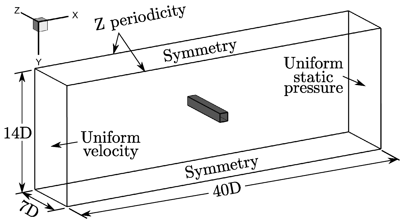
To reproduce the results of this experiment with CFD, only a fraction of the experimental lateral extent (9.75D) is considered with the use of periodic boundary conditions in order to reduce the computational cost. DDES simulations have been performed with three different computational domains with a spanwise length of , and . Since it has been observed that the level of velocity fluctuations in the near wake is greatly sensitive to the aspect ratio of the square cylinder up to a value of 7, the largest computational domain has been used as the nominal one and all the results presented in this paper have been obtained with this domain unless otherwise indicated. Note that the square cylinder is located in the center of the domain, as shown in Figure 1, and that the origin of the coordinate system is located at the center of the square cylinder. The distances that separate the square cylinder’s center from the inlet and from the outlet have been chosen based on two-dimensional URANS simulations making use of different domain sizes.
It is worth mentioning that a smaller domain size in the spanwise direction had been used for most of the simulations reported in the literature [14,15,16,18,19,20,21]. Two-point auto-correlations of the lateral velocity fluctuations along the lateral direction have been computed with the three different spanwise domain lengths (, and ). These auto-correlations showed that this specific velocity component is decorrelated over half the span only for the largest domain. The same procedure has been conducted by Garbaruk et al. [28] to validate their choice of four chord lengths in the spanwise direction for their DDES simulation of the flow around an airfoil at an angle of attack of 60. In order to further reduce the computational cost of the current simulations, symmetry boundary conditions (free-slip walls) are chosen to model the channel walls in the transversal direction. A uniform velocity and a turbulent viscosity ratio () of 0.01 are set at the inlet along with a uniform static pressure at the outlet.
The finite-volume open-source CFD toolbox OpenFOAM-2.1.x [29] is used to carry out the simulations. Both the URANS and DDES simulations are three-dimensional and make use of the same spatial and temporal resolutions for the sake of comparison. The choice of a three-dimensional domain for the URANS simulation stems from the fact that three-dimensional URANS simulations generally prove to be more reliable than their two-dimensional counterparts, even for the flow around two-dimensional geometries [4,24]. The convective fluxes are discretized with a second-order-accurate upwind scheme and all other discretization schemes are also second-order-accurate. The PISO algorithm handles the pressure-velocity coupling of the segregated solver that has been used [30]. Further, the residuals convergence criteria have been set to 1 × 10⁻⁵ for pressure, momentum and turbulent quantities. Simulations using a less restrictive criteria by an order of magnitude have showed only negligible differences.
The calculation grid corresponds to a two-dimensional unstructured mesh of 28,384 quad elements, as shown in Figure 2, which has been extruded in the spanwise direction resulting in a total of 3,973,760 cells. The grid spacing in the spanwise direction corresponds to the same spacing as the one used in the wake, where an almost constant spacing () of 0.05D in all three directions is used. The near-wall resolution gives rise to a dimensionless normal wall distance around one, while the streamwise and spanwise dimensionless wall distances are of the order of 100.
A time step of 0.01 has been chosen in order to obtain a Courant number of about 0.2 based on the upstream velocity in the wake’s refined region of the grid. This value is smaller than the one recommended by Spalart, who suggests that the Courant number should be around unity [31]. Mockett et al. [32] also demonstrated that a local Courant number below or equal to one is necessary in the region of the flow that is resolved in LES mode in order to obtain accurate results. This conclusion has been drawn from their study of the flow around a circular cylinder using a DDES approach [32]. A smaller Courant number of 0.2 based on the upstream velocity has been used in this study to account for the fact that the Courant number can locally reach higher values and to ensure the stability of the PISO algorithm. It is worth noting that the current time step is three times smaller than the finest one used by Mockett [32], which provides confidence that the numerical error associated with the temporal discretization should not be an issue. The time step used in the current study corresponds to roughly 750 time steps per shedding cycle. Simulations on finer grids ( and ) with smaller time steps ( and ) have been carried out by the authors in order to make sure that the conclusions of this study were independent of the resolution level that has been used to perform the simulations.
It is worth recalling that the boundary layers on the upstream face of the square cylinder are laminar and that the separation occurs at the two upstream sharp edges. The results of the DDES simulations should therefore not be affected by the RANS modeling in the attached boundary layers since no modeling is in fact needed in these laminar boundary layers. This allows focusing on the performances of the LES region of the DDES approach, as desired.
Because of the relatively low Reynolds number of this flow, some simulations have been carried out with a low-Reynolds-number correction as suggested by Spalart [6]. The correction has been implemented in the open-source computational fluid dynamics (CFD) toolbox OpenFOAM-2.1.x by the authors. With this correction, the ratio () is replaced with max() in the relation responsible for the near-wall viscous effects. The differences observed were negligible and the results presented in this paper have therefore been obtained without using this correction. In order to postprocess the results, every time signal has been decomposed into the sum of a time-averaged and a time-varying component. Applied to the streamwise velocity component, this results in the following decomposition:
where is the instantaneous signal, is the time-averaged component and is the time-varying component.
Lastly, all simulations have been initialized with a flow field obtained from a two-dimensional URANS simulation, and a minimum of 40 convective time units () was calculated in each simulation before recording any temporal signal for further statistical analysis. This time period corresponds to that required for the convection of one domain length based on the upstream velocity. Waiting 200 convective time units () before recording the temporal signals has also been tested, and it resulted in negligible differences. Sufficiently long time samples have been collected to ensure the statistical convergence of all the physical quantities of interest. The values of the time step () and the grid spacing in the wake region () along with the duration of the recorded time samples that have been chosen for the current study () are reported in Table 1.
3. Results and Discussion
3.1. Vortex Shedding
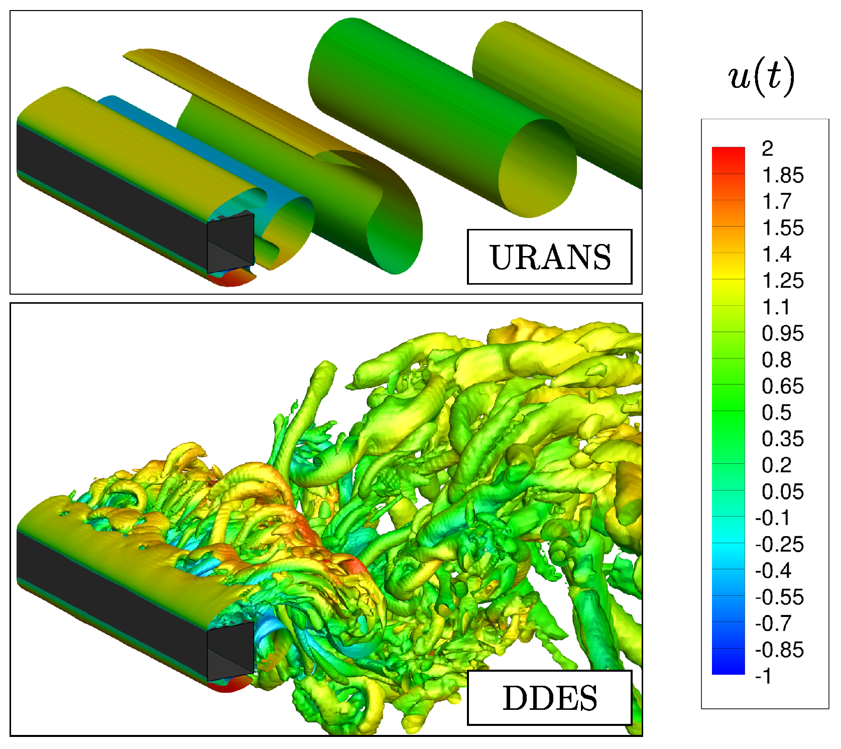
A qualitative comparison between the URANS and the DDES simulations is first conducted with respect to their vortex dynamics. The vortices are identified using the criterion proposed by Jeong and Hussain [33] for incompressible flows. One can observe in Figure 3 that the DDES simulation allows for the resolution of small-scale three-dimensional vortical structures while the URANS simulation provides in an essentially two-dimensional flow field without any visible three-dimensional instabilities in the shear layers, which is not representative of the reality of bluff-body wakes such as the circular cylinder case in the same range of Reynolds number [34]. This unrealistic behavior can be observed even if the URANS simulation is initialized with the flow field resulting from a DDES simulation. From this qualitative comparison, one can already expect that the level of velocity fluctuations should be smaller in the case of the URANS simulation compared to the DDES simulation, as will be demonstrated in the following sections.
3.2. Time-Averaged Velocity Component
For practical purposes, the averaged streamwise velocity component (), shown in Figure 4, is probably the most useful physical quantity to analyze in order to characterize the velocity recovery in a wake. The results shown in Figure 4 illustrate the good performance of the DDES approach in comparison to the URANS approach, which largely overestimates the velocity recovery. Indeed, the URANS simulation predicts an almost complete recovery of the upstream velocity only 6D downstream of the square cylinder’s center. One possible explanation of such a behavior is the very high eddy viscosity values that are predicted by the URANS simulation. Actually, the URANS simulation predicts a maximum value of the turbulent viscosity ratio () around 800 in the wake compared with a value of 20 for the DDES simulation. Breuer [25] has made similar observations with results obtained from simulations of the flow around an inclined flat plate in the same range of Reynolds numbers. High effective viscosity () values give rise to an increased transport of momentum which could explain the overestimation of the rate at which velocity is recovered in the URANS wake. Regarding the DDES simulation, the discrepancies observed in the near wake could be partly attributed to the overestimation of the transversal velocity fluctuations in this region as will further be discussed in Section 3.3. It is also interesting to note that the current results are in better agreement with the experimental data [13] than previous DES [21] and LES [14,15,16,19] simulations performed on this case. Indeed, most of these studies predicted a higher velocity recovery rate than the current DDES simulation. In the authors’ opinion, the main cause explaining this might be the use of an insufficient spatial resolution. In fact, a DDES simulation using a coarser resolution (not shown in this paper) has been carried out by the authors, and the results are found to be very similar to those of the aforementioned studies, i.e., showing a more pronounced overestimation of the velocity recovery rate.
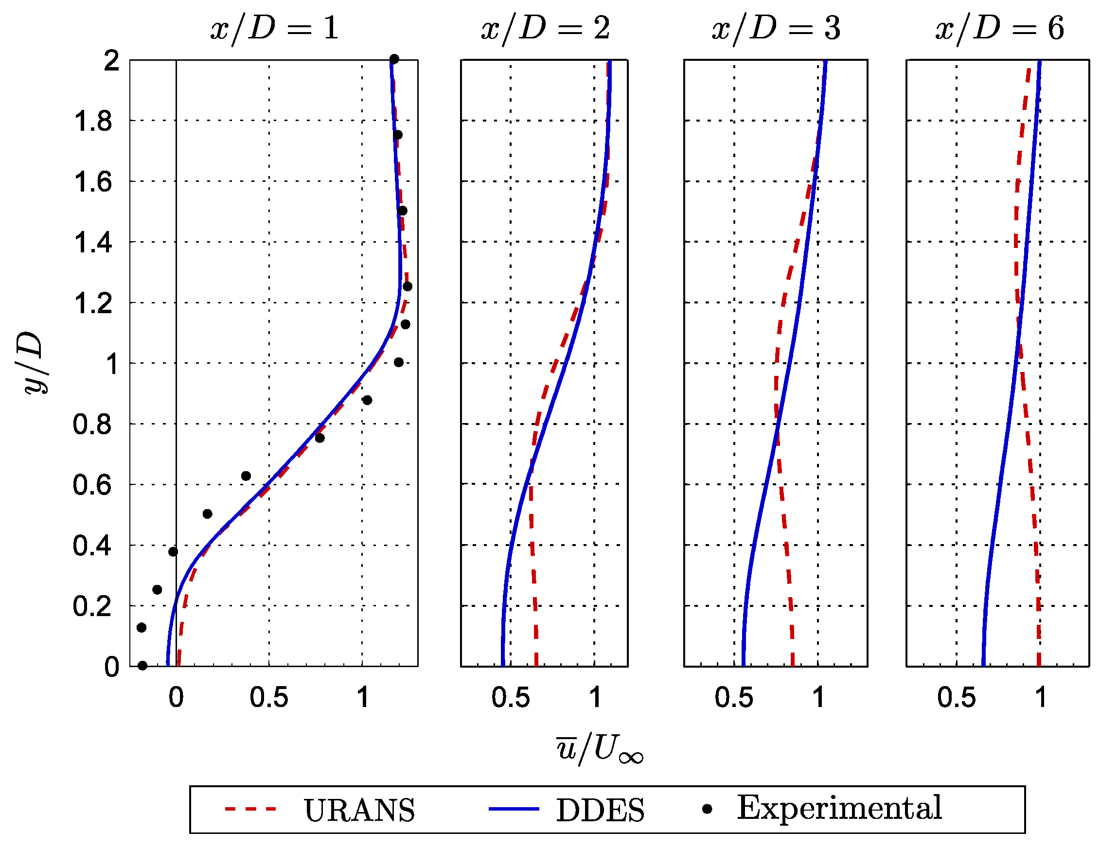
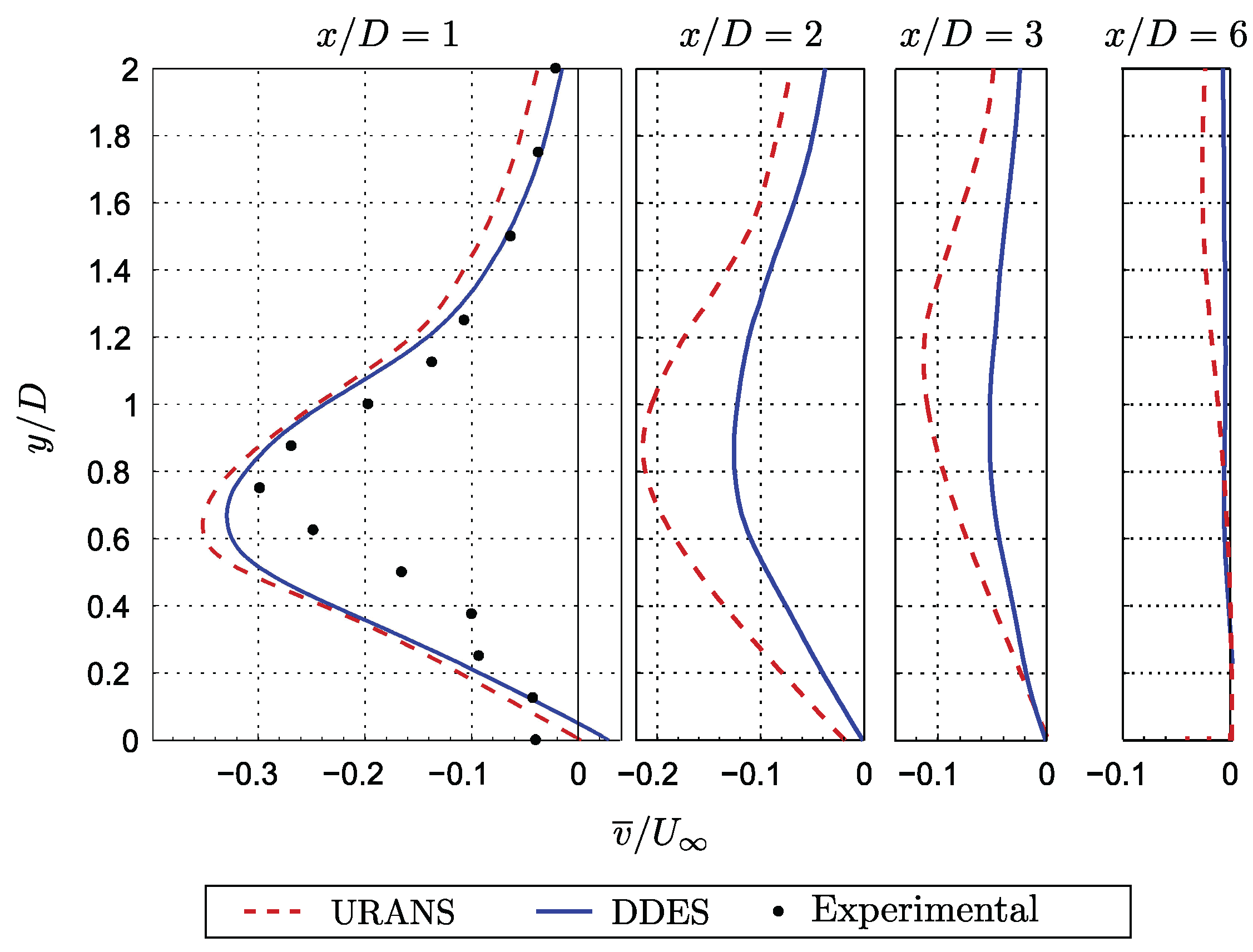
Numerical predictions of the averaged streamwise and transversal velocity profiles at several locations downstream of the square cylinder’s center are presented in Figure 5 and Figure 6, respectively. The URANS and the DDES simulations provide very similar predictions of the averaged velocity profiles at for both velocity components. At this location, it is observed in Figure 5 that both simulations overestimate the averaged streamwise velocity component in the wake’s center, as previously noted, and up to a distance of approximatively 0.7D in the transversal direction. The slightly underestimated averaged streamwise velocity component in the region between 0.7D and 1.3D is consistent with the overestimated velocity in the wake’s central region. Indeed, a smaller velocity deficit in the wake’s center is necessarily associated with an overestimation of the momentum transport across the wake, which is also responsible for a higher wake spreading rate. This is also consistent with the higher transversal velocities directed from outside the wake toward the wake’s central region (higher negative values) compared with the experimental data at this location. This can be observed on the left plot in Figure 6.
Nonetheless, even if the URANS and the DDES predictions of the averaged velocity profiles are very close to each other 1D downstream of the square cylinder’s center, large discrepancies are observed further downstream in Figure 5 and Figure 6. In the case of the averaged streamwise velocity profiles obtained with the URANS simulation, shown in Figure 5, a velocity deficit located away from the wake’s center is still observed even after the velocity in the wake’s center has been completely recovered. This is certainly not representative of a real wake’s behavior. Regarding the averaged profiles of the transversal velocity component shown in Figure 6, one can observe that the URANS simulation predicts higher negative values than the DDES simulation, except for the profile taken at 1D downstream. This observation is consistent with the higher recovery rate of the averaged streamwise velocity component obtained with the URANS simulation, as observed in Figure 4.
3.3. Time-Varying Velocity Component
It can be useful for engineering purposes, such as for determining the fatigue loads experienced by an object located in a wake, to know about the time-varying component of velocity. Furthermore, the time-varying component of velocity also provides an insight into the physics at play. It is therefore important to accurately predict the fluctuating components of velocity.
Fluctuations of the streamwise and transversal velocity components are compared with the experimental data [13] in Figure 7. As can be seen in Figure 7a, the level of streamwise velocity fluctuations predicted by the URANS simulation are underestimated while the DDES predictions are slightly overestimated over most of the studied area, the latter still being in good agreement with the experimental data. Regarding the transversal fluctuations, the URANS and DDES results are closer to each other than they are for the streamwise component. However, it is observed that DDES results are still more accurate, especially in the region of the wake located beyond 3D downstream of the square cylinder’s center.
It is interesting to note that both the URANS and the DDES simulations predict that the location where the highest transversal fluctuations are observed is closer behind the square cylinder than what is reported with the experimental data [13]. This same behavior has also been reported by previous DES simulations [21] and LES simulations [14,18,19] performed on the same case and is consistent with the smaller mean recirculation lengths () [34] predicted by these simulations and by the ones presented in the current paper. As pointed out by Celik et al. [35] in the case of LES simulations of free shear layers, this observation could be related to the difficulty of the subgrid-scale turbulence model to accurately predict the location of the laminar-turbulent transition in the free shear layers emerging from the two upstream sharp edges of the square cylinder. Also, it is interesting to note that the regions in the wake where the transversal fluctuations are overestimated correspond to the ones where the averaged streamwise velocity recovery rate is overestimated, and vice versa.
The lower level of fluctuations associated with the URANS modeling is related to the fact that the turbulence spectrum is essentially entirely modeled. Regarding the DDES simulation, the observed overestimation of the level of fluctuations is more surprising since only a part of the turbulence spectrum is resolved with a part of it being modeled. This same behavior has already been observed by other groups performing DES simulations of the same square cylinder case [20,21] and of a circular cylinder case [24]. However, these studies might have suffered from a too-narrow domain in the spanwise direction (4D and 2D respectively). Indeed, reducing the spanwise length of the domain from 7D to 5D and from 5D to 3D in previous simulations carried out by the authors has resulted in a continuous increase of the velocity fluctuation levels.
It is worth mentioning that there are also some results that have been reported in the literature [35,36,37,38] for which the resolved fraction of the turbulent kinetic energy that is predicted through a LES simulation is greater than the total amount of kinetic energy that is obtained with a direct numerical simulation (DNS), or even greater than the experimentally measured values. Among the possible causes, Celik et al. [35] have suggested that it might be attributed to a near-wall resolution that is too coarse. This leads to a deficiency in the amount of resolved eddies, which can contribute to a deterioration in the prediction of the strain rate. This, in turn, could possibly result in an underestimation of the dissipation, which would explain the overestimation of the turbulent kinetic energy for these cases.
A similar phenomenon can arise with the use of DES or DDES. When the attached boundary layers are modeled with a RANS approach, the modeled fraction of the turbulence spectrum in the RANS region does not allow the natural development of the instabilities that are required in the LES region. This gives rise to the existence of a transition zone, called the “gray area” [3,24], where the instabilities have not yet grown enough to compensate for the decrease in the amount of modeled eddies. Therefore, there is an analogy between a too coarse near-wall resolution in a LES simulation and the transition from a RANS to a LES modeling in a DES or a DDES simulation since both are characterized by a deficiency in the amount of resolved eddies.
However, the case chosen for the sake of the current study is not prone to being affected by this so-called “gray area” since the boundary layers on the upstream face of the square cylinder that separate at both upstream sharp edges are laminar. Consequently, the laminar-turbulent transition occurs in the separated shear layers where the LES approach of the DDES simulations is active.
3.4. Integral Flow Quantities
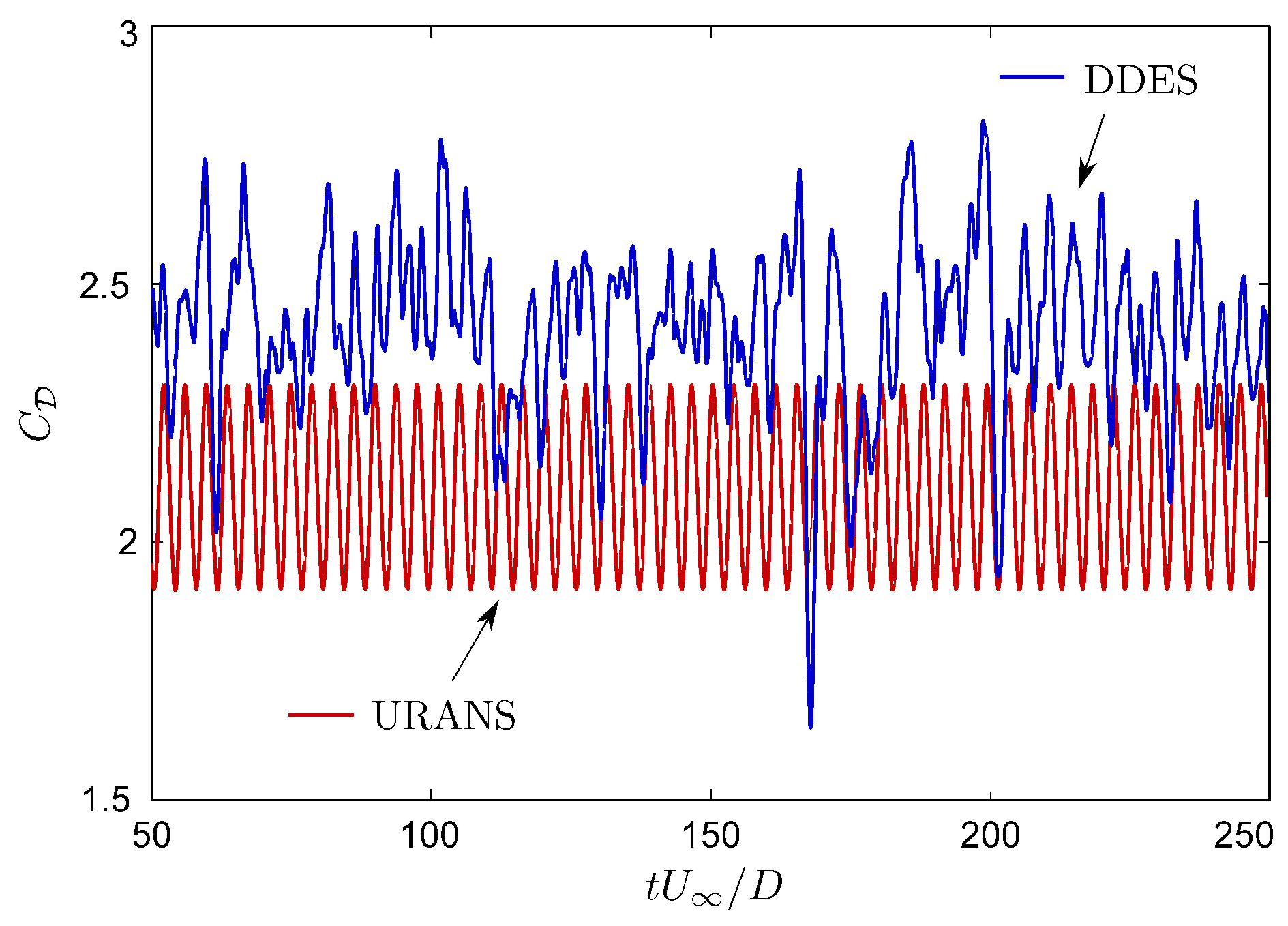
Samples of the drag coefficient temporal signal obtained with the URANS and the DDES simulations are shown in Figure 8. It is observed that the URANS drag signal is very similar to a sinusoidal wave while the DDES drag signal consists in the superposition of several modes. The same type of signal as the one obtained with the DDES simulation has already been observed in similar simulations around a circular cylinder [24] and a rectangular cylinder [39], and is more representative of real drag signals observed in the case of bluff-body flows [5].
The value of five different integral flow quantities obtained with the current study are reported in Table 2. The first quantity is the time-averaged drag coefficient ():
where is the drag force acting on the square cylinder, is the duration of the signal used to compute the average value (see Table 1), is the fluid density, is the freestream velocity and D is the cylinder’s width. The other integral quantities considered are the Strouhal number (), the mean recirculation length () defined as the distance in the wake where a zero mean streamwise velocity is reached, the root mean square (rms) of the drag coefficient fluctuations ():
and the rms of the lift coefficient fluctuations (), which is defined in a way similar to . Note that all the force coefficients are given in units per span length. For comparison purposes, values obtained from experimental measurements [13,40,41] and from DES [20,21] and LES [14,15,16,17,18,19] simulations performed by other research groups are also reported.
It is important to note that the procedure used by Lyn et al. [13] to determine is questionable, as mentioned by Sohankar et al. [19]. Indeed, their value has been obtained from the streamwise momentum flux at 8D downstream of the square cylinder’s center without taking into account the pressure field. In fact, a negative contribution from the streamwise momentum flux to the time-averaged drag coefficient has been observed with the simulations performed by Sohankar et al. [19] as well as with the simulations of the current study.
Moreover, Bearman and Obasaju [40] and Norberg [41] have performed experiments in similar cases in the same range of Reynolds numbers. Based on the results of these experiments, Sohankar et al. [19] reported a value of equal to 2.1 obtained by applying a correction in order to eliminate the blockage effects of these experiments. Regarding the experiment performed by Lyn et al. [13], the blockage effects should result in an increase in of approximatively 12%, according to Sohankar et al. [19]. This allows for modification of the corrected value reported by Sohankar et al. [19] in order to take into account the blockage effects corresponding to the channel size used in the experiment of Lyn et al. [13] for a straightforward comparison with the results of the current study. The resulting value of is equal to 2.35, as reported in Table 2, and is in good agreement with the value of 2.4 reported in Blevins’ handbook [42] for the same blockage and in the same range of Reynolds numbers.
It is observed that the value obtained with the current DDES simulation is closer to the value obtained in the experiments performed by Bearman and Obasaju [40] and by Norberg [41], after being corrected for the blockage effects of the current study, than the one obtained with the URANS simulation. Also, it is interesting to note the large variation in the values of predicted by other DES and LES simulations, thus suggesting that this physical quantity is very sensitive to the various flow parameters, as pointed out by Rodi et al. [15].
Regarding the Strouhal number, the value obtained with the URANS simulation is slightly closer to the experimental values than the one obtained with the DDES simulation. However, it is worth noting that the characteristics of the flow field predicted with the current DDES simulation are physically consistent. Indeed, a higher value of the time-averaged drag coefficient is generally associated with a smaller Strouhal number, a smaller mean recirculation length and larger velocity fluctuations in the near wake, as pointed out by Sohankar et al. [19] for the same case, and by Travin et al. [24] and Williamson [34] for the case of a circular cylinder. Lastly, the rms of the drag fluctuations and the lift fluctuations obtained from the DDES simulation agree with the values reported in the various studies that used a LES turbulence model. Moreover, it is observed that the size of the domain in the spanwise direction has a significant effect on the results, especially regarding . The fact that the spanwise domain length of the other simulations performed using DES in the literature was probably explains why the simulation with the smallest spanwise domain length () yields the best agreement with these results in terms of .
4. Conclusions and Outlook
Three-dimensional URANS and DDES simulations of the flow past a square cylinder (Re = 21,400) have been carried out with the open-source CFD toolbox OpenFOAM-2.1.x. The results have been compared with available experimental data [13] in order to assess the ability of DDES modeling at simulating a wake adequately. The Spalart–Allamaras turbulence model has been chosen for both modeling approaches.
The URANS simulation has yielded an essentially two-dimensional behavior, even if a three-dimensional grid with a spanwise length of 7D was used, and even after being initialized with the results of a DDES simulation. Large discrepancies have been observed between the URANS results and the experimental measurements [13], especially regarding the time-average and fluctuations of the streamwise velocity component. Unlike the URANS case, the DDES simulation exhibited a more realistic three-dimensional behavior. The agreement of the DDES results with the experimental data [13], regarding both the time-averaged and the time-varying components of velocity, has been similar or far superior to the URANS results, depending on the physical quantity that is considered.
A corrected value reported by Sohankar et al. [19], obtained from the experiments performed by Bearman and Obasaju [40] and Norberg [41], has been modified to take into account the blockage effects corresponding to the domain size used in the current study, according to the method proposed by Sohankar et al. [19]. The value obtained with the DDES simulation of the current study is in better agreement with this modified experimental value than the one obtained with the URANS simulation. On the other hand, a closer match with the experimental value of the Strouhal number has been observed with the URANS simulation.
The effect of the spanwise domain length has been found to have a considerable impact on the results, especially regarding the fluctuations of the drag coefficient. The fact that most of the previous studies on this benchmark case used a smaller domain size might partly explain the scatter observed between the results of the different numerical and experimental studies.
Based on the current study, it is concluded that DDES modeling appears as a good approach to reliably simulate wakes, especially far wakes of bluff bodies. Some unanswered questions remain regarding the effect of the “gray area” for flows involving turbulent boundary layers modeled in RANS mode as well as for flows for which the separations points are not dictated by the body geometry, namely flows around a body with no sharp edges. These important aspects of DDES simulations should be addressed in future studies.
Acknowledgments
Financial support from the Natural Sciences and Engineering Research Council of Canada (NSERC) and the Fonds de Recherche du Québec-Nature et Technologies (FRQNT) is gratefully acknowledged by the authors. Computations were performed on the Guillimin and Colosse supercomputers at the CLUMEQ HPC Consortium under the auspices of Compute Canada.
Author Contributions
Matthieu Boudreau and Jean-Christophe Veilleux developed the numerical methodology, Matthieu Boudreau and Guy Dumas analyzed the data, and Matthieu Boudreau wrote the paper.
Conflicts of Interest
The authors declare no conflict of interest. The founding sponsors had no role in the design of the study; in the collection, analyses, or interpretation of data; in the writing of the manuscript, and in the decision to publish the results.
Abbreviations
The following abbreviations are used in this manuscript:
| CFD | computational fluid dynamics |
| DDES | delayed detached-eddy simulation |
| DES | detached-eddy simulation |
| LES | large eddy simulation |
| RANS | Reynolds-averaged Navier–Stokes |
| rms | root mean square |
| URANS | unsteady Reynolds-averaged Navier–Stokes |
References
- Muscari, R.; Di Mascio, A.; Verzicco, R. Modeling of vortex dynamics in the wake of a marine propeller. Comput. Fluids 2013, 73, 65–79. [Google Scholar] [CrossRef]
- Spalart, P.R. Strategies for turbulence modelling and simulations. Int. J. Heat Fluid Flow 2000, 21, 252–263. [Google Scholar] [CrossRef]
- Spalart, P.R. Detached-Eddy Simulation. Annu. Rev. Fluid Mech. 2009, 41, 181–202. [Google Scholar] [CrossRef]
- Shur, M.; Spalart, P.R.; Squires, K.D.; Strelets, M.; Travin, A. Three Dimensionality in Reynolds-Averaged Navier-Stokes Solutions Around Two-Dimensional Geometries. AIAA J. 2005, 43, 1230–1242. [Google Scholar] [CrossRef]
- Najjar, F.; Balachandar, S. Low-frequency unsteadiness in the wake of a normal flat plate. J. Fluid Mech. 1998, 370, 101–147. [Google Scholar] [CrossRef]
- Spalart, P.R.; Deck, S.; Shur, M.L.; Squires, K.D.; Strelets, M.; Travin, A. A new version of detached-eddy simulation, resistant to ambiguous grid densities. Theor. Comput. Fluid Dyn. 2006, 20, 181–195. [Google Scholar] [CrossRef]
- Paik, J.; Sotiropoulos, F.; Porté-Agel, F. Detached eddy simulation of flow around two wall-mounted cubes in tandem. Int. J. Heat Fluid Flow 2009, 30, 286–305. [Google Scholar] [CrossRef]
- Nasif, G.; Barron, R.; Balachandar, R. DES evaluation of near-wake characteristics in a shallow flow. J. Fluids Struct. 2014, 45, 153–163. [Google Scholar] [CrossRef]
- Muld, T.W.; Efraimsson, G.; Henningson, D.S.; Herbst, A.H. Analysis of flow structures in the wake of a high-speed train. In The Aerodynamics of Heavy Vehicles III. Lecture Notes in Applied and Computational Mechanics; Springer: Cham, Switzerland, 2016; Volume 79, pp. 3–19. [Google Scholar]
- Felli, M.; Camussi, R.; Di Felice, F. Mechanisms of evolution of the propeller wake in the transition and far fields. J. Fluid Mech. 2011, 682, 5–53. [Google Scholar] [CrossRef] [Green Version]
- Boudreau, M.; Dumas, G. Comparison of the wake recovery of the axial-flow and cross-flow turbine concepts. J. Wind Eng. Ind. Aerodyn. 2017, 165, 137–152. [Google Scholar] [CrossRef]
- Wilcox, D. Turbulence Modeling for CFD, 2nd ed.; DCW Industries, Inc.: Flintridge, CA, USA, 1998. [Google Scholar]
- Lyn, D.A.; Einav, S.; Rodi, W.; Park, J.H. A laser-Doppler velocimetry study of ensemble-averaged characteristics of the turbulent near wake of a square cylinder. J. Fluid Mech. 1995, 304, 285–319. [Google Scholar] [CrossRef]
- Voke, P.R. Flow Past a Square Cylinder: Test Case LES2. In Direct and Large-Eddy Simulation II; ERCOFTAC Series; Chollet, J.P., Voke, P., Kleiser, L., Eds.; Springer: Dordrecht, The Netherlands, 1997; Volume 5, pp. 355–373. [Google Scholar]
- Rodi, W.; Ferziger, J.H.; Breuer, M.; Pourquiée, M. Status of Large Eddy Simulation: Results of a Workshop. J. Fluids Eng. 1997, 119, 248–262. [Google Scholar] [CrossRef]
- Fureby, C.; Tabor, G.; Weller, H.; Gosman, A. Large Eddy Simulations of the Flow Around a Square Prism. AIAA J. 2000, 38, 442–452. [Google Scholar] [CrossRef]
- Moussaed, C.; Wornom, S.; Salvetti, M.V.; Koobus, B.; Dervieux, A. Impact of dynamic subgrid-scale modeling in variational multiscale large-eddy simulation of bluff-body flows. Acta Mech. 2014, 225, 3309–3323. [Google Scholar] [CrossRef]
- Schmidt, S. Grobstruktursimulation Turbulenter Strömungen in Komplexen Geometrien und bei Hohen Reynoldszahlen; Mensch Mensch & Buch-Verlag: Berlin, Germany, 2000. [Google Scholar]
- Sohankar, A.; Norberg, C.; Davidson, L. Large Eddy Simulation of Flow Past a Square Cylinder: Comparison of Different Subgrid Scale Models. J. Fluids Eng. 2000, 122, 39–47. [Google Scholar] [CrossRef]
- Barone, M.; Roy, C. Evaluation of Detached Eddy Simulation for Turbulent Wake Applications. AIAA J. 2006, 44, 3062–3071. [Google Scholar] [CrossRef]
- Schmidt, S.; Thiele, F. Comparison of numerical methods applied to the flow over wall-mounted cubes. Int. J. Heat Fluid Flow 2002, 23, 330–339. [Google Scholar] [CrossRef]
- Pope, S. Turbulent Flows; Cambridge University Press: Cambridge, UK, 2000. [Google Scholar]
- Spalart, P.R.; Allmaras, S.R. One-Equation Turbulence Model for Aerodynamic Flows. La Recherche Aérospatiale 1994, 1, 5–21. [Google Scholar]
- Travin, A.; Shur, M.; Strelets, M.; Spalart, P.R. Detached-Eddy Simulations Past a Circular Cylinder. Flow Turbul. Combust. 2000, 63, 293–313. [Google Scholar] [CrossRef]
- Breuer, M.; Jovicic, N.; Mazaev, K. Comparison of DES, RANS and LES for the separated flow around a flat plate at high incidence. Int. J. Numer. Methods Fluids 2003, 41, 357–388. [Google Scholar] [CrossRef]
- Shur, M.; Spalart, P.R.; Strelets, M.; Travin, A. Detached-eddy simulation of an airfoil at high angle of attack. Eng. Turbul. Model. Exp. 1999, 4, 669–678. [Google Scholar]
- Spalart, P.R.; Jou, W.; Strelets, M.; Allmaras, S. Comments on the Feasibility of LES for Wings, and on a Hybrid RANS/LES Approach. In Proceedings of the International Conference on DNS/LES, Ruston, LA, USA, 4–8 August 1997. [Google Scholar]
- Garbaruk, A.; Leicher, S.; Mockett, C.; Spalart, P.R.; Strelets, M.; Thiele, F. Evaluation of time sample and span size effects in DES of nominally 2D airfoils beyond stall. Notes on Numerical Fluid Mechanics and Multidisciplinary Design. In Progress in Hybrid RANS-LES Modelling; Springer: Berlin/Heidelberg, Germany, 2010; Volume 111, pp. 87–99. [Google Scholar]
- OpenCFD. OpenFOAM-The Open Source CFD Toolbox—User’s Guide, 2.1 ed.; OpenCFD Ltd.: London, UK, 2012. [Google Scholar]
- Ferziger, J.H.; Perić, M. Computational Methods for Fluid Dynamics; Springer: Berlin/Heidelberg, Germany, 2002. [Google Scholar]
- Spalart, P.R. Young-Person’s Guide to Detached-Eddy Simulation Grids; Technical Report; NASA Technical Reports Server: Hampton, VA, USA, 2001.
- Mockett, C.; Perrin, R.; Reimann, T.; Braza, M.; Thiele, F. Analysis of Detached-Eddy Simulation for the Flow Around a Circular Cylinder with Reference to PIV Data. Flow Turbul. Combust. 2010, 85, 167–180. [Google Scholar] [CrossRef]
- Jeong, J.; Hussain, F. On the identification of a vortex. J. Fluid Mech. 1995, 285, 69–94. [Google Scholar] [CrossRef]
- Williamson, C.H.K. Vortex Dynamics in the Cylinder Wake. Annu. Rev. Fluid Mech. 1996, 28, 477–539. [Google Scholar] [CrossRef]
- Celik, I.; Cehreli, Z.; Yavuz, I. Index of Resolution Quality for Large Eddy Simulations. J. Fluids Eng. Trans. ASME 2005, 127, 949–958. [Google Scholar] [CrossRef]
- Gousseau, P.; Blocken, B.; Van Heijst, G.J.F. Quality assessment of Large-Eddy Simulation of wind flow around a high-rise building: Validation and solution verification. Comput. Fluids 2013, 79, 120–133. [Google Scholar] [CrossRef]
- Klein, M. An Attempt to Assess the Quality of Large Eddy Simulations in the Context of Implicit Filtering. Flow Turbul. Combust. 2005, 75, 131–147. [Google Scholar] [CrossRef]
- Meyers, J.; Geurts, B.J.; Baelmans, M. Database analysis of errors in large-eddy simulation. Phys. Fluids 2003, 15, 2740–2755. [Google Scholar] [CrossRef] [Green Version]
- Mannini, C.; Šoda, A.; Schewe, G. Numerical investigation on the three-dimensional unsteady flow past a 5:1 rectangular cylinder. J. Wind Eng. Ind. Aerodyn. 2011, 99, 469–482. [Google Scholar] [CrossRef]
- Bearman, P.; Obasaju, E. An Experimental Study of Pressure Fluctuations on Fixed and Oscillating Square-Section Cylinders. J. Fluid Mech. 1982, 119, 297–321. [Google Scholar] [CrossRef]
- Norberg, C. Flow around rectangular cylinders: Pressure forces and wake frequencies. J. Wind Eng. Ind. Aerodyn. 1993, 49, 187–196. [Google Scholar] [CrossRef]
- Blevins, R. Applied Fluid Dynamics Handbook; Krieger Publishing Company: Malabar, FL, USA, 1992. [Google Scholar]
Figure 1.
Domain and boundary conditions.

Figure 2.
Two-dimensional mesh (28,384 quad elements, ) which has been extruded in the spanwise direction to obtain the three-dimensional grid (3,973,760 cells).
Figure 2.
Two-dimensional mesh (28,384 quad elements, ) which has been extruded in the spanwise direction to obtain the three-dimensional grid (3,973,760 cells).
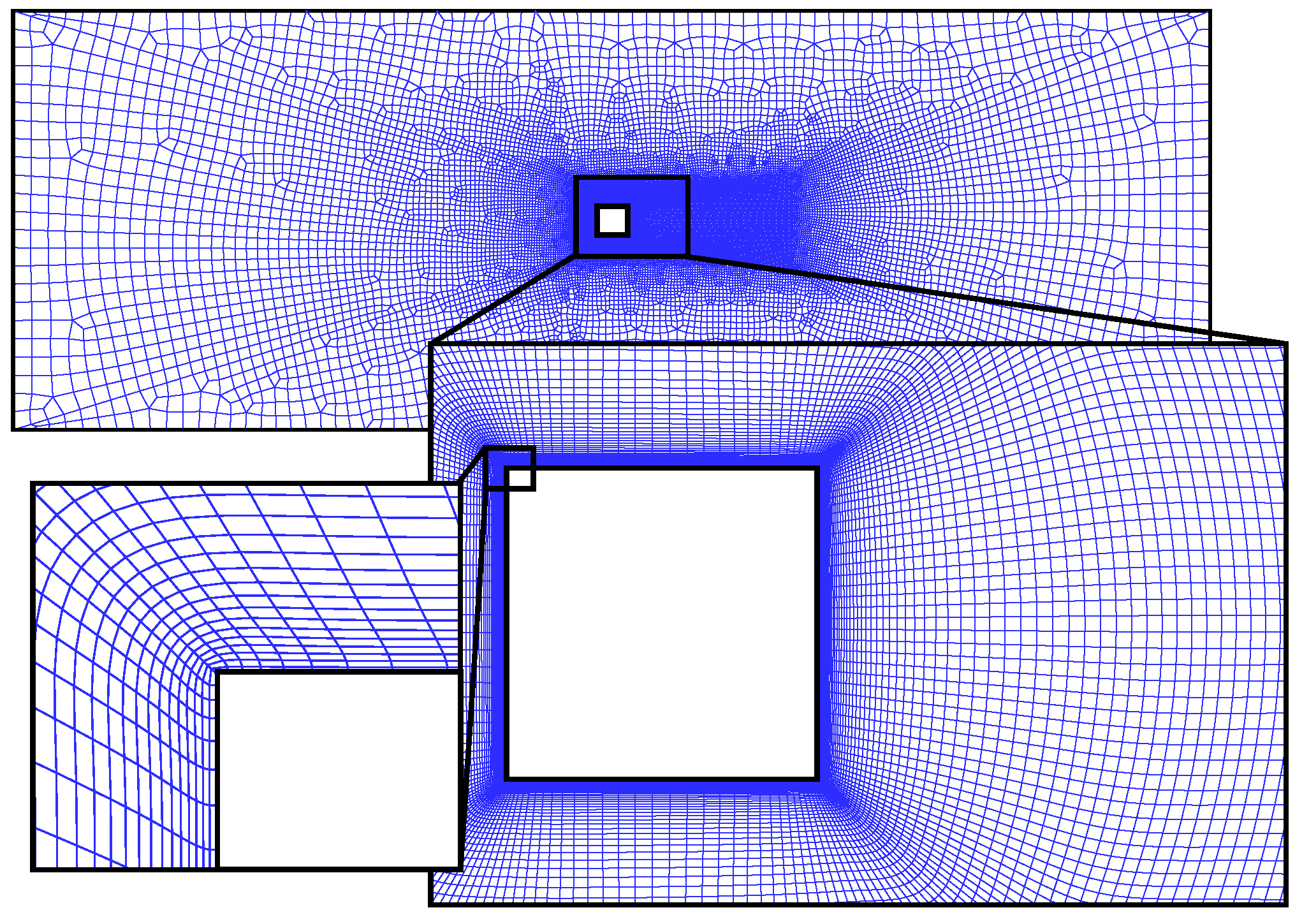
Figure 3.
Isosurfaces of the criterion for the unsteady Reynolds-averaged Navier–Stokes (URANS) (top) and the delayed detached-eddy simulation (DDES) simulations (bottom) colored by the instantaneous streamwise velocity component.
Figure 3.
Isosurfaces of the criterion for the unsteady Reynolds-averaged Navier–Stokes (URANS) (top) and the delayed detached-eddy simulation (DDES) simulations (bottom) colored by the instantaneous streamwise velocity component.

Figure 4.
Evolution of the averaged streamwise velocity component normalized with the upstream velocity () in the center of a square cylinder’s wake () compared with the experimental data [13].
Figure 4.
Evolution of the averaged streamwise velocity component normalized with the upstream velocity () in the center of a square cylinder’s wake () compared with the experimental data [13].
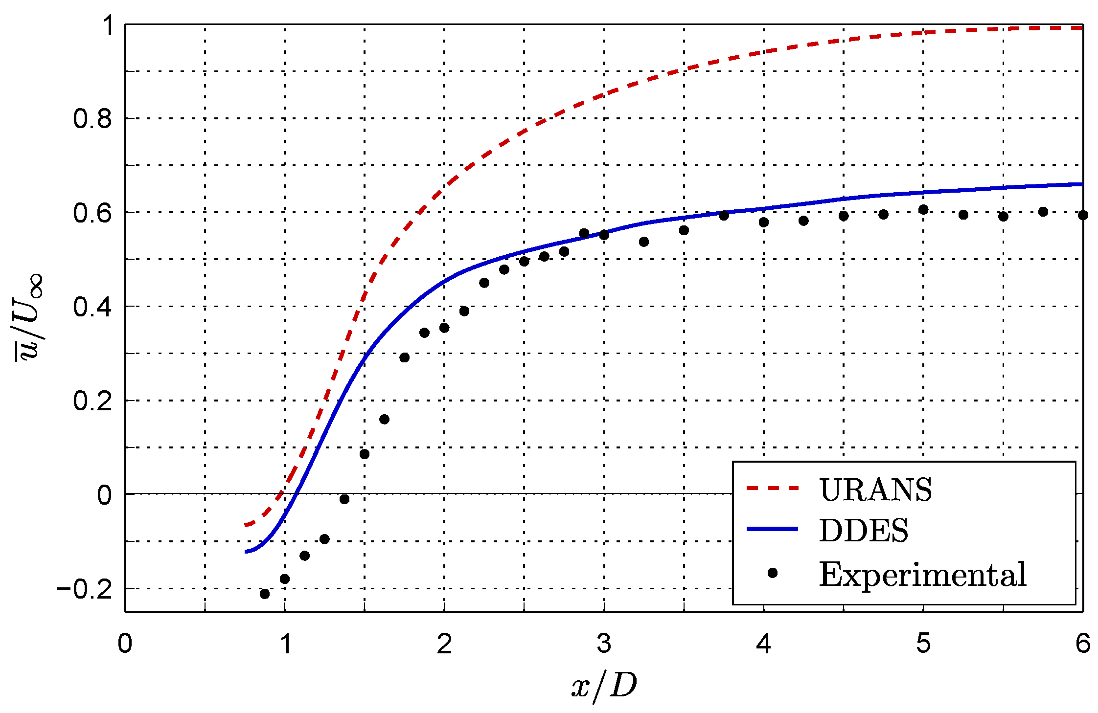
Figure 5.
Profiles of the averaged streamwise velocity component along the y-axis normalized with the upstream velocity () at several locations downstream of the square cylinder’s center compared with the experimental data [13].
Figure 5.
Profiles of the averaged streamwise velocity component along the y-axis normalized with the upstream velocity () at several locations downstream of the square cylinder’s center compared with the experimental data [13].

Figure 6.
Profiles of the averaged transversal velocity component along the y-axis normalized with the upstream velocity () at several locations downstream of the square cylinder’s center compared with the experimental data [13].
Figure 6.
Profiles of the averaged transversal velocity component along the y-axis normalized with the upstream velocity () at several locations downstream of the square cylinder’s center compared with the experimental data [13].

Figure 7.
Evolution of the root mean square (rms) of the velocity fluctuations normalized with the upstream velocity () in the center of a square cylinder’s wake () compared with the experimental data [13]. (a) Streamwise velocity fluctuations; (b) Transversal velocity fluctuations.
Figure 7.
Evolution of the root mean square (rms) of the velocity fluctuations normalized with the upstream velocity () in the center of a square cylinder’s wake () compared with the experimental data [13]. (a) Streamwise velocity fluctuations; (b) Transversal velocity fluctuations.
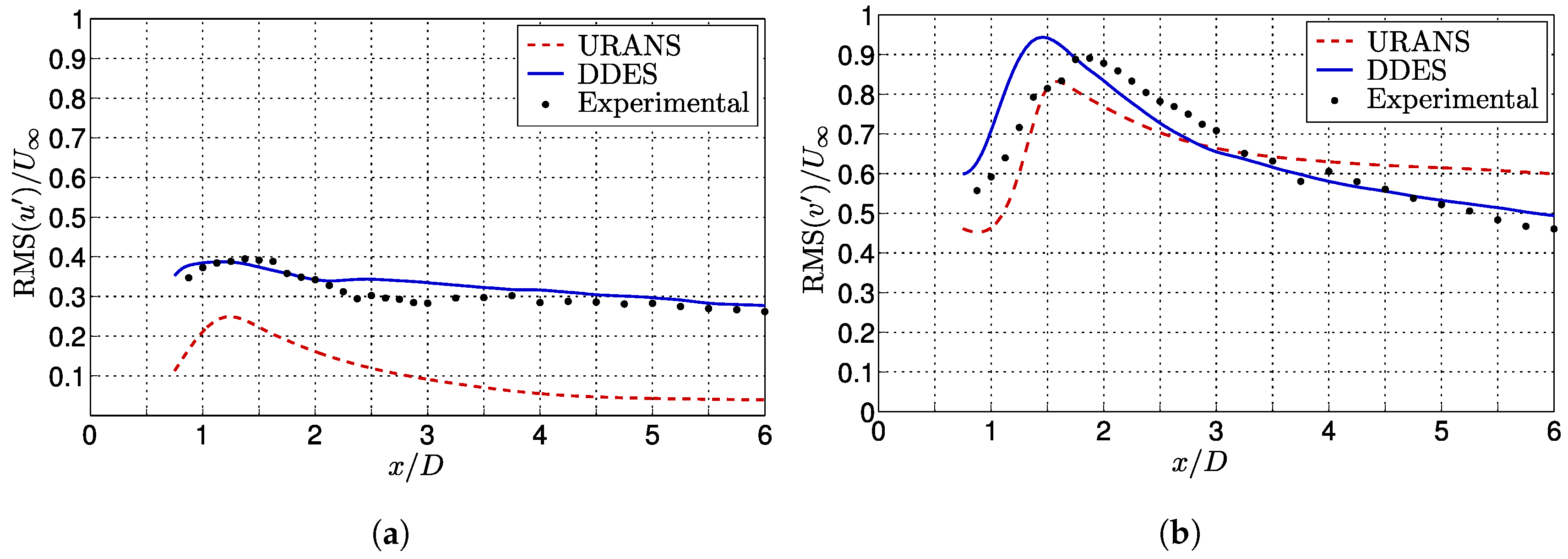
Figure 8.
Sample of the drag coefficient () temporal signals obtained with the URANS simulation (red) and the DDES simulation (blue).
Figure 8.
Sample of the drag coefficient () temporal signals obtained with the URANS simulation (red) and the DDES simulation (blue).


Table 1.
Values of the grid spacing in the wake region (), the time step (), and the duration of the time samples recorded for statistical analysis ().
Table 1.
Values of the grid spacing in the wake region (), the time step (), and the duration of the time samples recorded for statistical analysis ().
| Case | |||
|---|---|---|---|
| URANS | 0.05 | 0.01 | 209.5 |
| DDES | 0.05 | 0.01 | 1507.5 |
Table 2.
Comparison of the time-averaged drag coefficient (), the Strouhal number (), the mean recirculation length (), the rms of the drag coefficient fluctuations () and the rms of the lift coefficient fluctuations (). The results of the DDES simulations performed with three different aspect ratios (AR) are presented.
| Source | AR | |||||
|---|---|---|---|---|---|---|
| Current study | ||||||
| URANS | 7 | 2.11 | 0.133 | 0.97 | 0.14 | 1.56 |
| DDES | 3 | 2.36 | 0.123 | 1.20 | 0.26 | 1.50 |
| DDES | 5 | 2.40 | 0.126 | 1.15 | 0.21 | 1.51 |
| DDES | 7 | 2.41 | 0.126 | 1.07 | 0.17 | 1.47 |
| DES simulations | ||||||
| Barone/Roy [20] | 4 | 2.36 * | 0.131 * | 1.42 | 0.29 * | 1.30 * |
| Schmidt/Thiele [21] | 4 | 2.42 | 0.13 | 1.16 | 0.28 | 1.55 |
| LES simulations | ||||||
| Fureby et al. [16] | 8 | 2.0–2.2 | 0.129–0.135 | 1.23–1.37 | 0.17–0.20 | 1.30–1.34 |
| Moussaed et al. [17] | 2.06 | 0.128 | ≈1.3 | 0.24 | 1.28 | |
| Schmidt [18] | 4 | 2.18 | 0.13 | 1.07 | 0.19 | 1.47 |
| Sohankar et al. [19] | 4 | 2.03–2.32 | 0.126–0.132 | ≈1 | 0.16–0.20 | 1.23–1.54 |
| Rodi et al. [15] | 4 | 1.86–2.77 | 0.09–0.15 | 0.89–2.96 | 0.10–0.27 | 0.38–1.79 |
| Voke [14] | 4 | 2.03–2.79 | 0.13–0.16 | 1.02–1.61 | 0.12–0.36 | 1.01–1.68 |
| Experiments | ||||||
| Bearman/Obasaju [40] | 17 | 2.35 * | 0.135 * | - | - | 1.34 |
| Lyn et al. [13] | 9.75 | 2.1 | 0.132 | 1.38 | - | - |
| Norberg [41] | 51 | 2.35 * | 0.135 * | - | - | - |
© 2017 by the authors. Licensee MDPI, Basel, Switzerland. This article is an open access article distributed under the terms and conditions of the Creative Commons Attribution (CC BY) license (http://creativecommons.org/licenses/by/4.0/).
Share and Cite
MDPI and ACS Style
Boudreau, M.; Dumas, G.; Veilleux, J.-C. Assessing the Ability of the DDES Turbulence Modeling Approach to Simulate the Wake of a Bluff Body. Aerospace 2017, 4, 41. https://doi.org/10.3390/aerospace4030041
AMA Style
Boudreau M, Dumas G, Veilleux J-C. Assessing the Ability of the DDES Turbulence Modeling Approach to Simulate the Wake of a Bluff Body. Aerospace. 2017; 4(3):41. https://doi.org/10.3390/aerospace4030041
Chicago/Turabian StyleBoudreau, Matthieu, Guy Dumas, and Jean-Christophe Veilleux. 2017. "Assessing the Ability of the DDES Turbulence Modeling Approach to Simulate the Wake of a Bluff Body" Aerospace 4, no. 3: 41. https://doi.org/10.3390/aerospace4030041
Note that from the first issue of 2016, this journal uses article numbers instead of page numbers. See further details here.