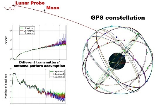
Figure 1.
Elevation angle of the global positioning system (GPS) antenna pattern from which the signals are received, for the assumed moon transfer orbit (MTO) in
Section 2.1.
Figure 1.
Elevation angle of the global positioning system (GPS) antenna pattern from which the signals are received, for the assumed moon transfer orbit (MTO) in
Section 2.1.
Figure 2.
Number of GPS satellites received from main and side lobes of the transmitters’ antenna pattern, for the assumed MTO in
Section 2.1.
Figure 2.
Number of GPS satellites received from main and side lobes of the transmitters’ antenna pattern, for the assumed MTO in
Section 2.1.
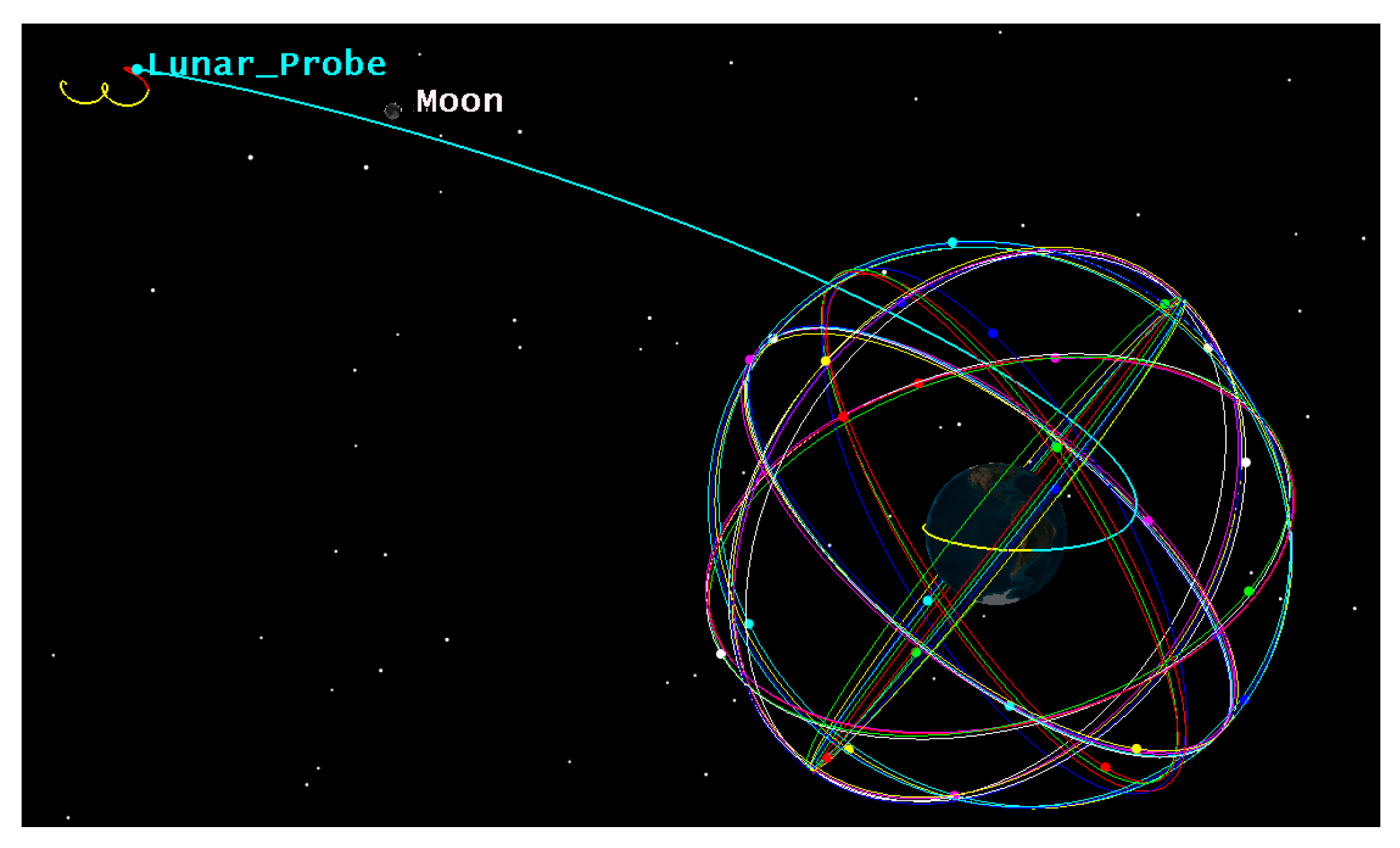
Figure 3.
Assumed MTO for the receiver.
Figure 3.
Assumed MTO for the receiver.
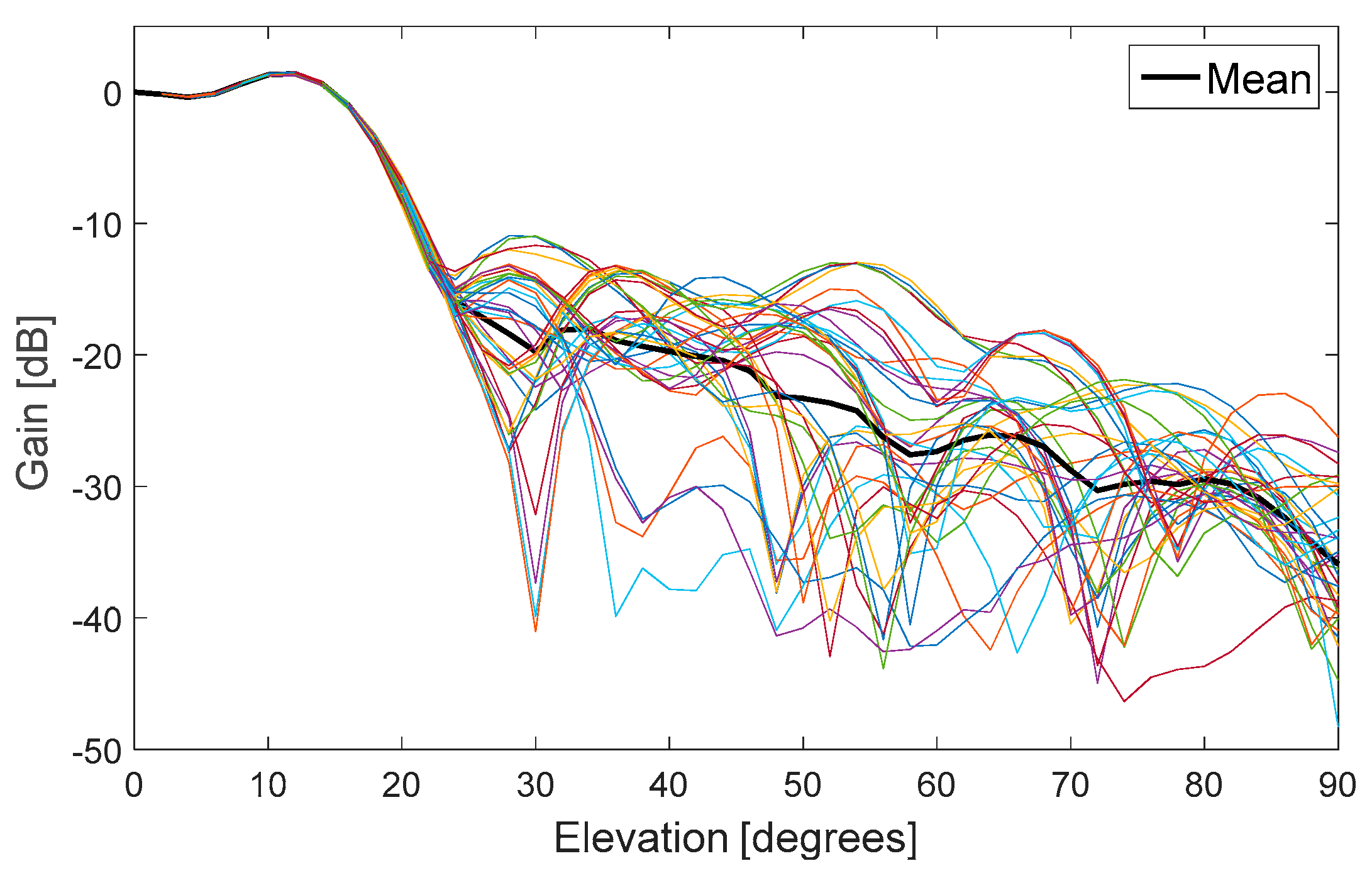
Figure 4.
Block IIF GPS L1 antenna gain pattern.
Figure 4.
Block IIF GPS L1 antenna gain pattern.
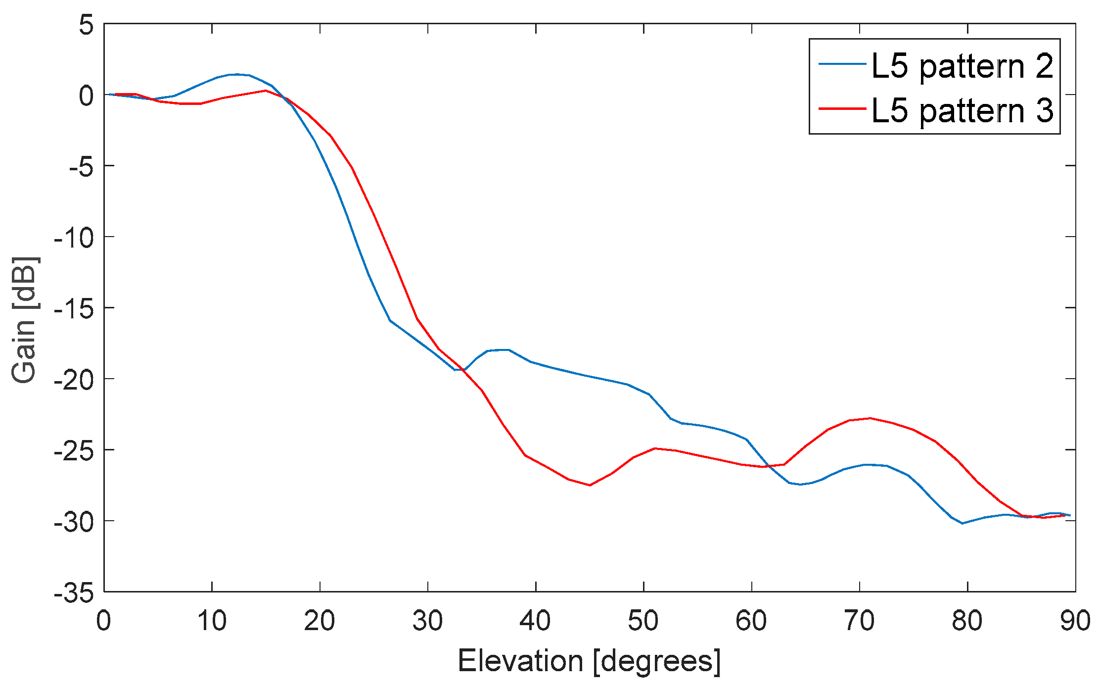
Figure 5.
GPS L5 antenna gain pattern.
Figure 5.
GPS L5 antenna gain pattern.
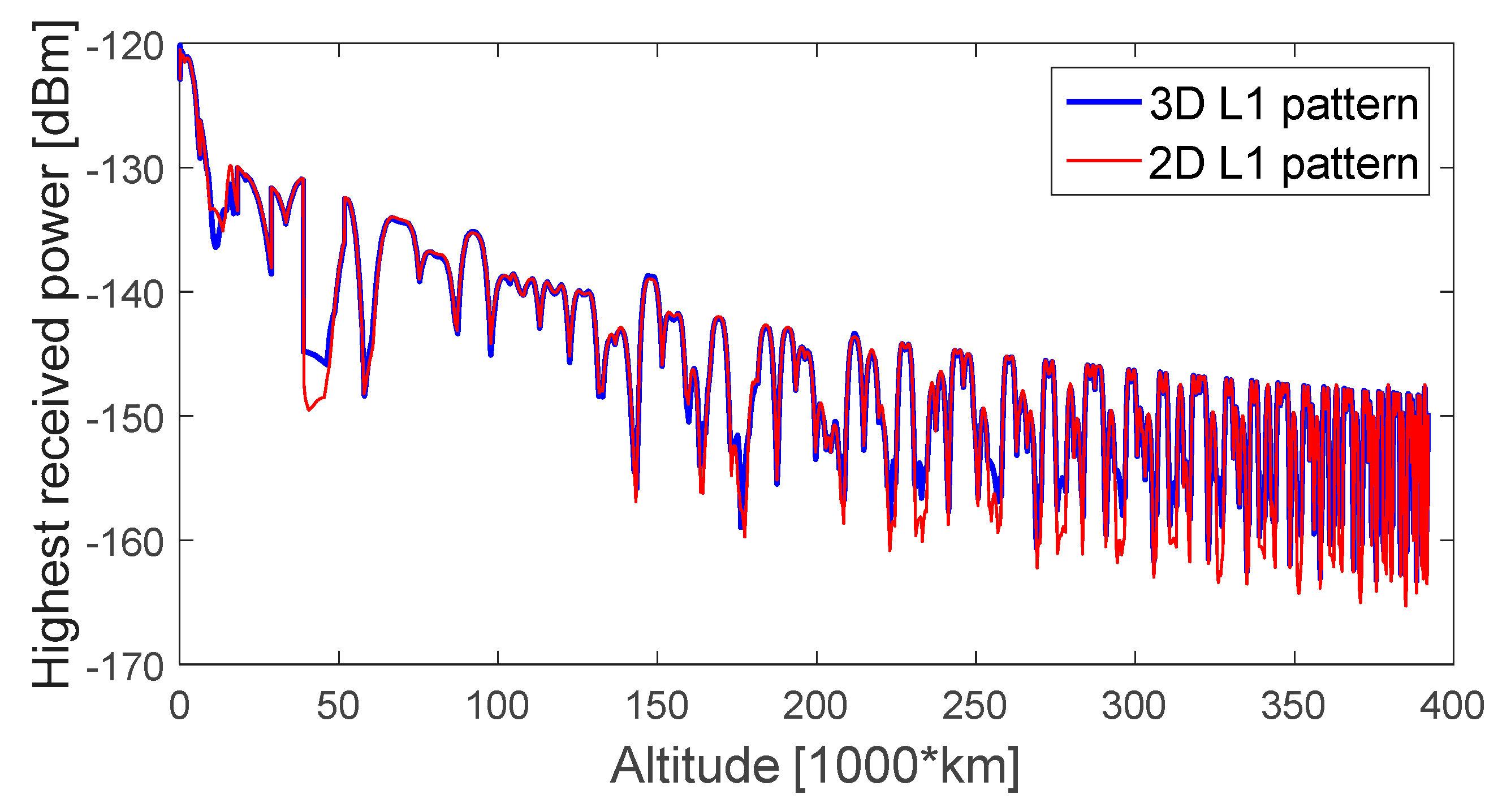
Figure 6.
Highest received power level of GPS L1 signals, during the considered MTO, for a 0 dBi receiver gain pattern.
Figure 6.
Highest received power level of GPS L1 signals, during the considered MTO, for a 0 dBi receiver gain pattern.
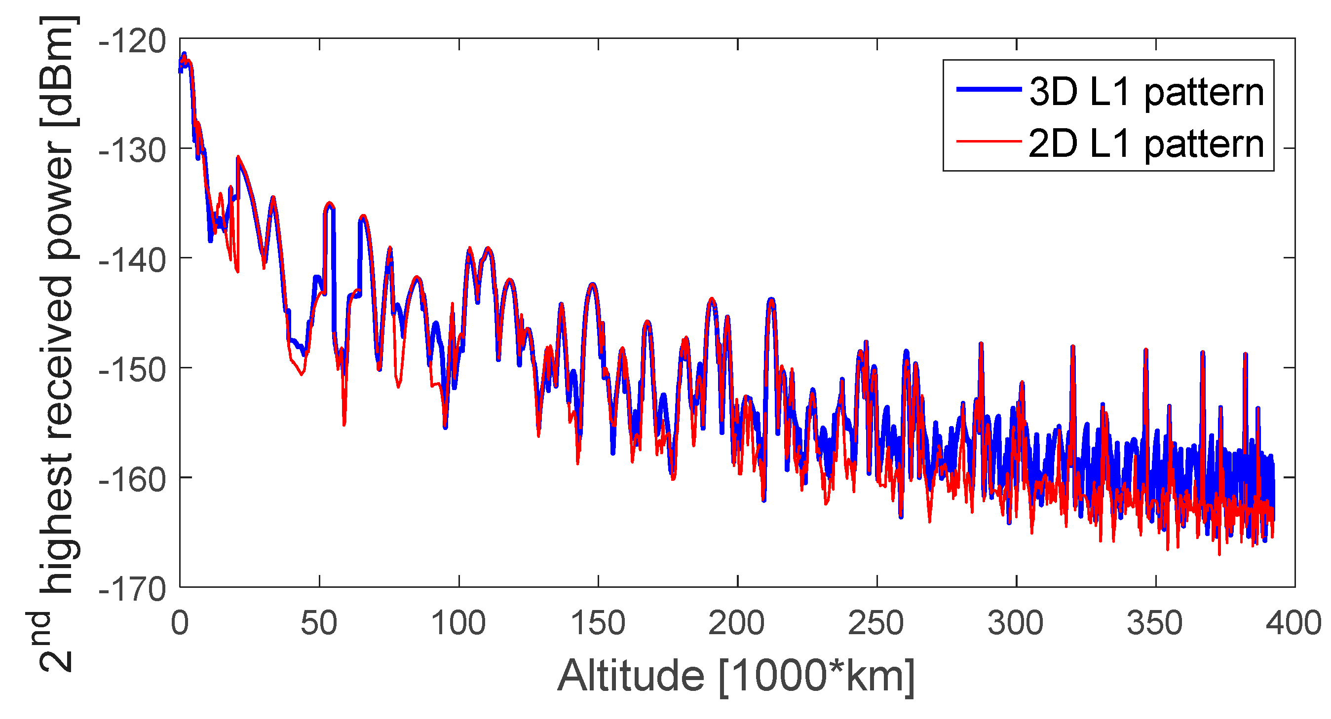
Figure 7.
Second-highest received power level of GPS L1 signals, during the considered MTO, for a 0 dBi receiver gain pattern.
Figure 7.
Second-highest received power level of GPS L1 signals, during the considered MTO, for a 0 dBi receiver gain pattern.
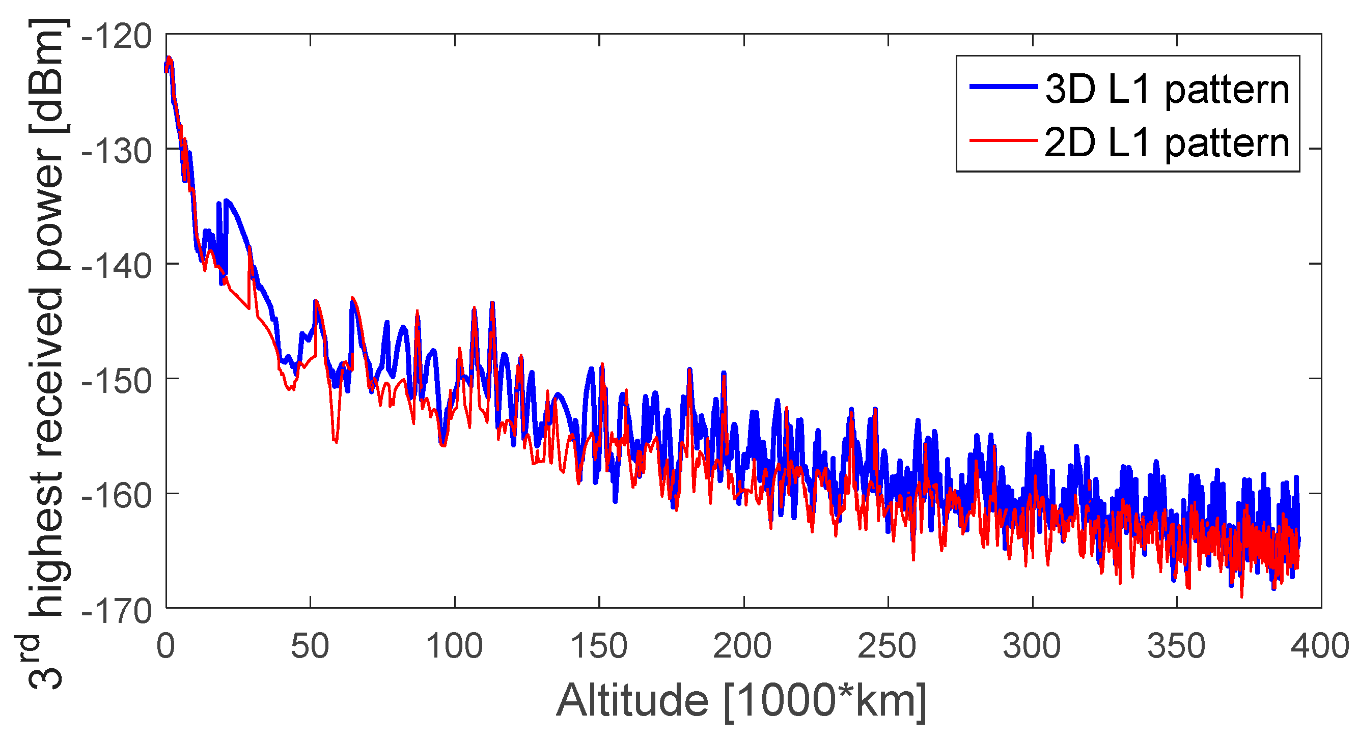
Figure 8.
Third-highest received power level of GPS L1 signals, during the considered MTO, for a 0 dBi receiver gain pattern.
Figure 8.
Third-highest received power level of GPS L1 signals, during the considered MTO, for a 0 dBi receiver gain pattern.
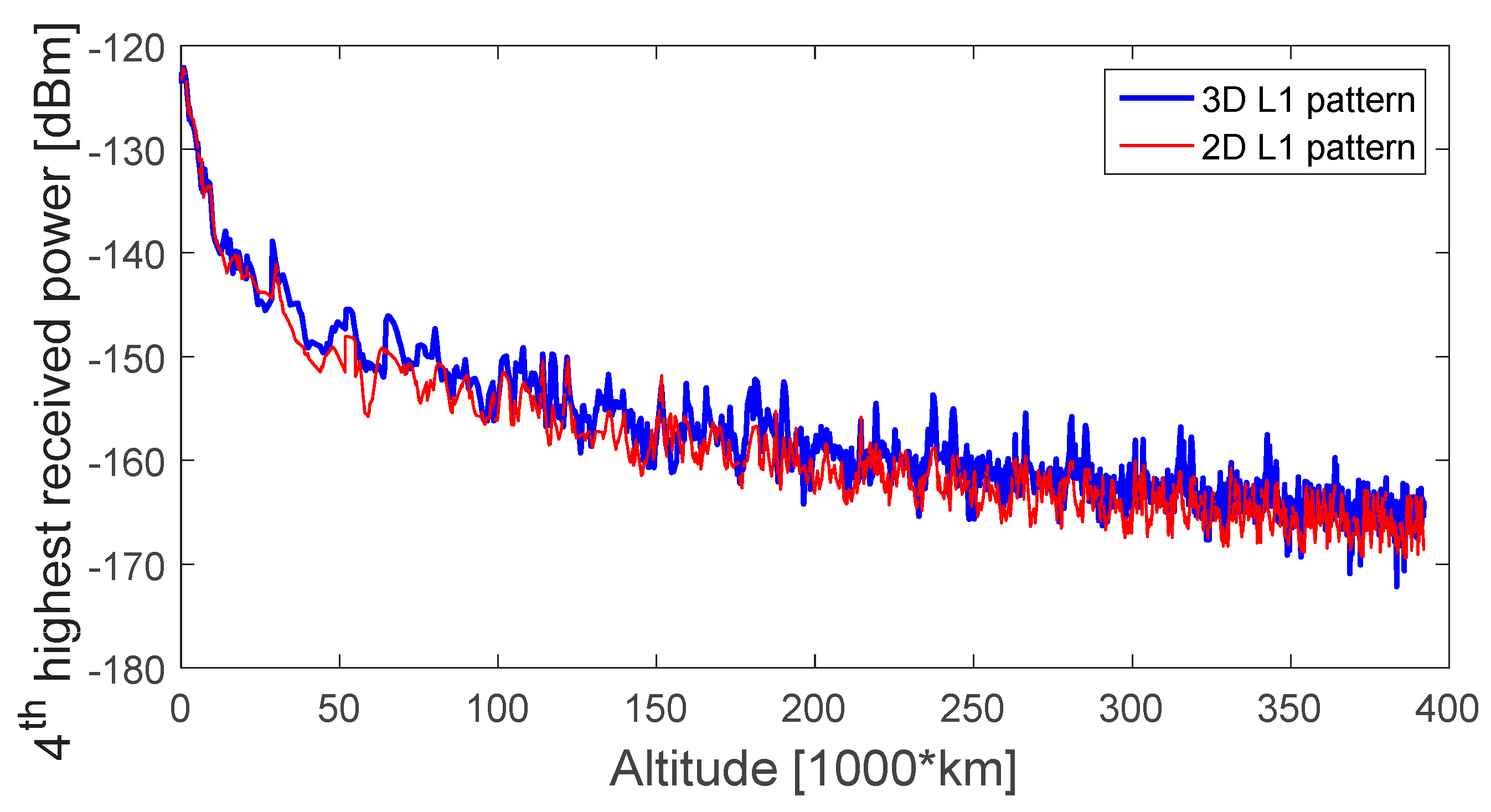
Figure 9.
Fourth-highest received power level of GPS L1 signals, during the considered MTO, for a 0 dBi receiver gain pattern.
Figure 9.
Fourth-highest received power level of GPS L1 signals, during the considered MTO, for a 0 dBi receiver gain pattern.
Figure 10.
Available GPS L1 signals, during the assumed MTO, for a 10 dBi receiver gain pattern.
Figure 10.
Available GPS L1 signals, during the assumed MTO, for a 10 dBi receiver gain pattern.
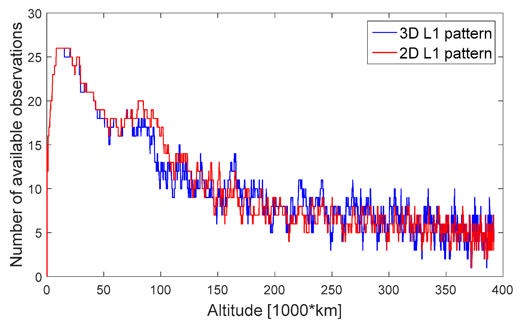
Figure 11.
Number of available observations during the assumed MTO.
Figure 11.
Number of available observations during the assumed MTO.
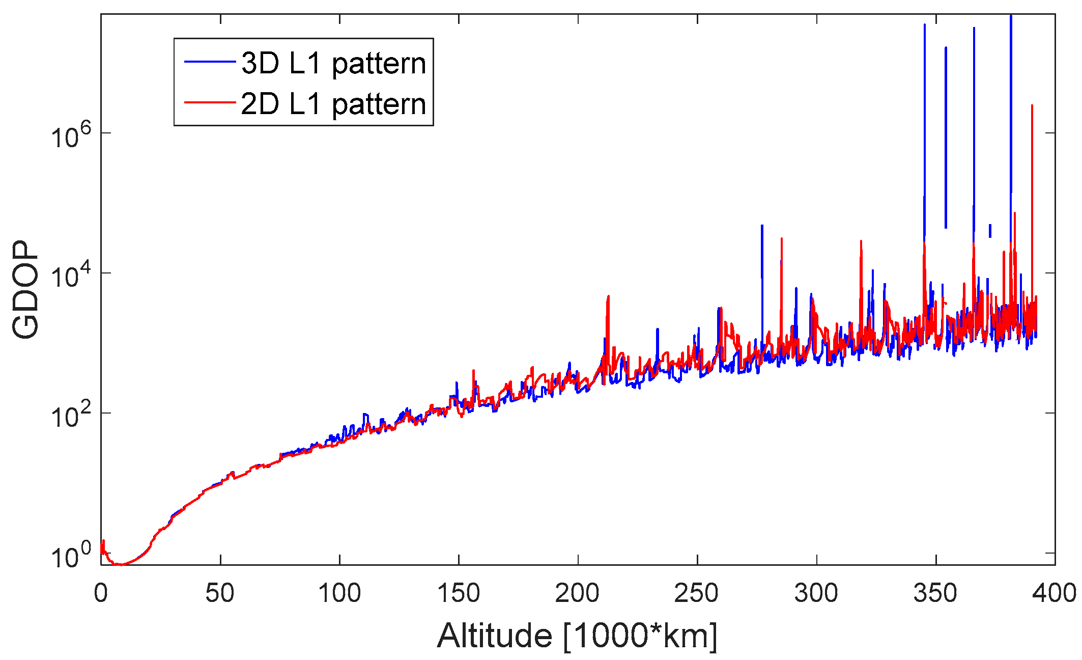
Figure 12.
Geometric dilution of precision (GDOP) in log scale during the assumed MTO.
Figure 12.
Geometric dilution of precision (GDOP) in log scale during the assumed MTO.
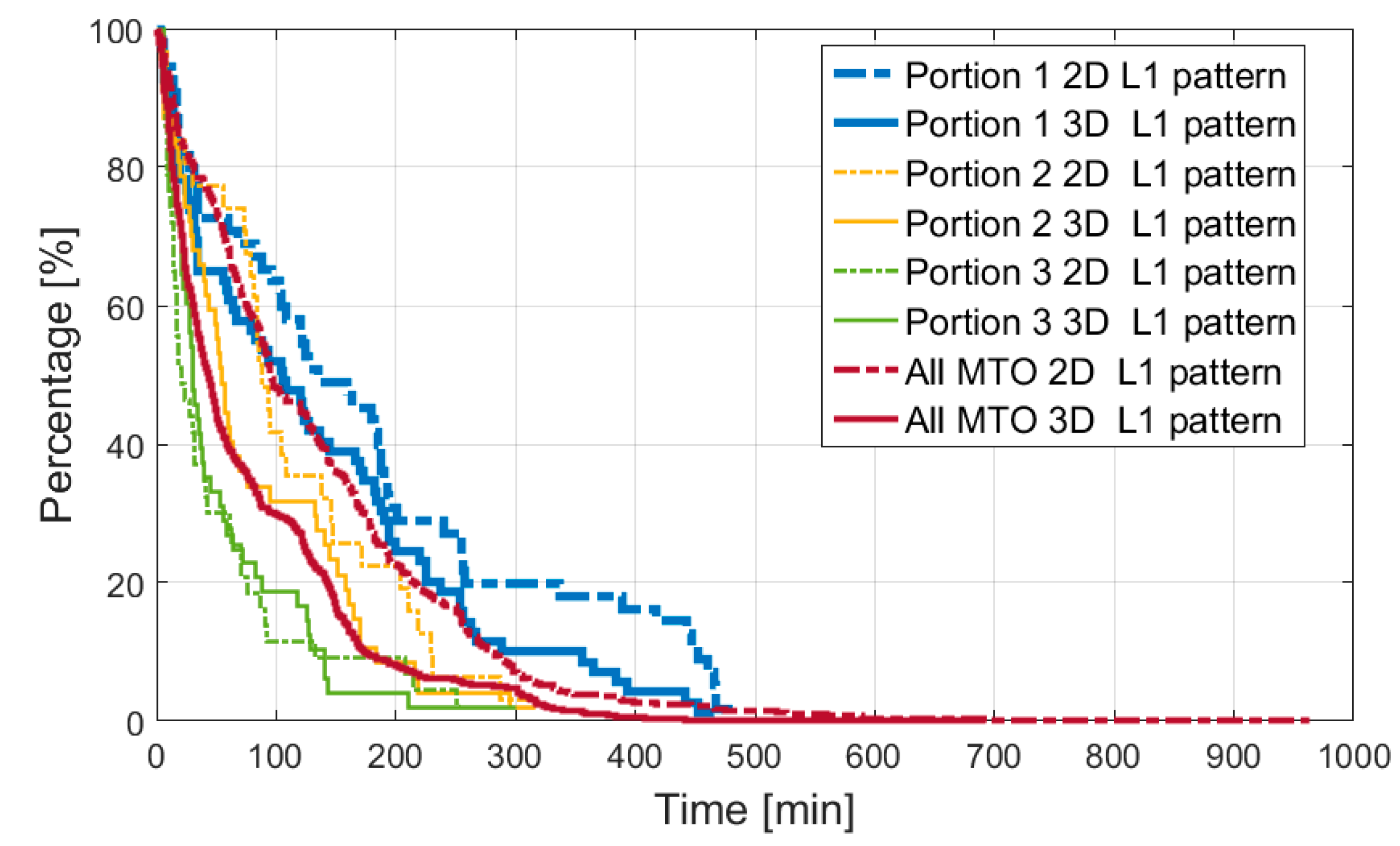
Figure 13.
Percentage of continuous time intervals, a point of each curve identifies a time interval duration T (on the x-axis) and the corresponding percentage (on the y-axis) of continuous time intervals equal or longer than T.
Figure 13.
Percentage of continuous time intervals, a point of each curve identifies a time interval duration T (on the x-axis) and the corresponding percentage (on the y-axis) of continuous time intervals equal or longer than T.
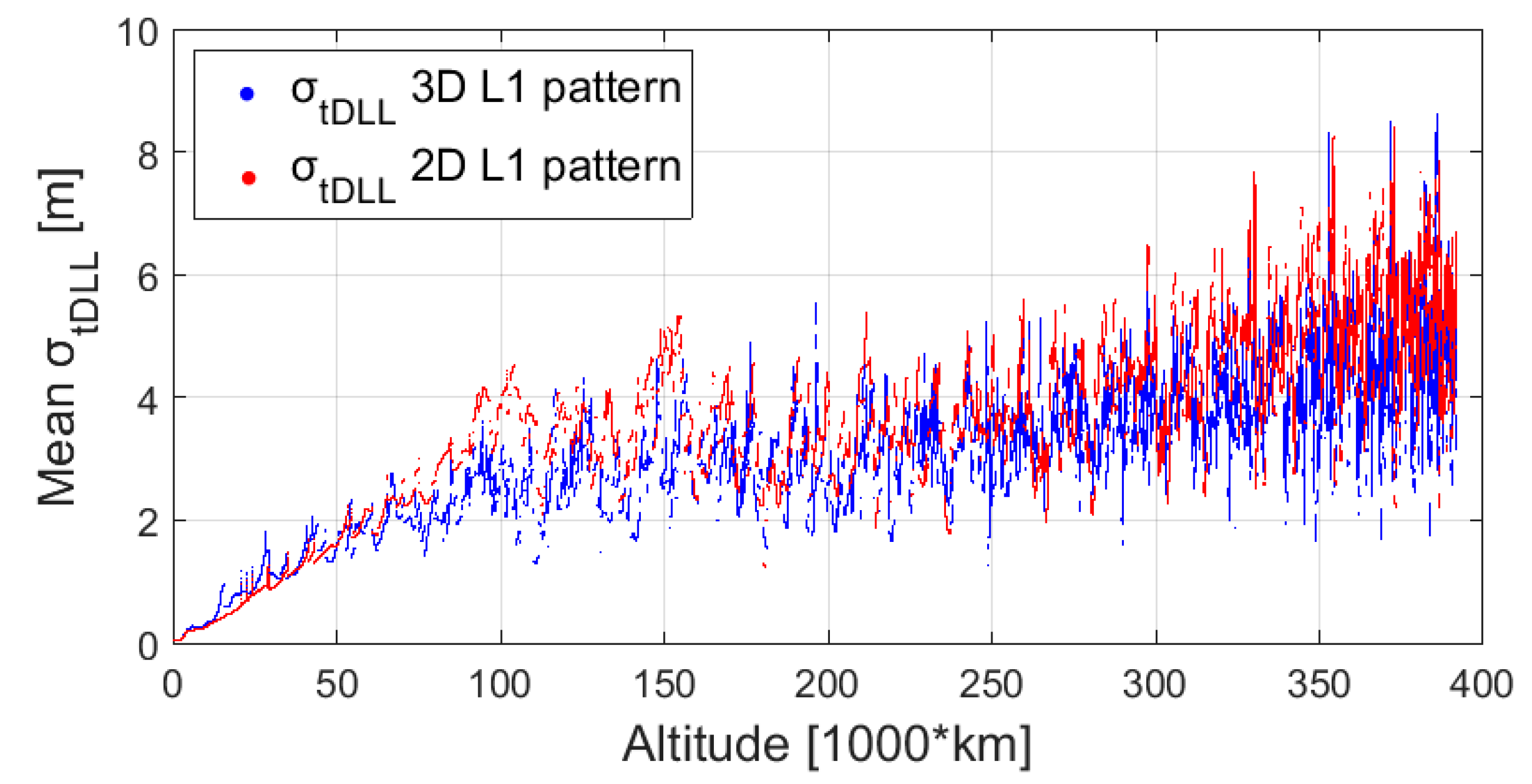
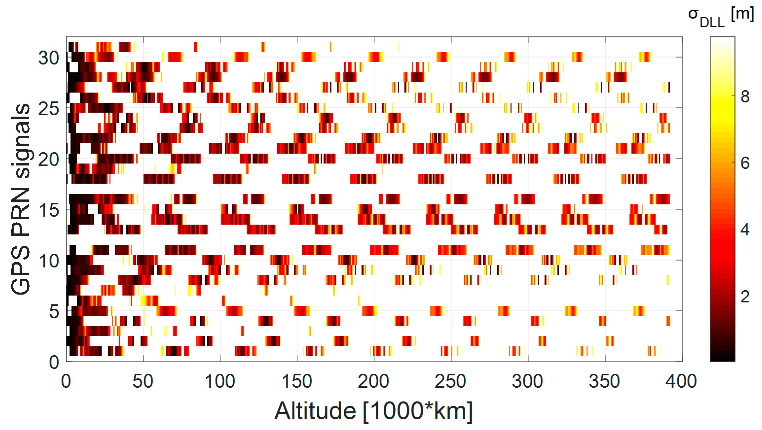
Figure 14.
Mean code tracking thermal noise range error, for the assumed MTO. The thermal noise range error is computed for each available pseudo random noise (PRN) and the mean is plotted.
Figure 14.
Mean code tracking thermal noise range error, for the assumed MTO. The thermal noise range error is computed for each available pseudo random noise (PRN) and the mean is plotted.
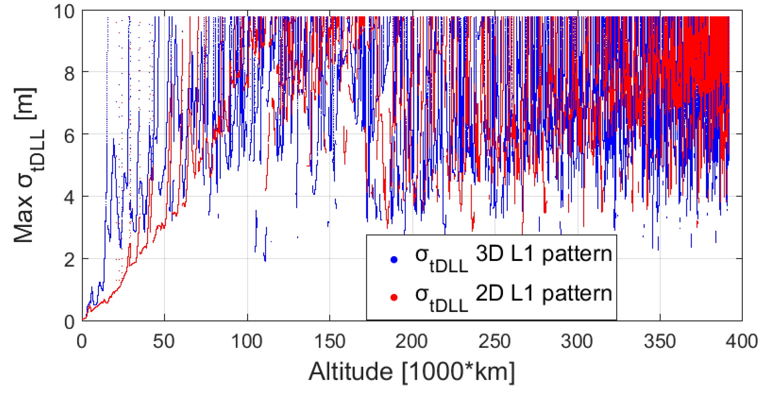
Figure 15.
Max code tracking thermal noise range error, for the assumed MTO. The thermal noise range error is computed for each available PRN and the max is plotted.
Figure 15.
Max code tracking thermal noise range error, for the assumed MTO. The thermal noise range error is computed for each available PRN and the max is plotted.
Figure 16.
, when assuming 3D transmitter patterns.
Figure 16.
, when assuming 3D transmitter patterns.
Figure 17.
Single-point least squares estimation error for the assumed MTO.
Figure 17.
Single-point least squares estimation error for the assumed MTO.
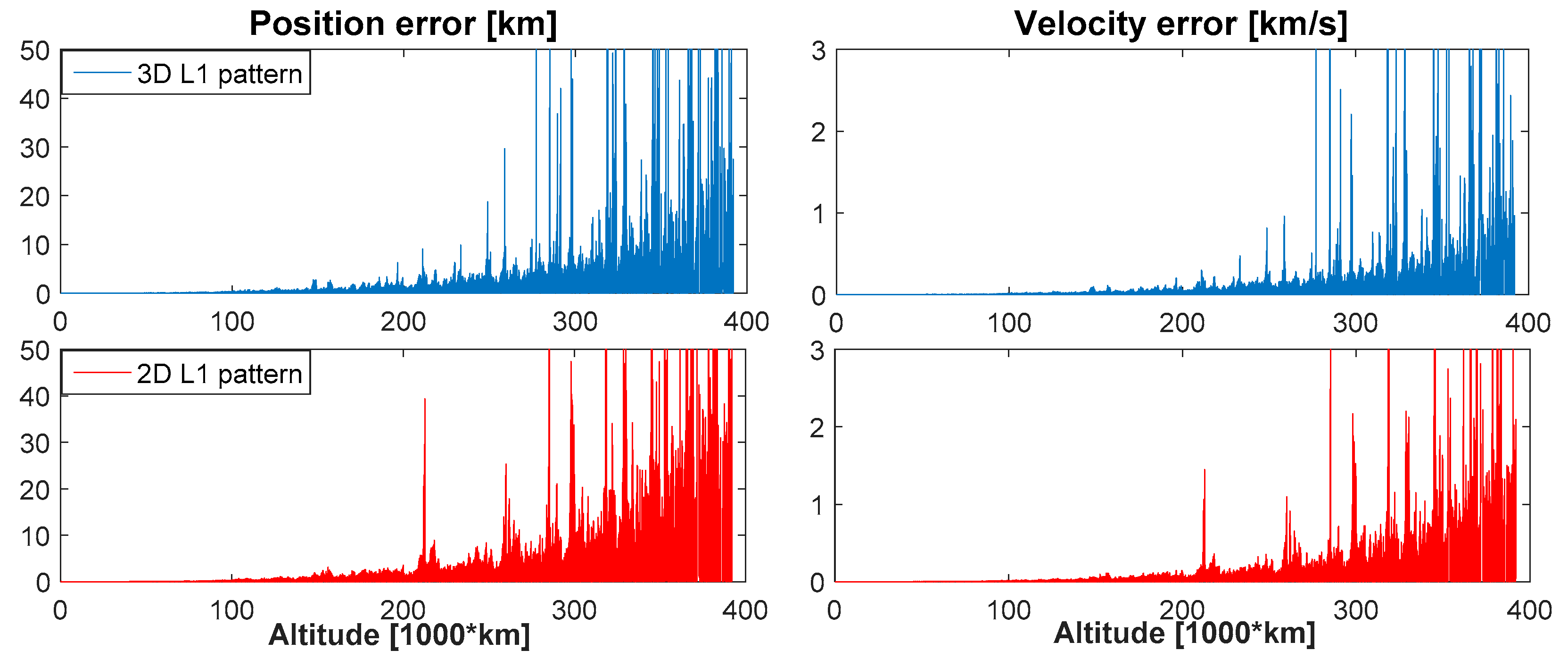
Figure 18.
Range-based orbital filter estimation error for the assumed MTO.
Figure 18.
Range-based orbital filter estimation error for the assumed MTO.
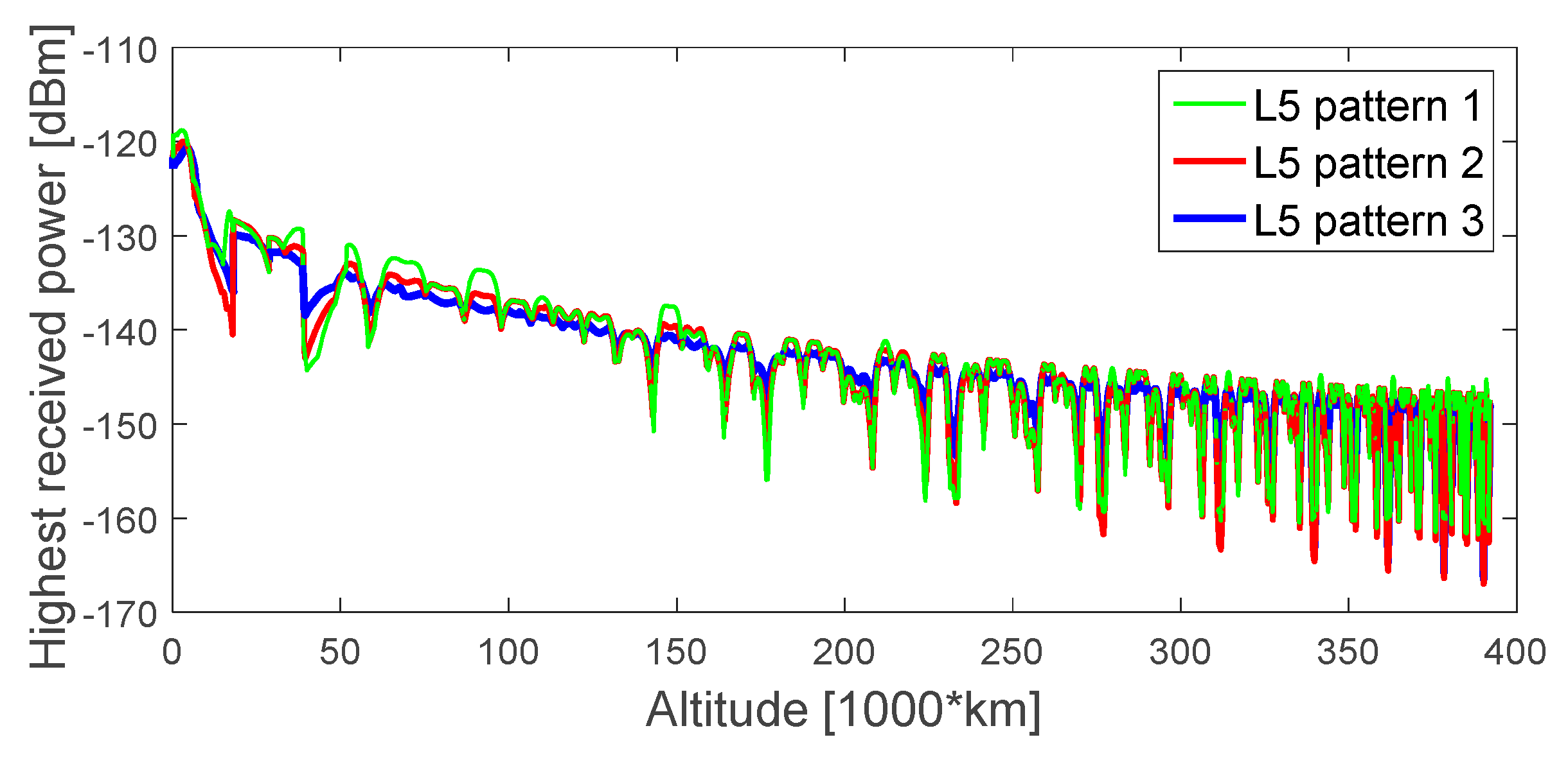
Figure 19.
Highest received power level of GPS L5 signals, during the considered MTO, for a 0 dBi receiver gain pattern.
Figure 19.
Highest received power level of GPS L5 signals, during the considered MTO, for a 0 dBi receiver gain pattern.
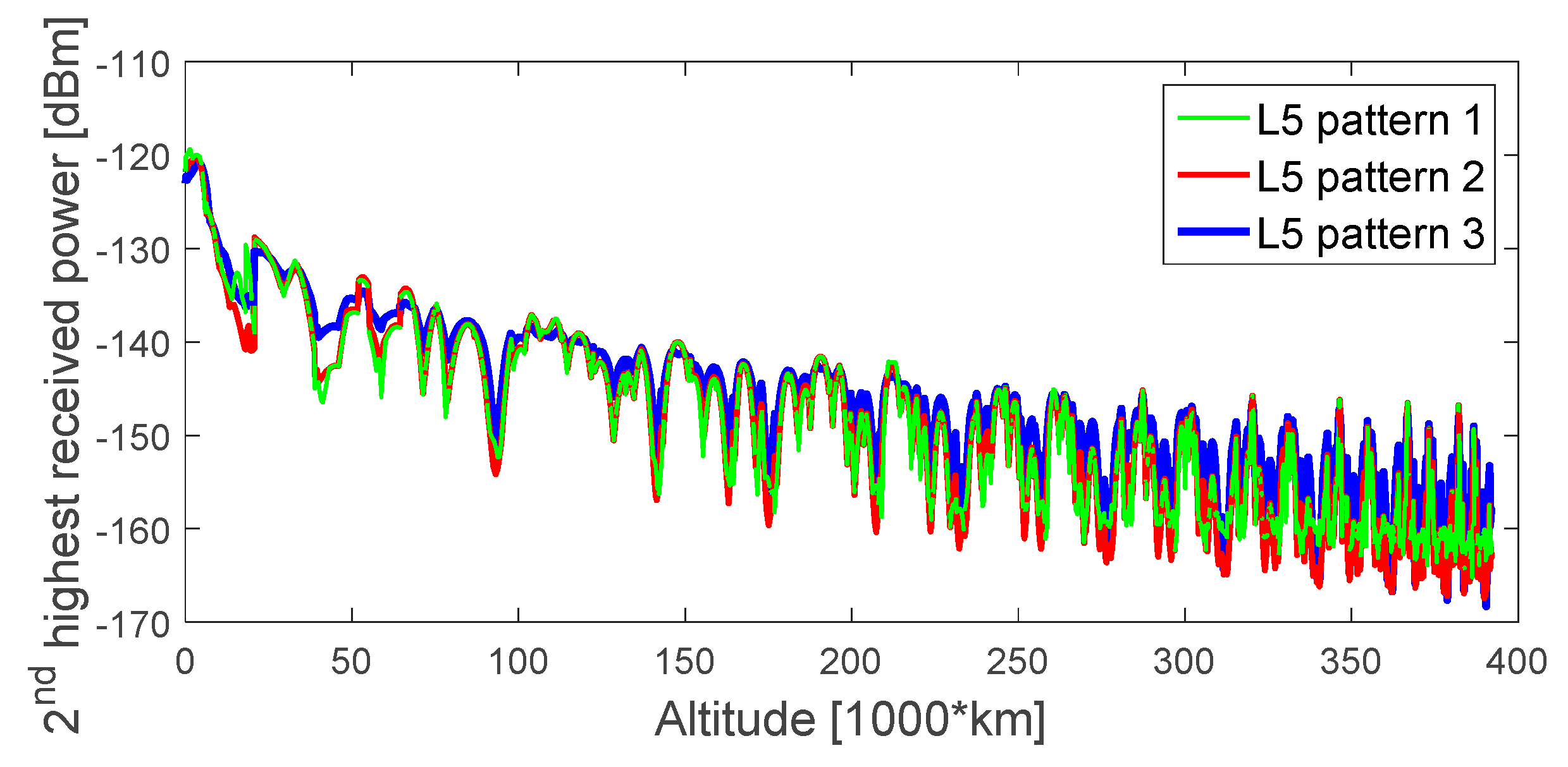
Figure 20.
Second-highest received power level of GPS L5 signals, during the considered MTO, for a 0 dBi receiver gain pattern.
Figure 20.
Second-highest received power level of GPS L5 signals, during the considered MTO, for a 0 dBi receiver gain pattern.
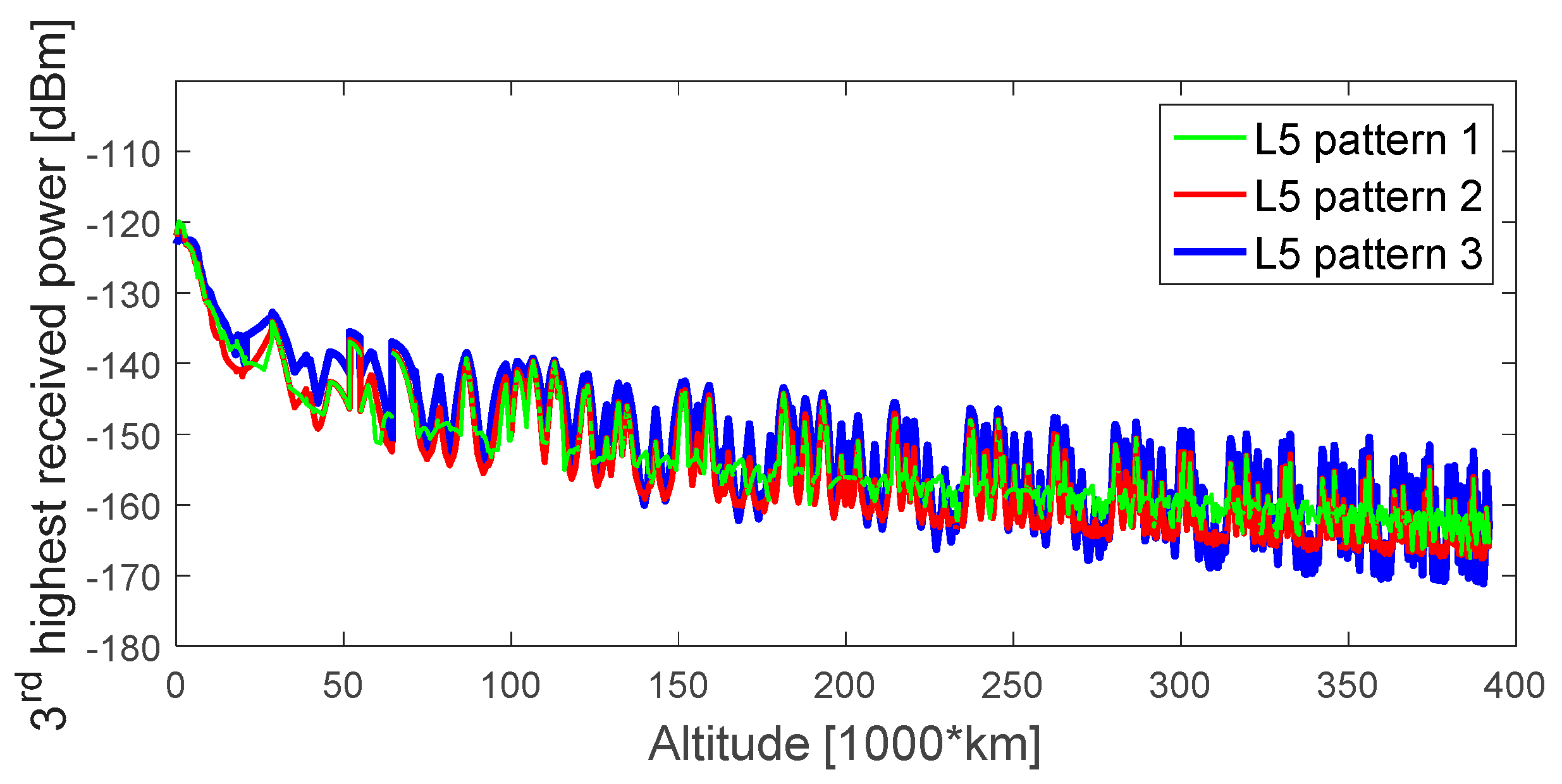
Figure 21.
Third-highest received power level of GPS L5 signals, during the considered MTO, for a 0 dBi receiver gain pattern.
Figure 21.
Third-highest received power level of GPS L5 signals, during the considered MTO, for a 0 dBi receiver gain pattern.
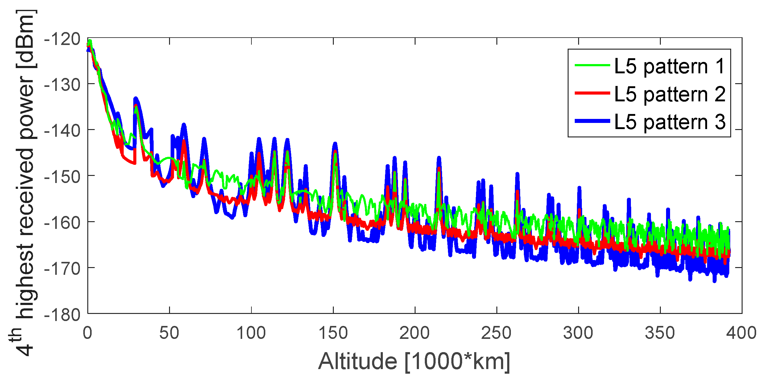
Figure 22.
Fourth-highest received power level of GPS L5 signals, during the considered MTO, for a 0 dBi receiver gain pattern.
Figure 22.
Fourth-highest received power level of GPS L5 signals, during the considered MTO, for a 0 dBi receiver gain pattern.
Figure 23.
Available GPS L5 signals, during the assumed MTO, for a 10 dBi receiver gain pattern.
Figure 23.
Available GPS L5 signals, during the assumed MTO, for a 10 dBi receiver gain pattern.
Figure 24.
Number of available observations during the assumed MTO.
Figure 24.
Number of available observations during the assumed MTO.
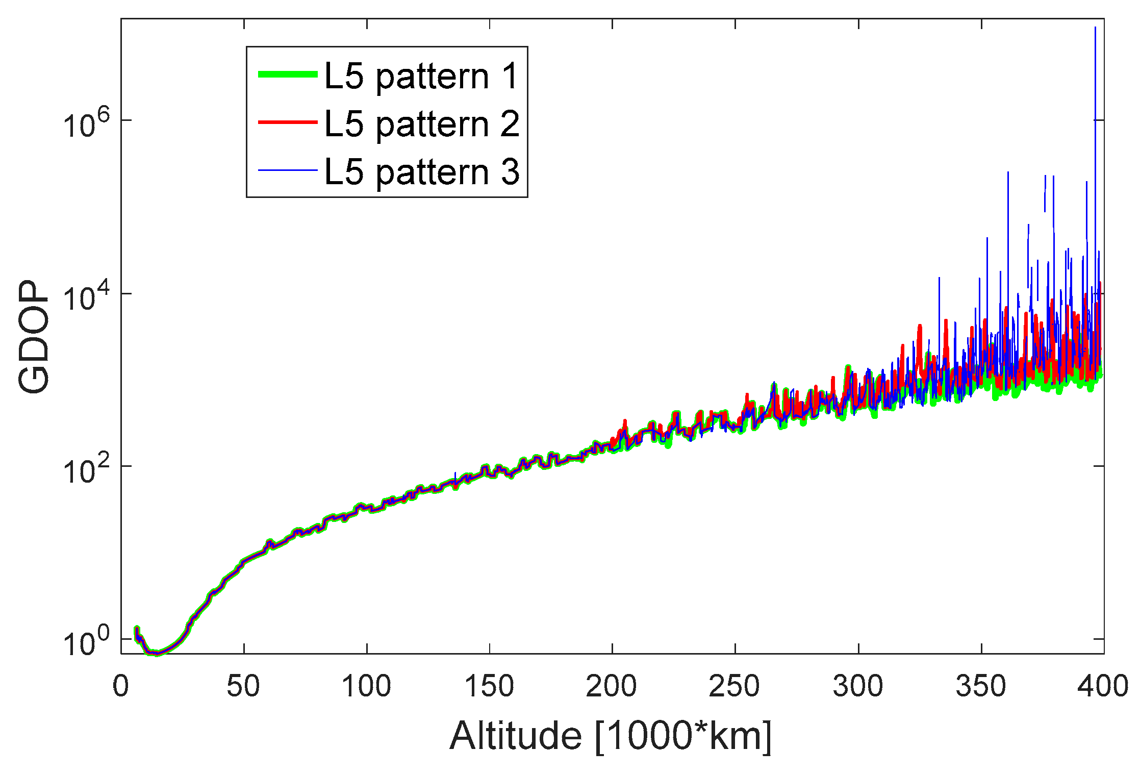
Figure 25.
GDOP in log scale during the assumed MTO.
Figure 25.
GDOP in log scale during the assumed MTO.
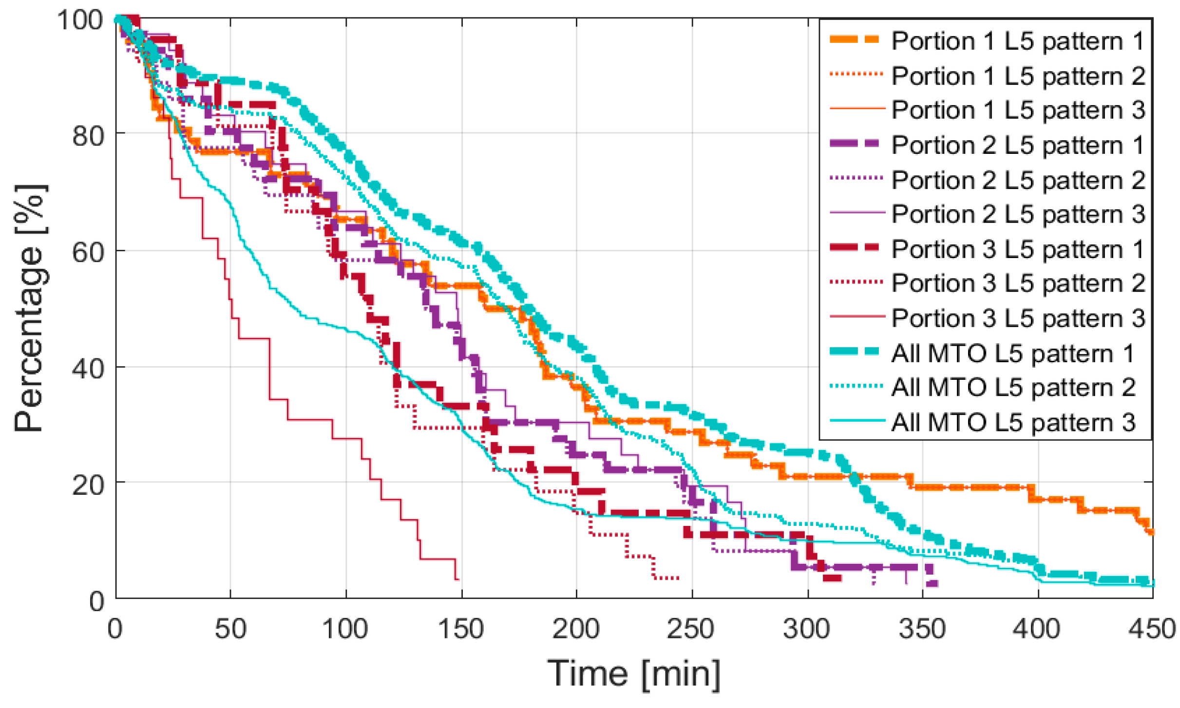
Figure 26.
Percentage of continuous time intervals, a point of each curve identifies a time interval duration T (on the x-axis) and the corresponding percentage (on the y-axis) of continuous time intervals equal or longer than T.
Figure 26.
Percentage of continuous time intervals, a point of each curve identifies a time interval duration T (on the x-axis) and the corresponding percentage (on the y-axis) of continuous time intervals equal or longer than T.
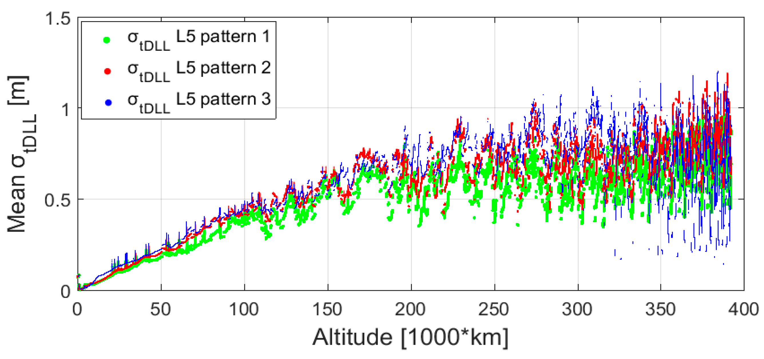
Figure 27.
Mean code tracking thermal noise range error for the assumed MTO. The thermal noise range error is computed for each available PRN and the mean is plotted.
Figure 27.
Mean code tracking thermal noise range error for the assumed MTO. The thermal noise range error is computed for each available PRN and the mean is plotted.
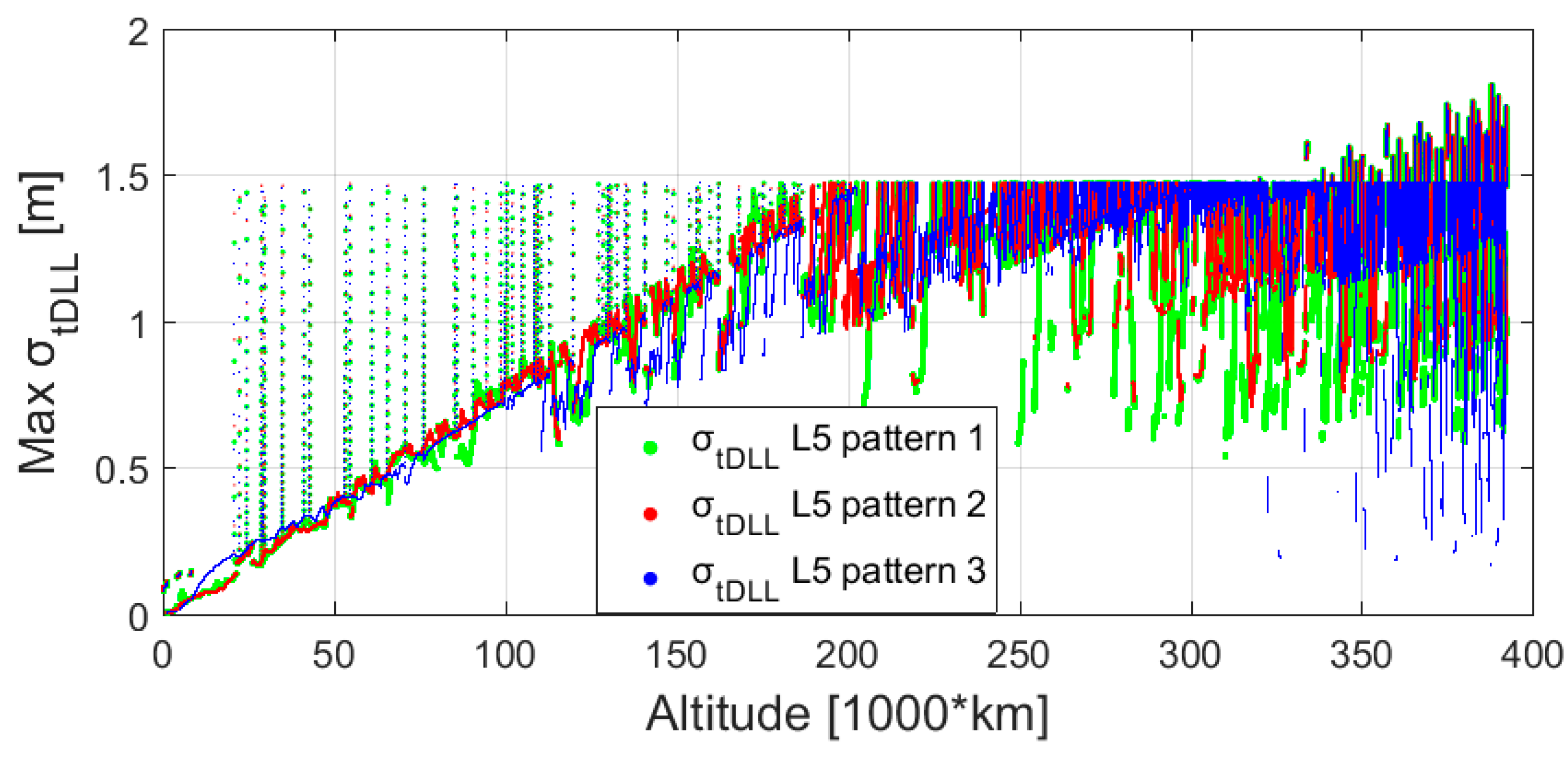
Figure 28.
Max code tracking thermal noise range error for the assumed MTO. The thermal noise range error is computed for each available PRN and the max is plotted.
Figure 28.
Max code tracking thermal noise range error for the assumed MTO. The thermal noise range error is computed for each available PRN and the max is plotted.
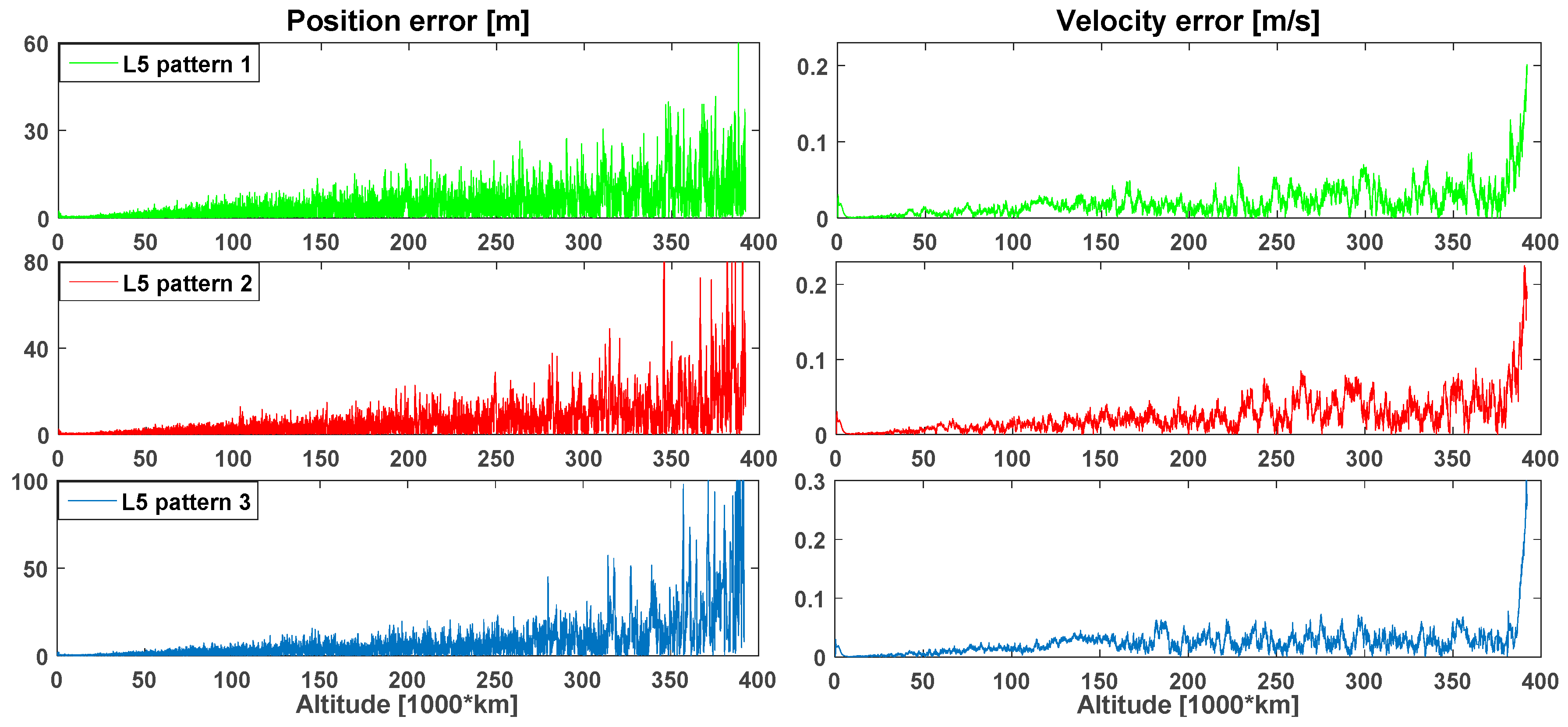
Figure 29.
Single-point least squares estimation error for the assumed MTO.
Figure 29.
Single-point least squares estimation error for the assumed MTO.
Figure 30.
Range-based orbital filter estimation error for the assumed MTO.
Figure 30.
Range-based orbital filter estimation error for the assumed MTO.
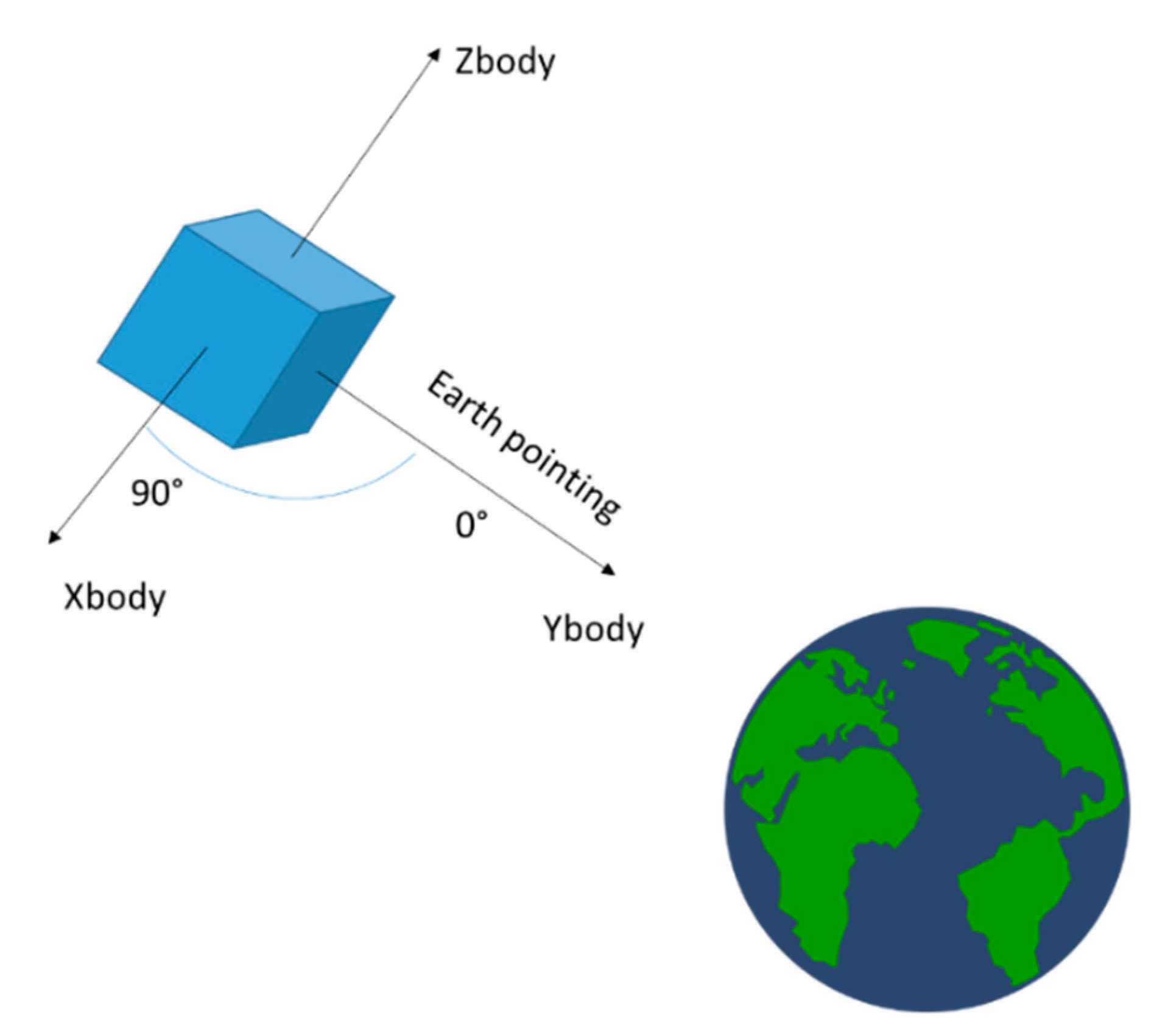
Figure 31.
Earth-pointing attitude configuration assumed for the receiver.
Figure 31.
Earth-pointing attitude configuration assumed for the receiver.
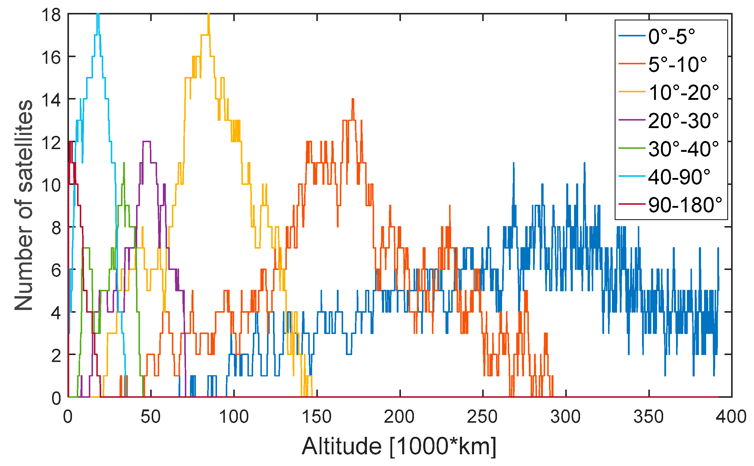
Figure 32.
Number of available global navigation satellite system (GNSS) observations for each receiver antenna elevation for each altitude of the whole considered MTO.
Figure 32.
Number of available global navigation satellite system (GNSS) observations for each receiver antenna elevation for each altitude of the whole considered MTO.
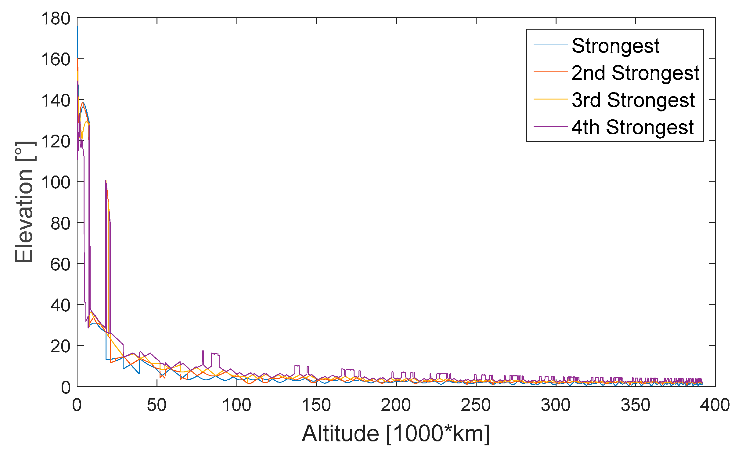
Figure 33.
Elevation values at which the four strongest signals are available at the receiver’s antenna.
Figure 33.
Elevation values at which the four strongest signals are available at the receiver’s antenna.
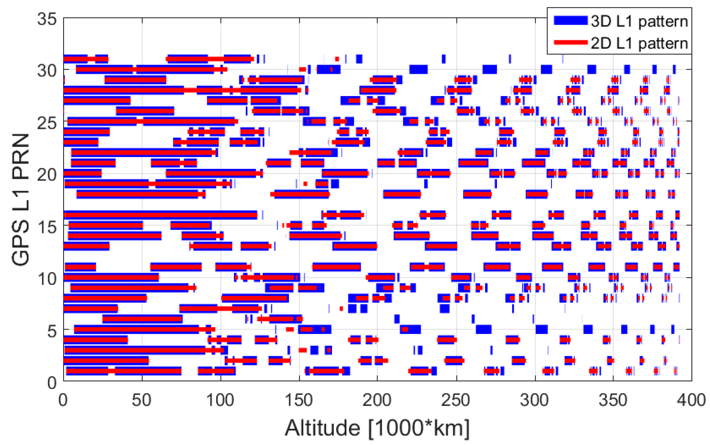
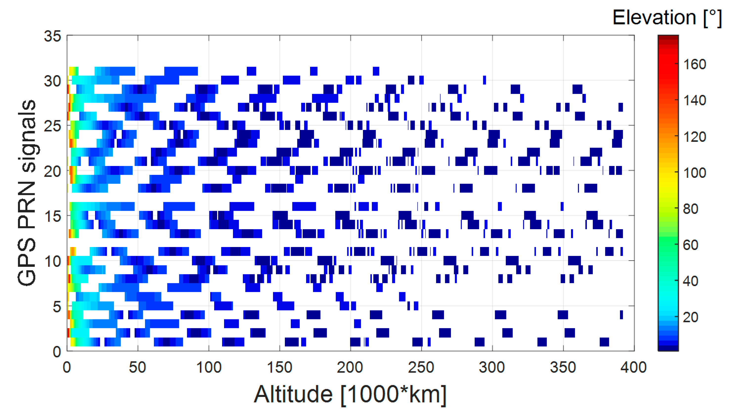
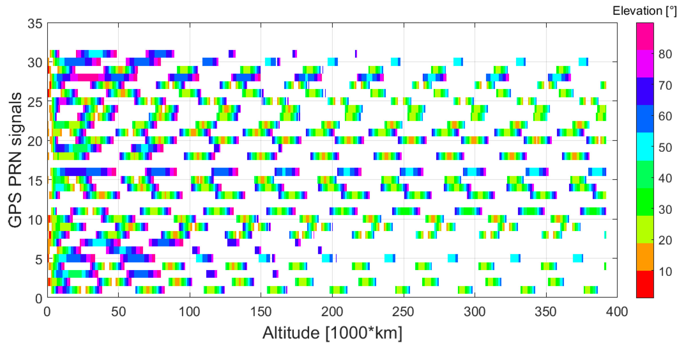
Figure 34.
PRNs available for each receiver’s antenna elevation for each altitude of the whole considered MTO.
Figure 34.
PRNs available for each receiver’s antenna elevation for each altitude of the whole considered MTO.
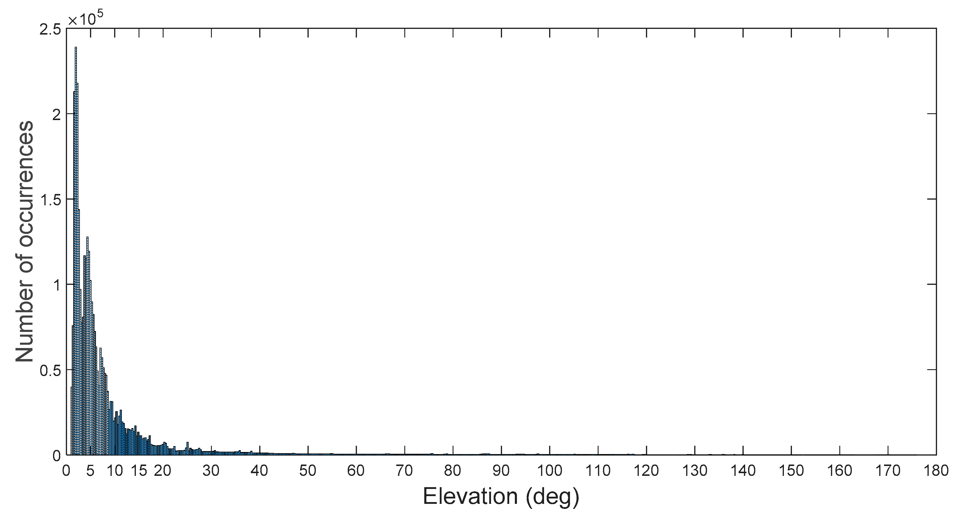
Figure 35.
Histogram of the available observations for each receiver’s antenna elevation during the whole considered MTO.
Figure 35.
Histogram of the available observations for each receiver’s antenna elevation during the whole considered MTO.
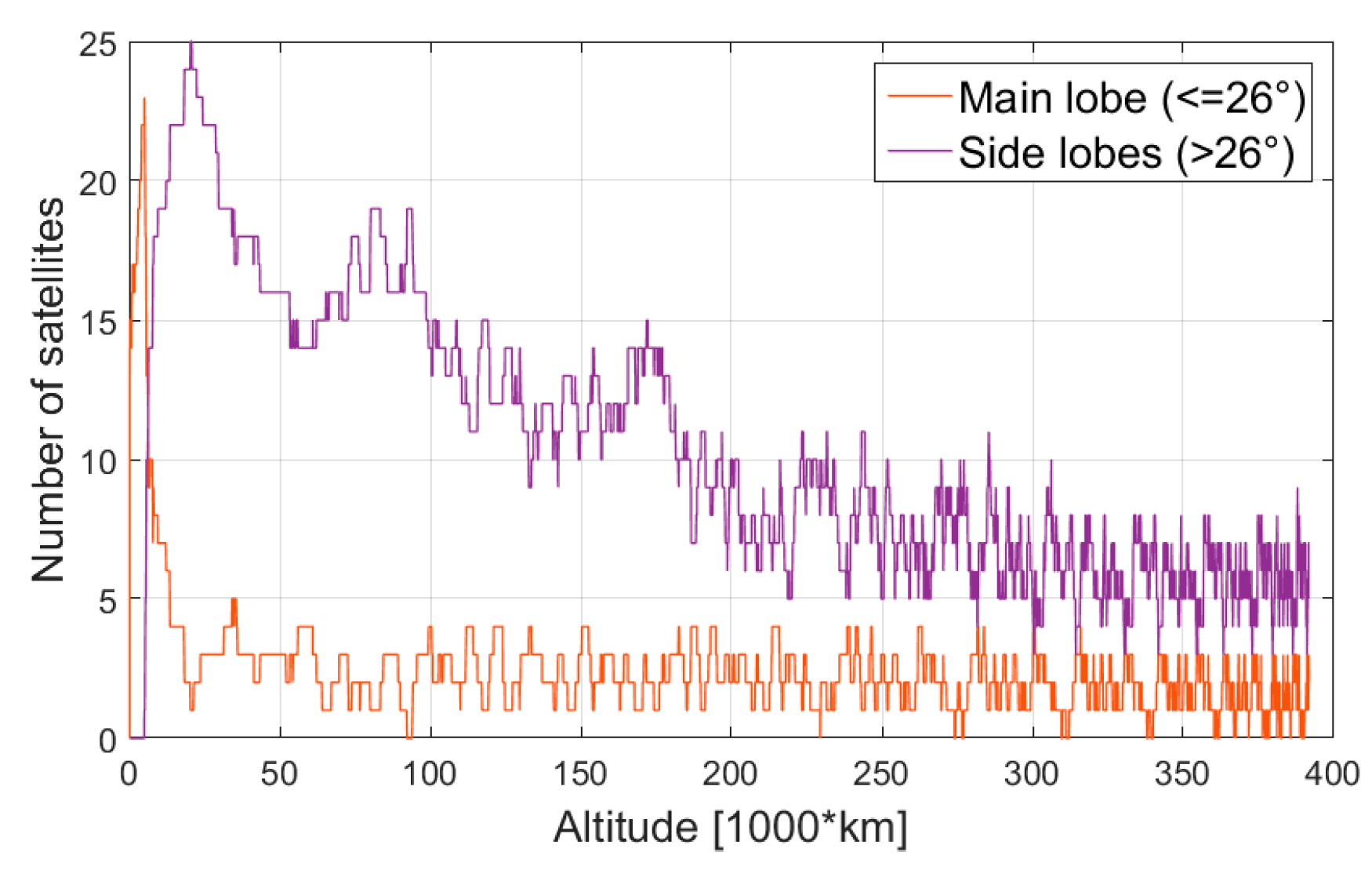
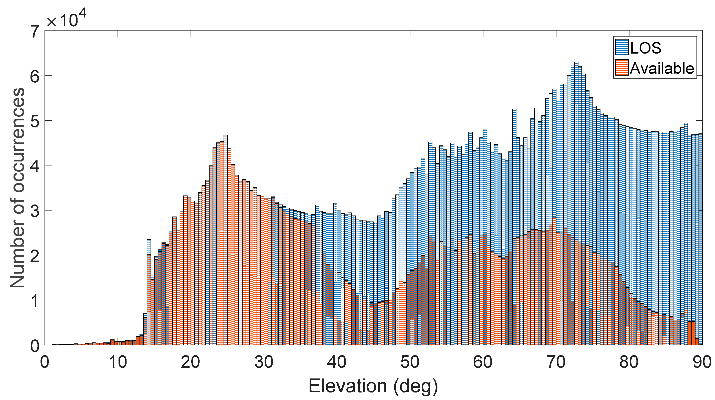
Figure 36.
Histogram of the visible satellites (in the line of sight (LOS)) and of the available satellites (the ones from which the signal transmitted is strong enough to be acquired and tracked be the SANAG receiver) for each transmitter’s antenna elevation during the whole considered MTO.
Figure 36.
Histogram of the visible satellites (in the line of sight (LOS)) and of the available satellites (the ones from which the signal transmitted is strong enough to be acquired and tracked be the SANAG receiver) for each transmitter’s antenna elevation during the whole considered MTO.
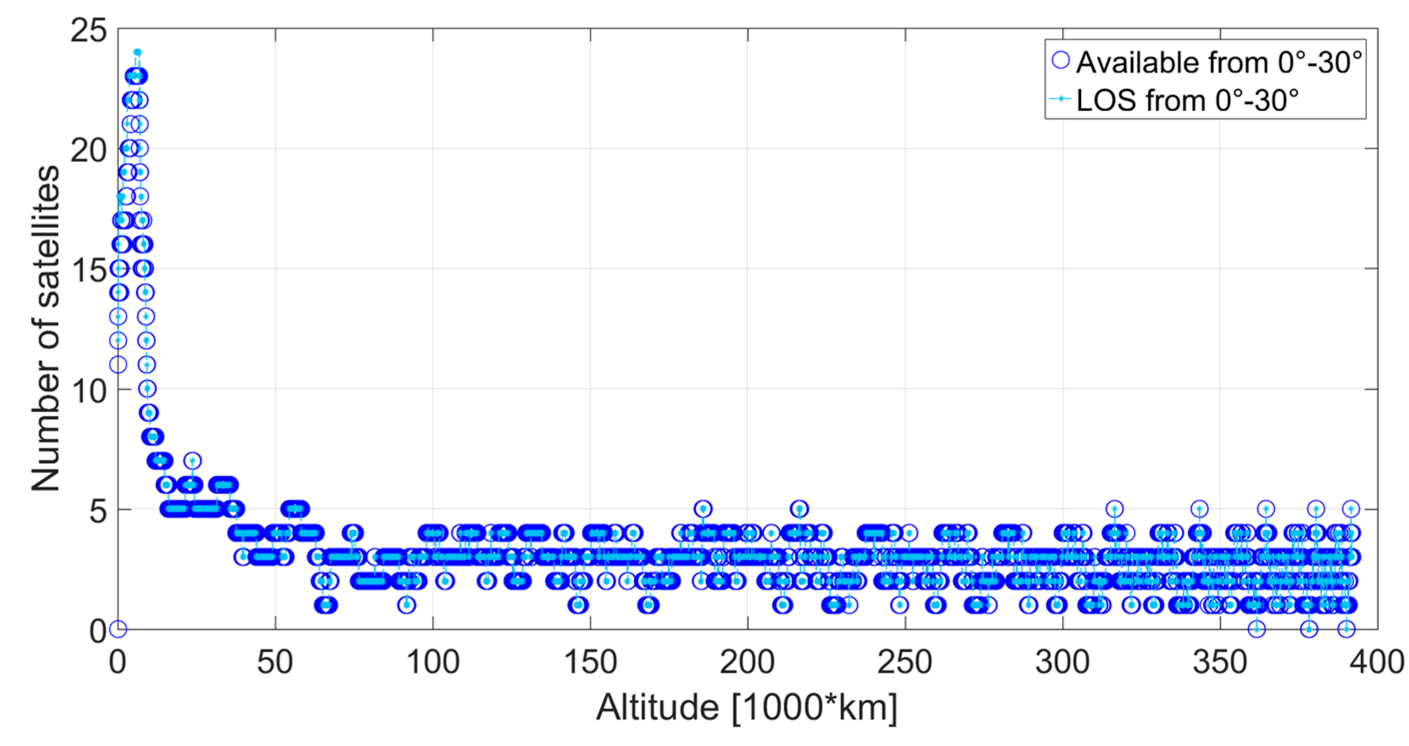
Figure 37.
Visible satellites (in the line of sight (LOS)) and available satellites at the receiver’s position, for which the corresponding signal is transmitted at an angle between 0° and 30° from the transmitter’s boresight.
Figure 37.
Visible satellites (in the line of sight (LOS)) and available satellites at the receiver’s position, for which the corresponding signal is transmitted at an angle between 0° and 30° from the transmitter’s boresight.
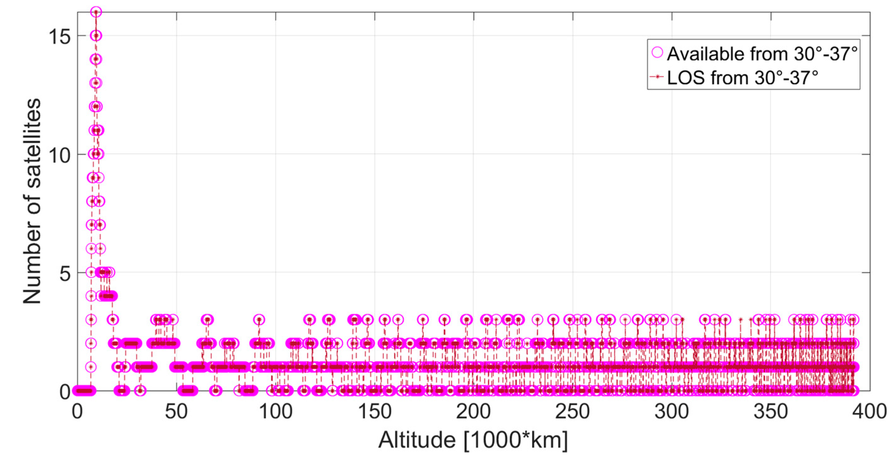
Figure 38.
Visible satellites (in the line of sight (LOS)) and available satellites at the receiver’s position, for which the corresponding signal is transmitted at an angle between 30° and 37° from the transmitter’s boresight.
Figure 38.
Visible satellites (in the line of sight (LOS)) and available satellites at the receiver’s position, for which the corresponding signal is transmitted at an angle between 30° and 37° from the transmitter’s boresight.
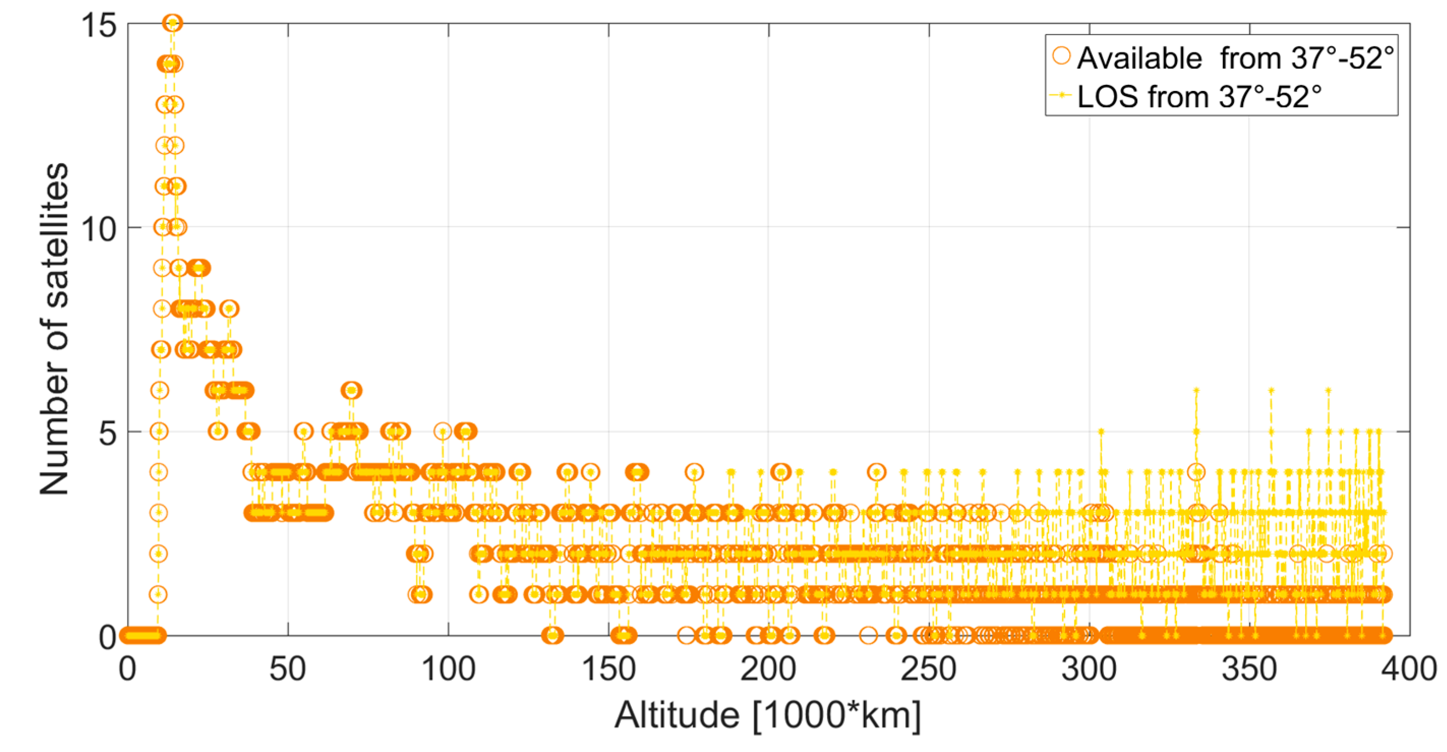
Figure 39.
Visible satellites (in the line of sight (LOS)) and available satellites at the receiver’s position, for which the corresponding signal is transmitted at an angle between 37° and 52° from the transmitter’s boresight.
Figure 39.
Visible satellites (in the line of sight (LOS)) and available satellites at the receiver’s position, for which the corresponding signal is transmitted at an angle between 37° and 52° from the transmitter’s boresight.
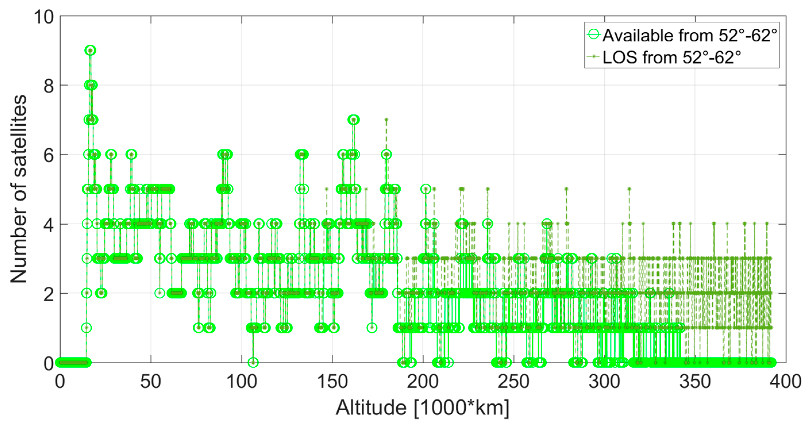
Figure 40.
Visible satellites (in the line of sight (LOS)) and available satellites at the receiver’s position, for which the corresponding signal is transmitted at an angle between 52° and 62° from the transmitter’s boresight.
Figure 40.
Visible satellites (in the line of sight (LOS)) and available satellites at the receiver’s position, for which the corresponding signal is transmitted at an angle between 52° and 62° from the transmitter’s boresight.
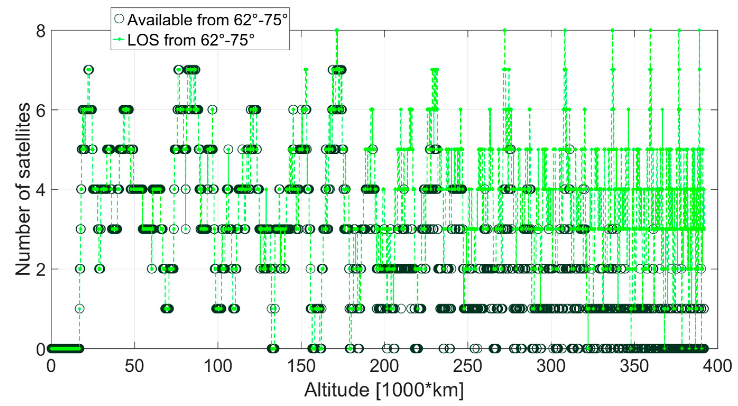
Figure 41.
Visible satellites (in the line of sight (LOS)) and available satellites at the receiver’s position, for which the corresponding signal is transmitted at an angle between 62° and 75° from the transmitter’s boresight.
Figure 41.
Visible satellites (in the line of sight (LOS)) and available satellites at the receiver’s position, for which the corresponding signal is transmitted at an angle between 62° and 75° from the transmitter’s boresight.
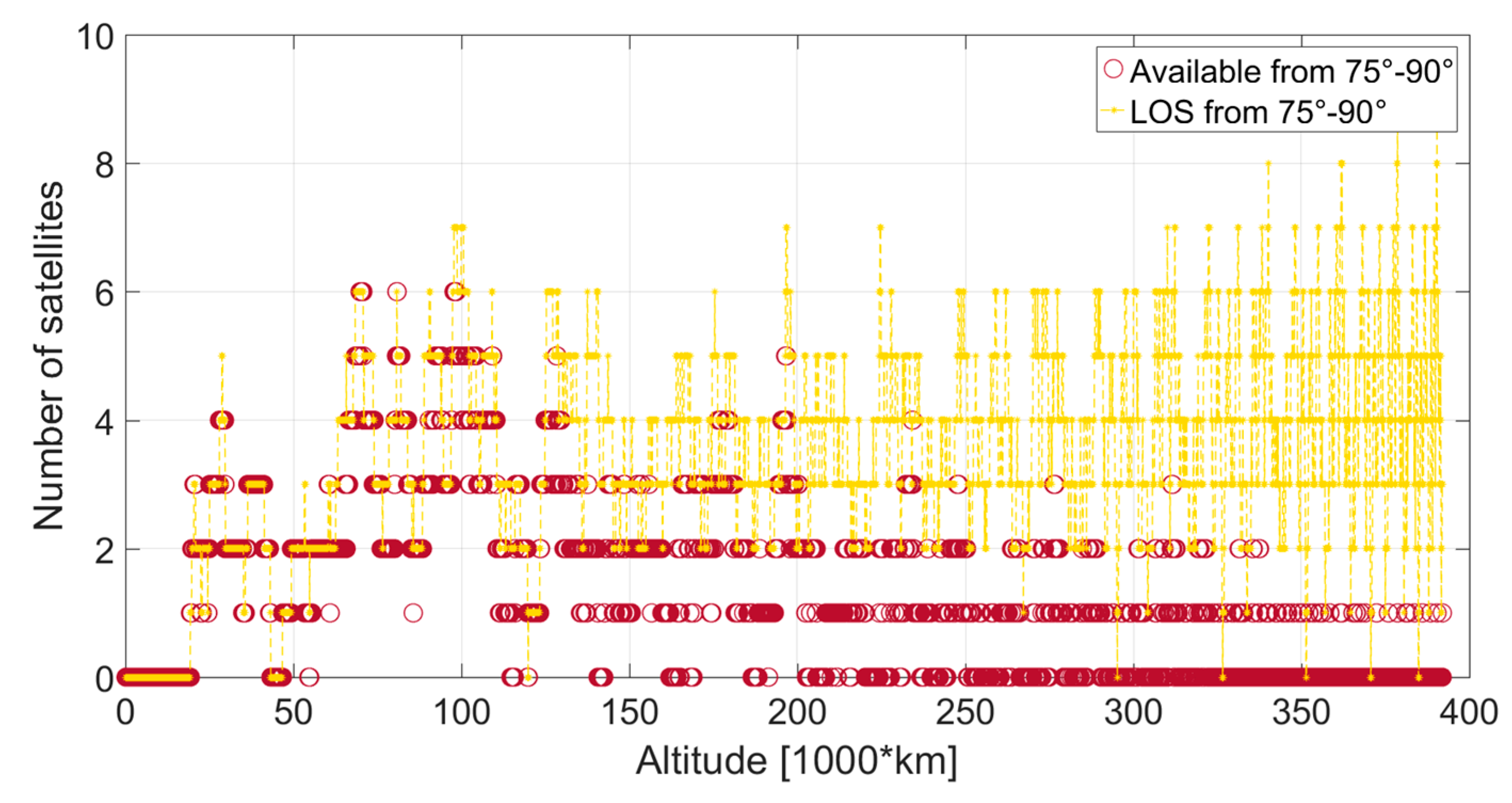
Figure 42.
Visible satellites (in the line of sight (LOS)) and available satellites at the receiver’s position, for which the corresponding signal is transmitted at an angle between 75° and 90° from the transmitter’s boresight.
Figure 42.
Visible satellites (in the line of sight (LOS)) and available satellites at the receiver’s position, for which the corresponding signal is transmitted at an angle between 75° and 90° from the transmitter’s boresight.
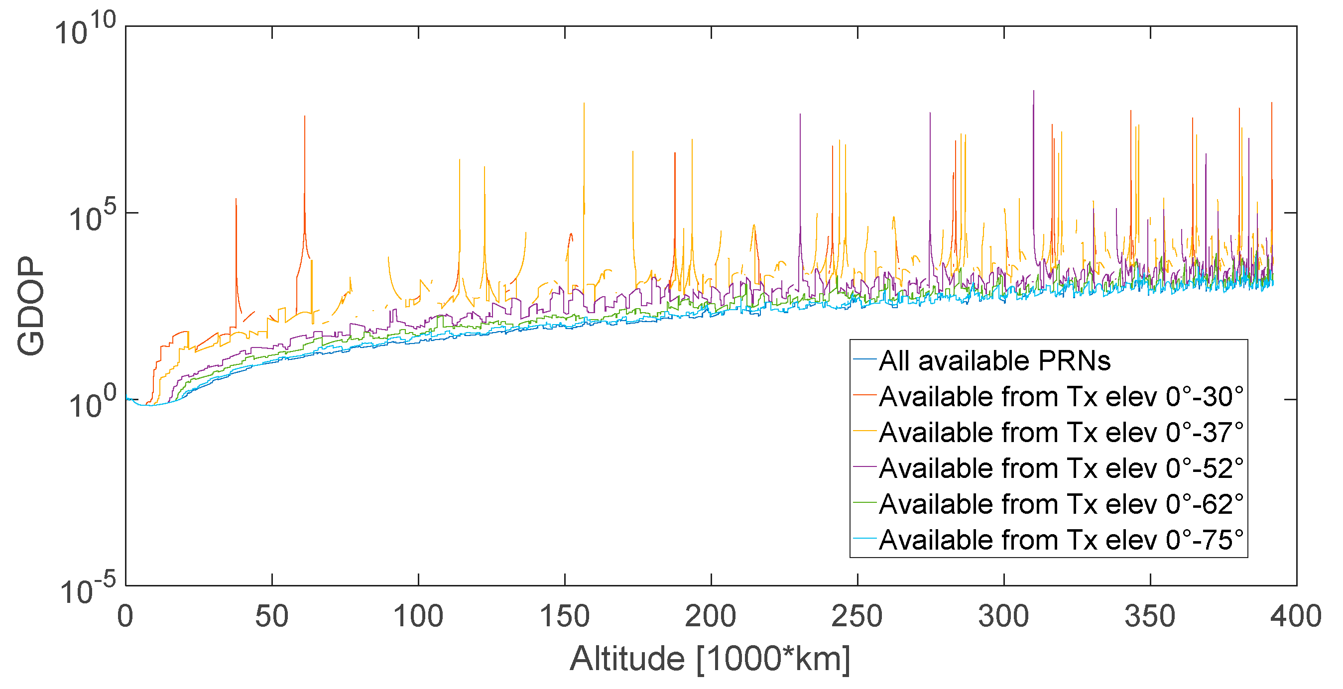
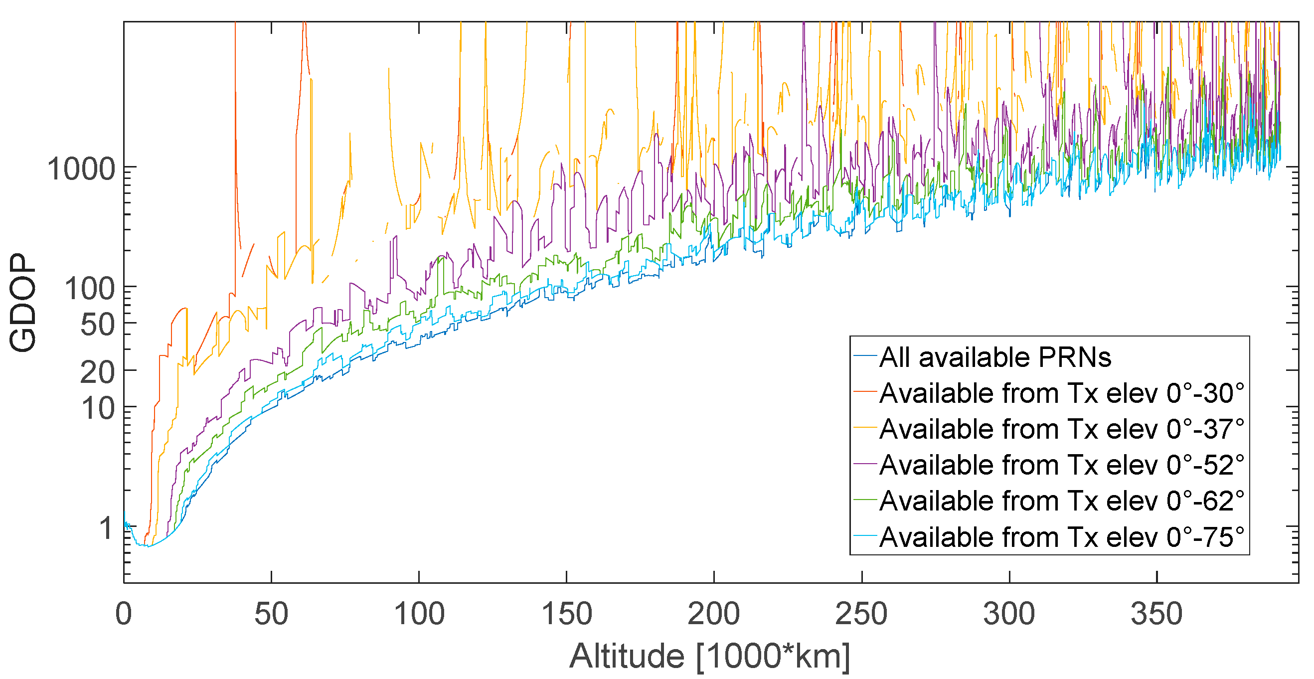
Figure 43.
GDOP computed when using all the available signals (each identified by a PRN) and only the ones transmitted at angle between 0° and 30°, 0° and 37°, 0° and 52°, 0° and 62°, 0° and 75°, and 0° and 90°.
Figure 43.
GDOP computed when using all the available signals (each identified by a PRN) and only the ones transmitted at angle between 0° and 30°, 0° and 37°, 0° and 52°, 0° and 62°, 0° and 75°, and 0° and 90°.
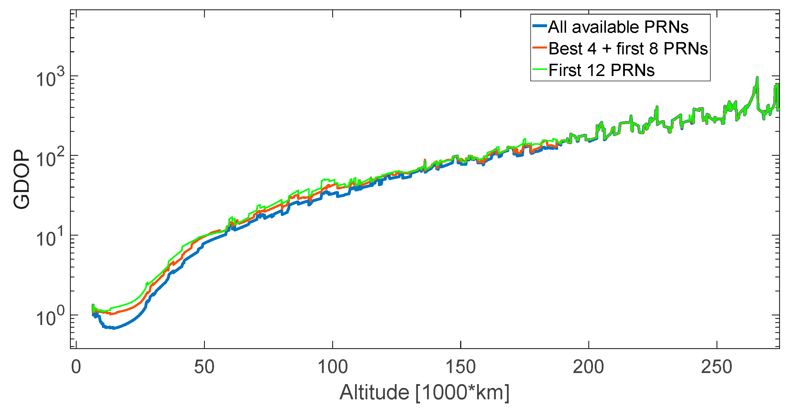
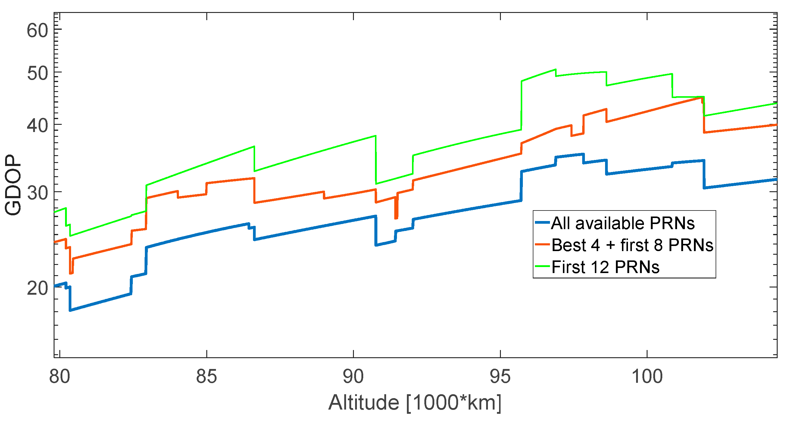
Figure 45.
GDOP in three different cases: when all the available signals are processed (in blue), when only the first 12 signals available are processed (in green, i.e., chronologically the first 12 available from 1 to 29), when the four signals that provide the lowest GDOP are included in the 12 processed (in brown).
Figure 46.
Zoomed-in version of
Figure 45 between 80,000 km and 105,000 km.
Figure 46.
Zoomed-in version of
Figure 45 between 80,000 km and 105,000 km.
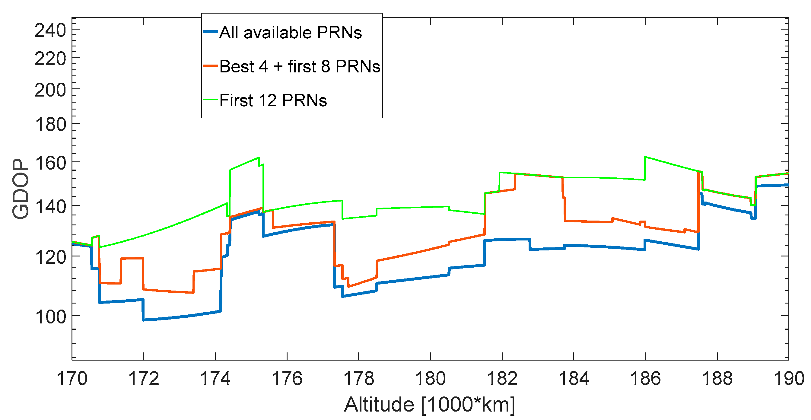
Figure 47.
Zoomed-in version of
Figure 45 between 170,000 km and 190,000 km.
Figure 47.
Zoomed-in version of
Figure 45 between 170,000 km and 190,000 km.
Table 1.
Observations and assumptions.
Table 1.
Observations and assumptions.
| Pseudorange | |
| : i-th satellite coordinates at time of transmission |
| : the receiver coordinates at time of reception |
| : receiver clock offset at signal reception time | initial value: 10 km |
| : transmitter clock offset at signal transmission time |
| : atmospheric delay (m) | 7 m (when the receiver is orbiting below the ionosphere upper bound) |
| : multipath delay (m) | 0.2 m |
| : signal-in-space ranging error (SISRE) (m) | 0.5 m |
| : receiver noise (m) | |
| Pseudorange rate | |
| : i-th satellite’s velocity vector |
| : receiver’s velocity vector |
| : the line of sight (LOS) unit vector from the receiver to the i-th GNSS satellite |
| : receiver clock drift | initial value: 100 m/s |
| : Doppler tracking jitter (m/s) |
Table 2.
Definition of representative portions.
Table 2.
Definition of representative portions.
| Portion Definition | Portion 1 | Portion 2 | Portion 3 |
|---|
| Time interval (min) | 5–505 | 1446–1946 | 5921–6421 |
| Distance from Earth interval (km) | 6530–100,506 | 200,000–237,891 | 391,219–398,317 |
Table 3.
Statistics for the number of available observations.
Table 3.
Statistics for the number of available observations.
| Portion | L1 Antenna Pattern 3D | L1 Antenna Pattern 2D |
|---|
| 1 | 2 | 3 | All MTO | 1 | 2 | 3 | All MTO |
|---|
| Average availability (%) | 60.21 | 25.19 | 16.58 | 24.61 | 62.63 | 22.49 | 14.06 | 24.01 |
| Mean | 18.67 | 7.81 | 5.14 | 7.63 | 19.42 | 6.97 | 4.36 | 7.44 |
| Max | 26 | 11 | 9 | 26 | 26 | 9 | 7 | 26 |
| Min | 11 | 5 | 1 | 1 | 11 | 4 | 2 | 1 |
Table 4.
Statistics of the single-point least squares estimation error.
Table 4.
Statistics of the single-point least squares estimation error.
| Portion | L1 Antenna Pattern 3D | L1 Antenna Pattern 2D |
|---|
| 1 | 2 | 3 | All MTO | 1 | 2 | 3 | All MTO |
|---|
| Position error (m) | Mean | 22.6 | 602.0 | 4976.2 | 135,948.0 | 23.5 | 978.2 | 10,973.4 | 4290.7 |
| Std | 27.9 | 594.6 | 5266.6 | 6,474,173.1 | 31.1 | 1490.1 | 162,226.0 | 41,018.5 |
| Max | 314.4 | 9080.8 | 124,313.9 | 381,775,899.5 | 288.6 | 39,294.8 | 19,249,062.5 | 19,249,062.5 |
| Velocity error (m/s) | Mean | 0.9 | 24.5 | 197 | 2620 | 0.9 | 38.7 | 1066 | 206 |
| Std | 1.1 | 24.1 | 207 | 206,914 | 1.2 | 60.2 | 56,428 | 13,801 |
| Max | 11.0 | 300.0 | 4027 | 69,692,351 | 11.7 | 1445.4 | 7,249,068 | 7,249,068 |
Table 5.
Statistics of the range-based orbital filter estimation error.
Table 5.
Statistics of the range-based orbital filter estimation error.
| Portion | L1 Antenna Pattern 3D | L1 Antenna Pattern 2D |
|---|
| 1 | 2 | 3 | All MTO | 1 | 2 | 3 | All MTO |
|---|
| Position error (m) | Mean | 2.93 | 16.57 | 88.45 | 36.12 | 3.16 | 22.18 | 89.86 | 45.07 |
| Std | 2.51 | 11.26 | 60.04 | 35.09 | 2.86 | 15.70 | 59.82 | 44.31 |
| Max | 30.42 | 72.42 | 232.03 | 232.03 | 25.33 | 98.61 | 302.79 | 302.79 |
| Velocity error (m/s) | Mean | 0.008 | 0.017 | 0.097 | 0.027 | 0.006 | 0.015 | 0.108 | 0.033 |
| Std | 0.005 | 0.007 | 0.030 | 0.025 | 0.004 | 0.007 | 0.035 | 0.029 |
| Max | 0.021 | 0.041 | 0.205 | 0.205 | 0.018 | 0.039 | 0.208 | 0.208 |
Table 6.
Statistics for the number of available observations.
Table 6.
Statistics for the number of available observations.
| Portion | L5 Antenna Pattern 1 | L5 Antenna Pattern 2 | L5 Antenna Pattern 3 |
|---|
| 1 | 2 | 3 | MTO | 1 | 2 | 3 | MTO | 1 | 2 | 3 | MTO |
|---|
| Average availability (%) | 63.42 | 33.70 | 22.99 | 32.17 | 63.42 | 32.00 | 20.05 | 30.16 | 63.35 | 35.03 | 12.06 | 27.65 |
| Mean | 19.66 | 10.45 | 7.13 | 9.97 | 19.66 | 9.92 | 6.21 | 9.35 | 19.64 | 10.86 | 3.74 | 8.57 |
| Max | 26 | 13 | 10 | 26 | 26 | 12 | 9 | 26 | 26 | 13 | 7 | 26 |
| Min | 11 | 8 | 5 | 5 | 11 | 8 | 4 | 4 | 11 | 8 | 1 | 1 |
| ≥4 sats (%) | 100 | 100 | 100 | 100 | 100 | 100 | 100 | 100 | 100 | 100 | 62.52 | 88.15 |
Table 7.
Statistics of the single-point least squares estimation error.
Table 7.
Statistics of the single-point least squares estimation error.
| Portion | L5 Antenna Pattern 1 | L5 Antenna Pattern 2 | L5 Antenna Pattern 3 |
|---|
| 1 | 2 | 3 | All MTO | 1 | 2 | 3 | All MTO | 1 | 2 | 3 | All MTO |
|---|
| Position error (m) | Mean | 5.6 | 123.9 | 717 | 358 | 5.8 | 144.1 | 1339 | 591 | 5.6 | 130.8 | 5874 | 1026 |
| Std | 6.5 | 102.9 | 627 | 462 | 6.7 | 115.7 | 1504 | 930 | 6.5 | 103.9 | 26,843 | 7761 |
| Max | 71 | 906 | 6052 | 6615 | 58 | 1419 | 22,163 | 22,163 | 59 | 826 | 2,123,291 |
| Velocity error (m/s) | Mean | 0.84 | 39.0 | 204 | 103 | 1.02 | 49.1 | 493 | 204 | 0.89 | 44.0 | 1532 | 271 |
| Std | 1.17 | 34.2 | 176 | 131 | 1.39 | 39.9 | 603 | 334 | 1.19 | 36.4 | 37,712 | 7466 |
| Max | 13.9 | 323.7 | 2192 | 2192 | 12.9 | 327.7 | 9775 | 9775 | 14.1 | 341.9 | 4,183,441 |
Table 8.
Statistics of the range-based orbital filter estimation error.
Table 8.
Statistics of the range-based orbital filter estimation error.
| Portion | L5 Antenna Pattern 1 | L5 Antenna Pattern 2 | L5 Antenna Pattern 3 |
|---|
| 1 | 2 | 3 | All MTO | 1 | 2 | 3 | All MTO | 1 | 2 | 3 | All MTO |
|---|
| Position error (m) | Mean | 1.03 | 5.16 | 14.52 | 7.85 | 1.08 | 5.86 | 27.74 | 11.70 | 1.12 | 5.31 | 98.34 | 19.49 |
| Std | 0.88 | 3.39 | 9.83 | 7.23 | 0.89 | 3.88 | 27.84 | 15.41 | 0.96 | 3.44 | 142.58 | 48.25 |
| Max | 7.69 | 20.01 | 63.18 | 63.18 | 5.58 | 22.71 | 239.89 | 239.89 | 7.39 | 20.40 | 856.54 | 856.54 |
| Velocity error (m/s) | Mean | 0.006 | 0.016 | 0.109 | 0.032 | 0.007 | 0.020 | 0.132 | 0.039 | 0.008 | 0.025 | 0.141 | 0.036 |
| Std | 0.004 | 0.011 | 0.040 | 0.031 | 0.005 | 0.010 | 0.049 | 0.036 | 0.006 | 0.012 | 0.079 | 0.040 |
| Max | 0.020 | 0.067 | 0.201 | 0.201 | 0.022 | 0.058 | 0.225 | 0.225 | 0.025 | 0.064 | 0.323 | 0.323 |


