Evolutionary Approach to Lambert’s Problem for Non-Keplerian Spacecraft Trajectories


Department of Mechanical Engineering, University of Vermont, Burlington, VT 05405, USA
*
Author to whom correspondence should be addressed.
Aerospace 2017, 4(3), 47; https://doi.org/10.3390/aerospace4030047
Submission received: 11 July 2017
/
Revised: 30 August 2017
/
Accepted: 31 August 2017
/
Published: 11 September 2017
(This article belongs to the Special Issue Feature Papers in Aerospace)
Abstract
:In this paper, we use differential evolution (DE), with best-evolved results refined using a Nelder–Mead optimization, to solve boundary-value complex problems in orbital mechanics relevant to low Earth orbits (LEO). A class of Lambert-type problems is examined to evaluate the performance of this evolutionary method in its application to solving nonlinear boundary value problems (BVP) arising in mission planning. In this method, we evolve impulsive initial velocity vectors giving rise to intercept trajectories that take a spacecraft from given initial position in space to specified target position. The positional error of the final position is minimized subject to time-of-flight and/or energy (fuel) constraints. The method is first validated by demonstrating its ability to recover known analytical solutions obtainable with the assumption of Keplerian motion; the method is then applied to more complex non-Keplerian problems incorporating trajectory perturbations arising in low Earth orbit (LEO) due to the Earth’s oblateness and rarefied atmospheric drag. The viable trajectories obtained for these challenging problems demonstrate the ability of this computational approach to handle Lambert-type problems with arbitrary perturbations, such as those occurring in realistic mission trajectory design.

1. Introduction
The planning of orbital maneuvers and/or trajectories for spacecraft represents a design optimization problem that is associated with multiple engineering constraints (e.g., time of flight, fuel consumption, and positional accuracy). Aside from the inherently nonlinear equations of orbital motion, modern problems of practical interest are further complicated by various sources of perturbations such as planetary oblateness, atmospheric drag for low Earth orbits (LEO), and solar radiation pressure among others. With the emergence of satellite formation-flying mission concepts, additional constraints are often required in order to achieve satisfactory performance. For example, the satellite formation topology may be required to satisfy a specified criterion during a finite portion of the orbit for the purposes of coordinated measurements. NASA’s Magnetospheric Multi-Scale Mission (MMS) provides an excellent example of such constraints. [1] The MMS mission consists of four satellites that need to be in a tetrahedral arrangement during the region of measurement performance; this region is defined by a symmetric range of anomaly about apogee.
Owing to the multiple objectives and system complexity, analytical approaches to trajectory optimization are generally not available and numerical optimization is required. To this end, various evolutionary approaches for trajectory optimization have been explored over the past two decades. evolutionary computing (EC) and optimization has since emerged as a means for dealing with highly constrained mission profiles for primarily interplanetary trajectories. Evolutionary methods utilized have included genetic algorithms [2,3], particle swarm optimization [4], monotonic basin hopping [5], simulated annealing [6], and differential evolution [7]. To a lesser extent, EC methods have also been leveraged for in-orbit trajectory planning about planets [8,9,10].
Particularly relevant studies involving the use of genetic algorithms include the following. Cacciatore and Toglia [11] examined minimum fuel orbital trajectories resulting from a finite series of impulsive thrusts using a genetic algorithm. Lee et al. [12] also used multi-objective versions of genetic algorithms (GAs) to evolve orbital elements (semi-major axis, eccentricity, inclination) instead of an initial trajectory velocity. As such, their approach was necessarily limited to the idealized two-body problem of Keplerian theory and lacked the ability to incorporate sources perturbations that arise in LEO scenarios. More recently, Englander et al. [3] and Izzo et al. [8] utilized EC to design highly complex mission trajectories. Specifically, Englander et al. devised a computational methodology using multi-objective genetic algorithms to perform automated interplanetary mission design, whereas Izzo et al. designed a mission trajectory among the Galilean moons of Jupiter that optimized observational conditions at time of spacecraft at the time of flyby.
For problems where the decision variables are real-valued, the other evolutionary algorithms, such as differential evolution (DE) [13], can provide superior performance over genetic algorithms. Bessette and Spencer [14] used DE and covariance matrix adaptation evolution strategy (CMA-ES) [15] approaches to optimize multi-objective Keplerian orbital transfers in LEO; in their study, the optimal trajectory was based on the simultaneous considerations of fuel consumption and time of flight. Casalino and Sentinella [16] used both GA and DE approaches to examine interplanetary orbit trajectory optimization (e.g., as opposed to LEO maneuvers) involving intermediate planetary fly-by gravitational assists. Olds and Kluever [17] also focused on interplanetary trajectory design, analyzing the effects of altered DE tuning parameters of four interplanetary trajectory test problems. A derivative of DE was proposed by Vasile et al. [7] that added a localized population restart to DE reminiscent of monotonic basin hopping. Vasile and Locatelli [18] also applied elements of search similar to DE in a domain decomposition search approach to interplanetary trajectory design with success. The above operated on values that defined the trajectory via analytical relations, and none evolved the velocity of the craft directly in a simulated environment.
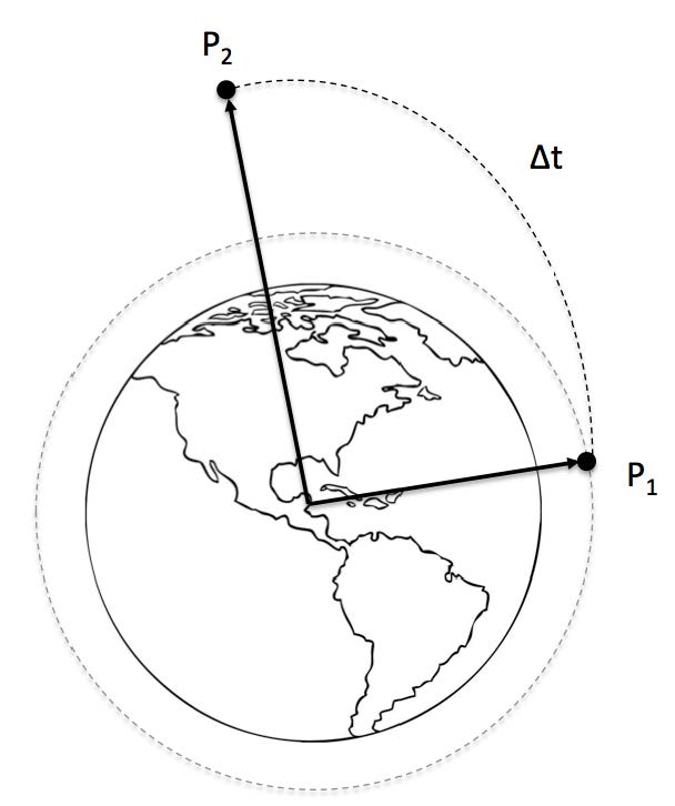
A key component of most mission trajectory planning is the solution of Lambert-type orbital boundary value problems (BVP). Specifically, the classic Lambert problem is a nonlinear BVP wherein a trajectory is sought that connects two points in space (Figure 1) subject to a specified constraint on the time-of-flight. Energy constraints may also be imposed as an alternative to the time-of-flight. Significant research has been devoted to the numerical solution of this nonlinear BVP over the years. In broad terms, the solution approaches can be categorized as those based on ‘geometric’ approaches and those employing ‘universal variable’ approaches. In the geometric approaches, the BVP is transformed into an equivalent Lambert equation (e.g., Reference [19]) involving orbital elements that is solved via iteration [20,21,22,23,24]. The direct geometry approaches are typically limited to elliptical orbits; furthermore, some approaches cited are restricted to a trajectory transfer angle of less than one orbit, whereas others may be extended to multiple revolutions. In contrast, the universal variable-based approaches were developed to provide numerical methods that are valid for all orbit conics (i.e., elliptical and hyperbolic. The universal variable approach is based on a transformation of the orbit anomalies to an auxiliary variable that leads to a new ‘universal’ time-of-flight equation [25]. Numerous methods for efficiently solving this transformed equation have been proposed [26,27,28,29,30].
In the present study, the evolutionary computing methodology of Differential Evolution (DE) is used to solve a class of ‘Lambert-type’ orbital boundary-value problems. The DE-based approach, in contrast to the methods described previously, directly solves the two-body equation of motion for the spacecraft by iterating on the initial velocity vector at (see Figure 1). As such, it is valid for all orbit conics. Perturbation effects of planetary oblateness and rarefied atmospheric drag are included in this study to reflect realistic conditions in low Earth orbit (LEO). The end condition of the arrival at may involve a simple positional requirement (intercept trajectory) or a positional and velocity requirement (rendezvous trajectory). Multiple objectives may include minimizing positional accuracy of the trajectory endpoint (i.e., relative to ), fuel consumption, and time-of-flight accuracy. In particular, the fuel constraint has historically represented a key limitation in orbit planning. In this work, we combine these objectives into a single weighted fitness function, with various weights depending on the particular problem being solved. The resulting fitness function thus represents a trajectory optimization problem.
This investigation consists of three essential parts. In the first part, we show that it is possible to recover classic solutions to Lambert’s problem for either (1) a specified time-of-flight or (2) a minimum energy orbital transfer, thus validating the evolved trajectories against known analytical results. In the second part, we evolve trajectories in the presence of orbital perturbations arising from the oblateness of the Earth and rarefied atmospheric drag for which there are no known analytical solutions. Lastly, the intercept problem is then extended to a multi-orbit scenario in which the only perturbing force is planetary oblateness. The capability of the Differential Evolution technique for solving Lambert’s problem with complex physics (perturbations) is demonstrated, suggesting that the DE-based method offers a viable option for realistic mission planning.
2. Overview of Governing Physics
A Newtonian gravitational potential is the canonical model used in orbital mechanics. In this model, gravity is assumed to be a spherically-symmetric, attractive force that is inversely proportional to the square of the distance between the centers of mass between two bodies. For problems involving a spacecraft and the Earth, the mass of the spacecraft is inconsequential and the gravitational constant is given by where G is the universal gravitational constant and is the mass of the Earth. The governing equation for the spacecraft motion relative to a frame centered at the Earth is given by
where is the position vector of the spacecraft from the Earth’s center and is the gravitational parameter defined above. In reality, many trajectories arising in actual mission planning are subject to non-negligible perturbation forces that result in non-Keplerian motion. For low Earth orbits (LEO), for example, two important perturbations are gravitational variations due to planetary oblateness and rarefied atmospheric drag. The mathematical form of these perturbations are included below for completeness.
2.1. Oblateness Perturbation in Low Earth Orbits (LEO)
The fact that the Earth is actually an oblate spheroid, as a consequence of its axial rotation, gives rise to an axisymmetric gravitational potential that can be formally expressed in terms of a series expansion of zonal spherically harmonics [31]. For the Earth, the oblateness perturbation can be well modeled by the addition of a single correction term, called the second zonal harmonic , to the spherically symmetric Newtonian potential. The corresponding perturbation acceleration is given by [31]:
where is the equatorial radius of the Earth and are unit vectors aligned in the directions of the Cartesian coordinate axes. Specifically, the vector is aligned with the north pole of the Earth’s rotation axis and the vector lies within the equatorial plane and points towards the First Point of Ares; the direction of the vector then immediately follows. The magnitude of this perturbation is zero at the equator and increases with latitude; furthermore, the magnitude is seen to diminish with the fourth-power of the altitude. Therefore, its effect is most pronounced for LEO scenarios and especially those with higher inclinations. A dynamical consequence of this perturbation is that a slow precession of the orbit results—that is, the orbit is no longer closed as in Keplerian motion. Although the precession rate is typically no more that a few degrees per orbit, over the span of many orbits, the impact of this perturbation effect becomes significant.
2.2. Rarefied Atmospheric Drag in LEO
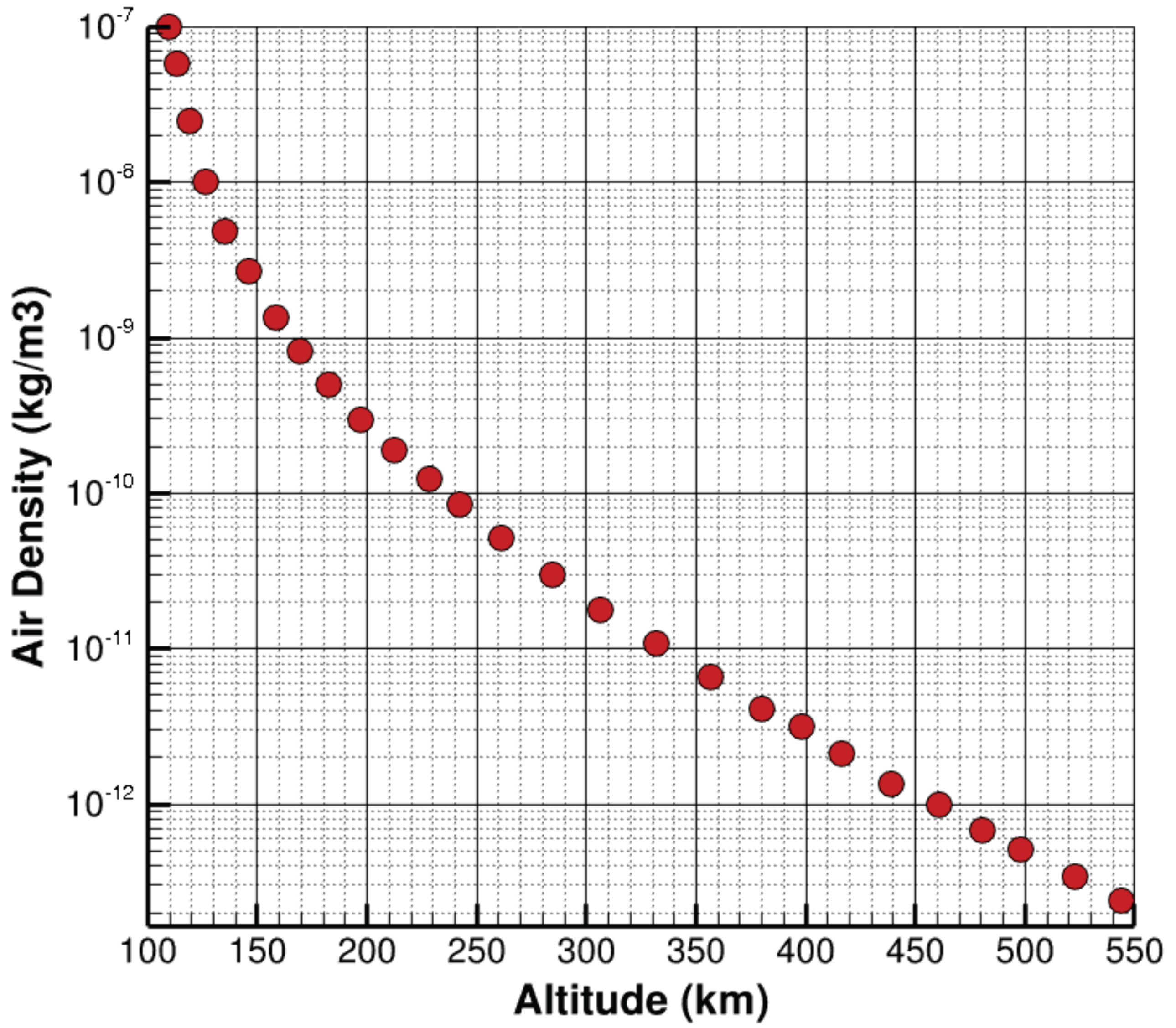
The so-called ‘Karman line’, defined to be at an altitude of 100 km above the Earth, is commonly regarded as the boundary between the Earth’s atmosphere and space. In reality, the density of the Earth’s atmosphere undergoes a significant decay beginning at an altitude of 20 km and a highly rarefied vestige of the atmosphere extends well beyond the Karman line and into the region of LEO, as illustrated in Figure 2. As a consequence, spacecraft in very low orbits are subject to a ballistic drag force from the residual atmosphere. While small in magnitude, the effect of atmospheric drag is to reduce the velocity of an orbiting object and, given sufficient time, leads to an orbital decay and eventual atmospheric reentry. A model of ballistic drag is typically employed to describe this effect and is given by [32]:
where is the altitude-dependent atmospheric density and B is the ballistic coefficient for the spacecraft geometry. The relative velocity is that between the spacecraft velocity and the atmospheric velocity at the instantaneous latitude:
where is the spacecraft velocity, is its position vector, and
is the angular velocity vector of the Earth’s rotation. As this effect is a retarding force, the acceleration is always negative and in the direction opposite of the current velocity. For a small spacecraft (‘nano sat’), which underlies the motivation for the present study, a typical value for the ballistic coefficient is [32].
3. Computational Methods
3.1. The Differential Evolution Algorithm
An evolutionary algorithm (EA) is a population-based, bio-inspired optimization method, modeled loosely after the process of evolutionary adaptation in biological systems [33]. Populations of candidate solutions (typically encoded as vectors of decision variables) undergo an iterative process of reproduction with variation, competition for limited space in the population, and fitness-based selection. Over iterations, the population evolves solutions that are increasingly fit. There are many flavors of EAs [33] that vary in the details of the algorithm. For example, genetic algorithms (GAs) rely primarily on discrete recombination of decision variables (a.k.a. crossover) to introduce new variation, so GAs work best when decision variables have small discrete alphabets and GAs require relatively large population sizes to ensure adequate sampling of the search space. On the other hand, differential evolution (DE) [34] was explicitly designed to work well with real-valued decision variables. DE primarily introduces new variation by computing weighted differences of existing candidate solutions and then adding scaled versions of these difference vectors to other existing candidate solutions. Thus, when individuals in the population are far from each other (as in an initially random population), the difference vectors are large and new candidate solutions sample the search space broadly (the so-called exploration phase of the evolution), but, as the better solutions are selected and the population begins to converge, the step sizes of the search become smaller and the algorithm automatically shifts to a more local search (the so-called exploitation phase of the evolution) to fine-tune the remaining solutions. DE is simple to implement, requires relatively small populations, has low computational overhead per generation, and performs well even in the presence of correlated decision variables and noise [13]. Consequently, DE has rapidly gained traction in the evolutionary computation community for real-valued optimization [35].
It is worthwhile to mention that another type of EA that is also well-suited to optimization of real-valued decision variables is covariance matrix adaptation evolution strategy (CMA-ES) [36]. However, in preliminary testing on other trajectory optimization problems [9], it was found that, while CMA-ES converged more quickly, it had a greater tendency to become trapped in local minima. In contrast, DE more consistently converged to the correct solutions. Thus, in this study, we opted to use a DE approach implemented within the Matlab software programming language (Matlab v2015b, Mathworks, Natick, MA, USA) with the source code available at http://www1.icsi.berkeley.edu/~storn/code.html).
3.2. Hybrid Evolutionary Approach
For this work, we have employed the form of DE originally developed by Price et al. [13]. For completeness, a brief summary of the algorithm is as follows. Suppose is a candidate solution vector in the current population. An intermediate vector () is created using three candidate solutions from the current population as
where the scaling factor is typically between 0 and 1. Next, a new candidate vector is formed by binary crossover process wherein each component of is randomly selected from either or based on a crossover probability . The original candidate is replaced by the newly constructed candidate in the next generation if the fitness is better than or equal to the fitness of . This procedure is repeated for all candidate solutions in the current generation. For all experiments reported here, we used a scaling parameter of , a crossover rate of = 0.8, and population size of , where M is the number of decision variables. These parameter settings were chosen based on limited preliminary experimentation using recommended ranges by Storn and Price [34].
The Differential Evolution method was used to find approximate solutions that fell within in the correct basin of attraction of the global optimum. Once the DE stage had terminated, the single best solution from the DE run was then refined using Matlab’s fminsearch function (a Nelder–Mead unconstrained nonlinear optimization method). The use of the gradient-based solver permitted more rapid convergence to an accurate solution once a potential solution was in the correct basin of attraction.
In general, the initial population was seeded using random distributions of the decision variables defined within a realistic range of values. However, in some non-Keplerian cases—notably Test Problem #4 (see below)—it was found that such an unrefined initial population led to poor success rates. For this case, a more strategic initial population was implemented so as to seed the population with better initial candidate solutions. Reasoning that the incorporation of LEO perturbations should not deviate dramatically from the unperturbed case, the initial velocity population could then be a statistical distribution about the classical Lambert solution. Specifically, the initial population was made by applying Gaussian noise of standard deviation 1 km/s to the corresponding unperturbed initial velocity vector. The standard deviation of 1 km/s was determined empirically as an acceptable value. If one selected a very small value of the deviation, this could overly restrict the initial population about a sub-optimum; in effect, this would operate counter to the notion of evolutionary optimization. On the other hand, too large of a value of the deviation might not sufficiently sample about the direct solution foregoing the intended benefit of this intuitive pre-population.
3.3. Test Problems
A set of five test problems was identified for the application of the evolutionary algorithm. Described below, these problems consist of both Keplerian motion, for which analytical solutions exist, and non-Keplerian motion:
- Problem 1:
- Classical Lambert Problem for a Given Time of Flight. In this problem, only Keplerian physics are considered, resulting in an idealized two-body problem. The goal is to minimize positional error at the target point for some pre-specified time of flight . Only the initial velocity vector is evolved. The exact analytical solution for this problem is known.
- Problem 2:
- Minimum Energy Lambert Transfer Ellipse. This is a variation of Problem #1 except that, in this case, the goal is to minimize the amount of energy necessary associated with the transfer ellipse from to . Here, the time of flight along the desired trajectory is not know a priori, thus both the initial velocity vector and the time of flight are evolved. The exact analytical solution for this problem is also known.
- Problem 3:
- Intercept Trajectory Accounting for Oblateness and Drag. In this non-Keplerian version of Problem #1, perturbations are introduced through the inclusion of the correction for non-spherical oblateness of the Earth Equation (2) as well as the correction for atmospheric drag Equation (3). The time of flight is specified, so only the initial velocity vector is evolved. The goal is to minimize positional error at for some pre-specified time of flight . No analytical solution exists for this problem.
- Problem 4:
- Multi-Orbit Intercept Trajectory Accounting for Oblateness. In this problem, the Keplerian orbit is perturbed through the inclusion of a gravitational correction for non-spherical oblateness of the Earth. A pre-specified time of flight is imposed that will require the spacecraft to complete multiple orbits of the Earth before reaching the target position. Here, we considered instances of 5-orbit, 20-orbit, and 100-orbit intercepts that hereafter will be referred to as Problems #4a, #4b and #4c, respectively. This was chosen to examine the computational success rate for two different levels of oblateness perturbation, with the effect growing with the number of orbits. While perturbations due to atmospheric drag could be included as incorporated as in Test Problem #3, when drag is present, it is impossible to guarantee that a trajectory exists that will reach the target without entering the Earth’s atmosphere. Thus, in this proof-of-concept study where we wish to quantify how often we can find a correct solution, we neglected perturbations due to atmospheric drag for this problem to ensure that a solution existed. The time of flight is specified, so only the initial velocity vector is evolved. The goal is to minimize positional error at for some pre-specified time of flight. No analytical solution exists for this problem. As discussed in Section 3.2, experiments with both ‘random’ and ‘strategic’ initial populations were performed.
3.4. Fitness Functions
A fitness function must be evaluated at each stage of the evolutionary process to evaluate the ‘quality’ of the current generation. The particular form of the fitness function is, of course, dependent on the objectives and constraints of the specific problem. Recalling that the problem being solved is that of a nonlinear boundary value problem, there were two essential forms of the fitness function used in this study. For cases where a specified time-of-flight is given, the ‘fitness function’ defaults to minimizing the positional error of the trajectory at the terminal location. In cases where the energy of the orbital maneuver is to be minimized, the fitness function will involve the magnitudes of the velocities at the endpoints of the trajectory.
Lambert Intercept Problems #1–4. The final position of the spacecraft is estimated by integrating the governing equations using a Runge–Kutta method with variable time step (Matlab’s ODE45 function) based on the evolved initial velocity vector and the prescribed or evolved time-of-flight . Because the fitness function is necessarily based on this simulation of flight trajectories, the time required to evaluate fitness is proportional to the time of flight of the trajectory being simulated, which varies for different individuals in the population. We created a single objective fitness function f to be minimized by weighting multiple objectives as follows:
In the above, are the weights for each term and denotes the 2-norm of the vector (Euclidean distances between estimates and targets). The quantity represents the positional error relative to the target location . The square of the necessary change in velocity relative to the initial velocity is proportional to the amount of energy required to change the velocity of the spacecraft for the new trajectory. The final term is a crash penalty, where is the maximum depth of below the surface of the Earth (this term is only non-zero when the spacecraft has crashed, and helps provide a gradient back to the feasible region). The values of the three weights vary with the particular test problem (and are sometimes zero), as described in Section 3.5.
3.5. Numerical Experiments
3.5.1. Lambert Intercept Cases (Problems #1–4)
For all experiments in Problems #1–4 reported here, we used the same initial and final locations, and . Centering a three-dimensional Cartesian coordinate system at the center of the Earth, the initial position was specified to be km. This places the spacecraft approximately 122 km above the surface of the Earth, a value for a very low Earth orbit. The final position was specified to be km, which has a classical Lambert solution of km/s, for a specified time of flight min (used in Problems #1 and #3). For Problems #4a and #4b, the times of flight are min and min, which forces the trajectory to orbit the Earth five and twenty times, respectively, before arriving at the target location . For Problem 2, the ending velocity vector is specified as and the evolving is prevented from going negative; note that is not needed for the other Problems #1,3,4. Appropriate values for the weights were determined empirically, since accurate normalization of the ranges of the terms was not found to be possible. Note that we have set some weights to zero so that not all terms are used in all test problems. This parametric data is summarized in Table 1.
The test problems were each run for 12 repetitions from different initial random populations. The rationale was to demonstrate the viability of the DE method to yield an acceptable solution to the problem given a limited number of attempts. Using a small batch of simulations also better emulates the method’s use in practical applications. The intention here was not to generate statistics for the expected outcomes based on a large set of runs.
The Problems #4a, 4b and #4c also used initial populations based on classical Lambert solutions. Typical DE runs were allocated a maximum CPU time before automatic termination of unsuccessful or stagnating cases; however, successful runs were allowed to terminate early if either (i) the maximum absolute error of any dimension in the evolving estimate of the initial velocity vector was less than km/s (for those cases where the true was known) or (ii) fitness f fell below . For the simulations involving five or less orbits (Problems #1–4a), a default time limit of 20 min of CPU was used and found to be a conservative value, as all cases were found to terminate via other stopping criteria. In the cases of Problem #4b and #c, with the 20-orbit and 100-orbit intercept requirements, a greater CPU time limit was necessary since these cases were more computationally intensive. As the appropriate CPU time limit was not known a priori, simulations were run and results examined for different time limits. In Problem #4b, time limits of 20 min and 60 min were tested, and, for Problem #4c, time limits of 120 min and 180 min were used. In the latter case, the 180 min runtime results did not improve significantly over the 120 min results, indicating that the difficulty in trials of 120 min and greater lies in the problem and not in the evolution being stopped prematurely. We then applied fminsearch to the best evolved solution for 200 iterations (with all tolerances and other options left at the default settings). A trial was considered successful if the final best solution was within 1 m of the target location (this is a conservative criterion for real LEO missions).
For the DE, we used a scaling parameter , a crossover rate of , and population size of , where M is the number of objective variables. These parameter settings were chosen based on limited preliminary experimentation using recommended ranges in [13]. For example, we experimented with crossover rates between and in increments of and found that performed the best for this problem (gave lower fitnesses in a shorter amount of time). We also experimented with population sizes N based on using either five or ten individuals per gene, but did not see appreciable differences in resulting fitnesses and so went with the smaller population sizes.
4. Results
Upon examination of the results, three types of results were apparent: (i) infeasible trajectories that ended up at but that intersected the Earth (this occurred only once, for Problem #1), (ii) trajectories that ended up hundreds or thousands of km from (this occurred in 7 of the 12 trials of the multi-orbit Problem #4a without Lambert-based initialization), and (iii) feasible trajectories that ended close to the target location (in all but one case, these were much less than 1 m from the target and were therefore considered successful trials).
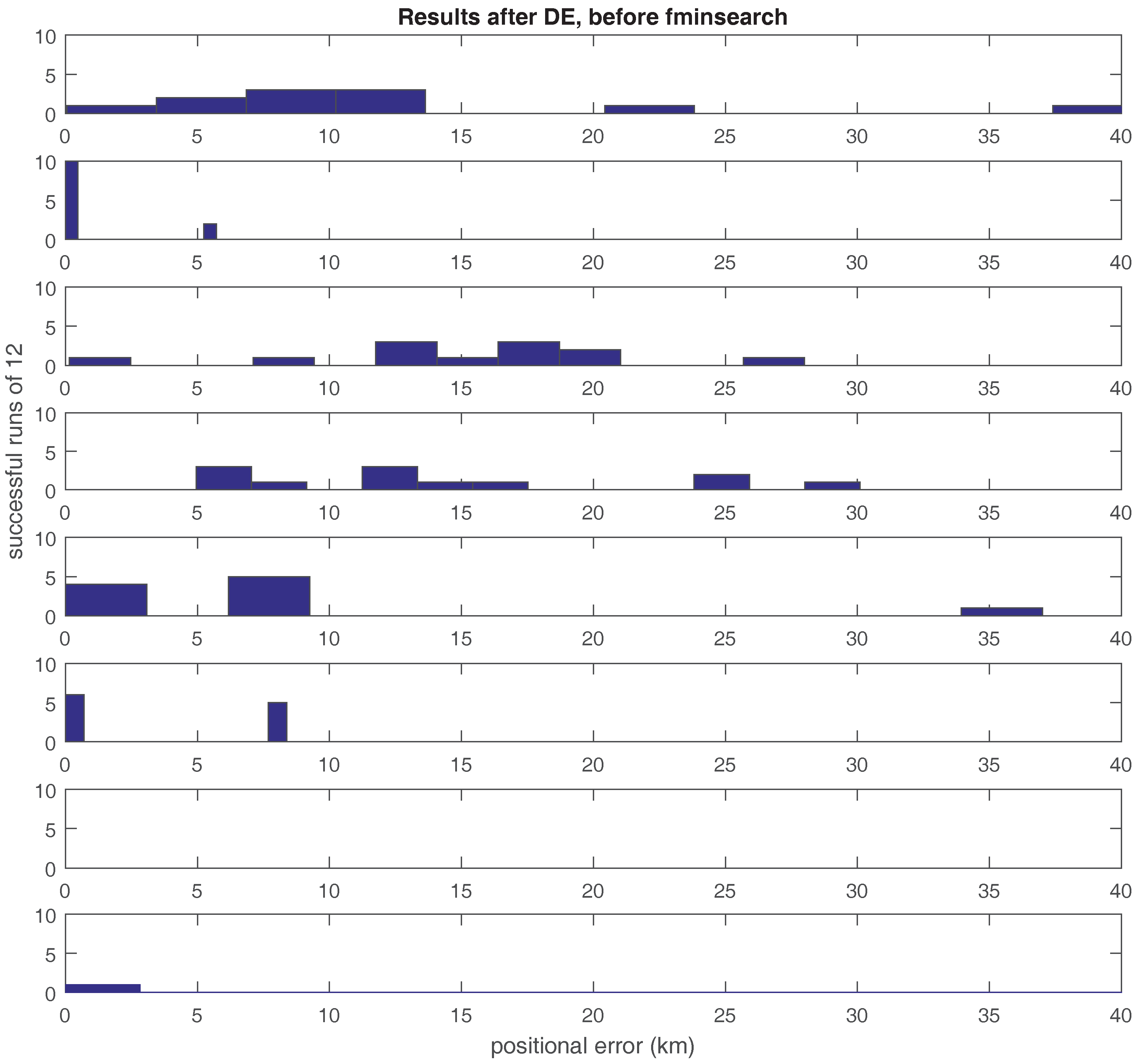
Histograms of the positional error
are shown in Figure 3 for all solutions after the DE phase and without refinement (i.e., before fminsearch) that were within 40 km of the target. Note that Problem #4b data for the 20 min and 60 min run times and Problem #4c data for the 60 min and 120 min run times are also included. For comparison, Figure 4 shows solution meters of the target after refinement using fminsearch to highlight the improvement yielded by the hybrid evolutionary approach. The histograms of Figure 3 and Figure 4 reflect random initialization of the populations. For more complicated multi-orbit intercept cases, the value of the Lambert-based population initialization is apparent when applied to the five-orbit intercept case (Figure 5).
Quantitative results for all successful runs of DE + fminsearch are summarized in Table 2. The positional errors represent the average Euclidean distance (in m) between and for all successful runs. For Problems #1–3, we were able to find successful solutions in all but two trials (see Table 2). In the one unsuccessful trial for Problem #1, the solution was in a local optimum that sent the spacecraft on a trajectory through the Earth (note that this could have been precluded if we had explicitly formulated the fitness function to guard against such trajectories, but we opted to check for this in post-processing rather than further slow down the fitness function). In the one trial considered unsuccessful for Problem #2, the final positional error was still only 4.6 m from the target; this level of error may actually be within tolerance, depending on the mission, and probably could have been further reduced with additional iterations of fminsearch, although we did not try the latter. For the more difficult multi-orbit Problems #4a and #4b, we were still able to find successful solutions in the majority of the cases: 100% for a five-revolution intercept with Lambert-based initialization and over 50% for a twenty-orbit intercept. Note also from Table 2 that increasing the CPU time for the twenty-orbit intercept increased the success rate from 42% to 58%. For Problem #4c, the lack of successful runs for the 20 min time limit is indicative of that time being insufficient for this implementation (Matlab) to find solutions within a basin of attraction for a successful run; the DE solutons would also have to be sufficiently close such that their placement allowed the fminsearch to find the successful run.
If one views the 12 trials as restarts, the best solutions found are quite impressive, as summarized in the rightmost column of Table 2. Here, it can be seen that final positional errors of the best solutions found were negligible. For Problem #1, the analytical solution for the initial velocity was recovered to within nine decimal places of accuracy (in km/s), and, for Problem #2 the analytical solution for the optimal time-of-flight was recovered to within 4.8 s.
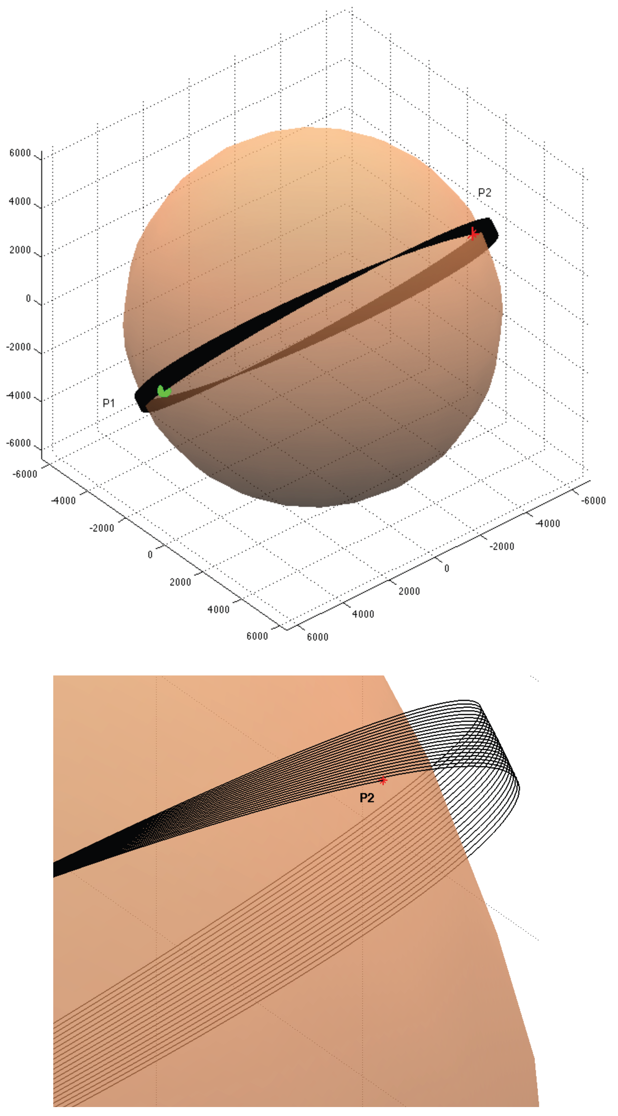
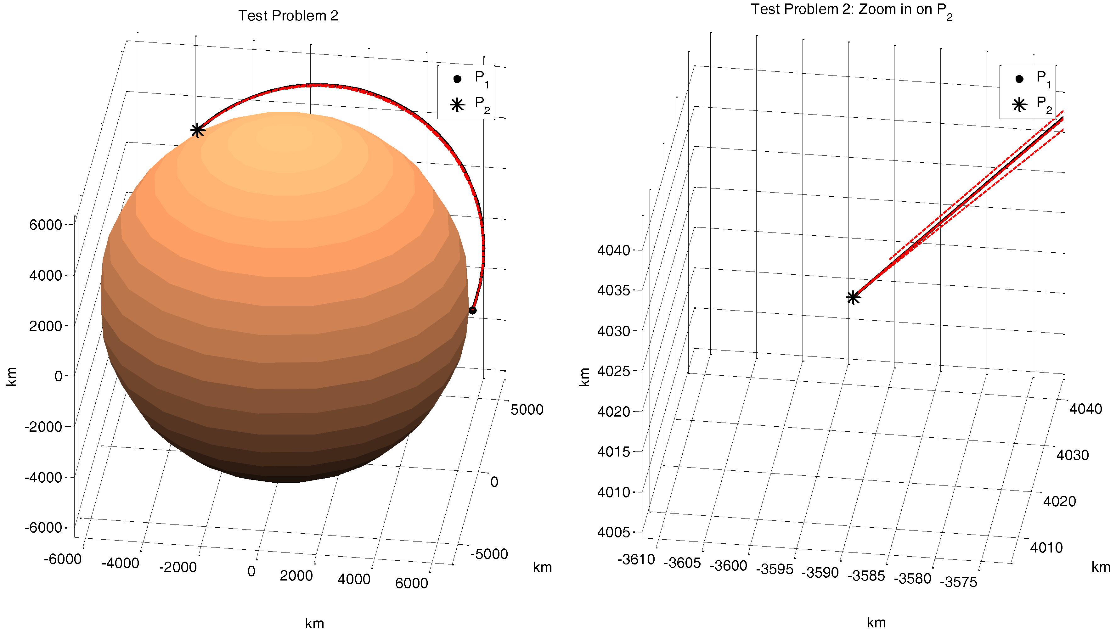
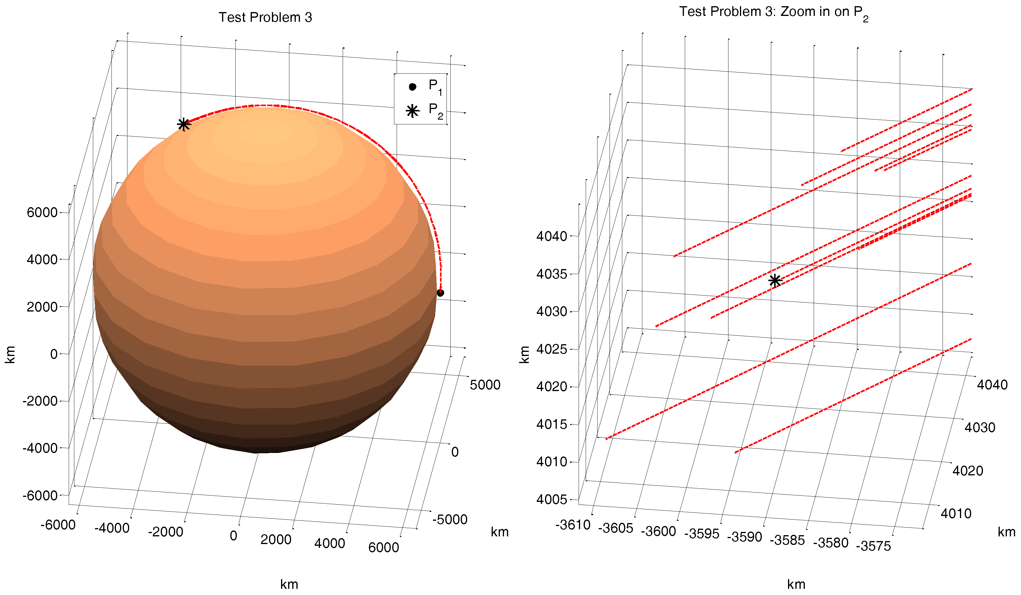
The corresponding trajectories for all successful runs for Problems #1–3 appear in Figure 6, Figure 7 and Figure 8, respectively. In some cases, trajectories lie on top of each other and are not visually distinguishable. The right-hand panels of Figure 6, Figure 7 and Figure 8 show close-ups of the successful trajectories after DE but before refinement with fminsearch (note the zoomed in scales of the axes). After refinement with fminsearch, the successful trajectories are all <0.3 m from the target, so they would appear indistinguishable on these figures. For Problem #4a, we show all five orbits of only the single best trajectory in Figure 9; note the precession of the orbits toward the target point . The precession is even more noticeable in the trajectory for the twenty-orbit intercept of Problem #4b (Figure 10).
5. Discussion
The focus of this study has been to investigate the utility of a DE-based approach for spacecraft trajectory planning under the realistic orbital conditions that would be present in the LEO and Earth–Moon system environments. With this in mind, it is appropriate to examine both the performance and limitations of the present model within the context of actual mission planning performed by space agencies such as NASA.
5.1. Traditional Mission Planning Approaches
Historically, the computational design of mission trajectories has been based on problem-specific algorithms that employed classical numerical approaches for orbital mechanics (e.g., boundary-value problems [37]). Within the past decade or so, however, there has been an effort to develop more generalized and robust trajectory design approaches including optimization. Johnson et al. [38] developed the Copernicus program for NASA Johnson Space Center that incorporated many existing case-specific NASA trajectory codes into a single mission design and optimization tool. Beginning in the 1990s, modern dynamical systems approaches using invariant manifolds were introduced for mission planning in perturbed systems [39]; this approach was realized in mission planning for the NASA Genesis mission launched in 2001 [40]. Most recently, NASA Goddard Space Flight Center has introduced the Evolutionary Mission Trajectory Generator software, which designs and optimizes complex interplanetary trajectories involving multiple planetary flybys using a GA [41]. However, to date, these methods have largely focused on planning orbital trajectories for problems where near-Earth perturbations are negligible.
With the recent increase in small satellites in LEO (e.g., ‘cubesats’ and ‘nanosats’), as well as formation-flying mission architectures, it is important to extend automated design approaches to include realistic LEO perturbations. The current study serves as proof-of-concept that DE can be effective in automating accurate LEO trajectory planning, which represents a new contribution to the current astrodynamics literature.
5.2. Trajectory Accuracy
In real LEO maneuvers, the required positional accuracy for modern trajectory planning is on the order of meters [42]. Of course, the specific error tolerance is necessarily dependent on the particular mission. In the results presented here, all successful runs had positional errors of less than 0.3 m (with best runs out of 12 trials within 0.01 m of the target position) for all four problems (Table 2); these positional errors are well within the required tolerances for LEO missions.
5.3. Opportunities for Model Improvement
Although the computational model presented in this work has incorporated a number of realistic and important perturbations for LEO maneuvers, there remain opportunities for further improvement, including: (a) incorporating additional perturbations; (b) solving more difficult LEO problems, such as multi-impulse, trajectories, continuous thrust trajectories, and multi-spacecraft swarm trajectories; (c) evolving Pareto sets of non-dominated solutions with respect to the multiple objectives; and (d) trajectory design applied to formation-flying of multiple satellites. We discuss these areas below.
There are two particular sources of perturbation that are not accounted for in the present model. The first is the effect of solar radiation (photon) pressure, which can either accelerate or decelerate the spacecraft depending on its orientation. For very low orbits, this effect is small compared to atmospheric drag; however, for higher orbits, the reverse is true. The second source of perturbation is caused by gravitational effects of the Sun. This effect is negligible for LEO scenarios but may be relevant for higher orbits (e.g., geosynchronous orbits, GEO) and within the Earth–Moon system. Therefore, to extend the capabilities of the current framework beyond LEO, the inclusion of solar gravity may be appropriate.
The current version of the model is restricted to trajectories produced by a single initial impulse. While this is acceptable for preliminary orbit design, it excludes the possibility of mid-course correction(s) to account for perturbation effects. A more flexible and realistic approach would be to allow for a finite number of impulses during the trajectory. One could also allow for the possibility of a continuous thrust trajectory, where the spacecraft produces a thrust during the entire maneuver. Continuous thrust maneuvers are consistent with spacecraft utilizing electric propulsion systems (e.g., ion engines) as well as solar sails.
Another area of interest is the design of trajectories of small constellations of LEO spacecraft flying together; these spacecraft must not only reach a particular target area, but must also remain within certain distances of each other and, in some cases, maintain specific formations. One contemporary example is NASA’s Magnetospheric Multi-Scale (MMS) mission consisting of four satellites flying in a tetrahedral configuration at the measurement site in the orbit [1]. Efforts on the use of DE applied to such topological problems have reported in recent works by our group [10,43,44,45].
In the current approach, we chose to combine the multiple objectives into a single weighted fitness function, and have emphasized trajectory planning where the primary objective is either time-of-flight or fuel considerations. Realistic mission planning could benefit from a multi-objective version of DE (e.g., [46]) that returns a relatively uniformly spaced set of non-dominated solutions. Mission planners could then consider the trade-offs between the various objectives and constraints in selecting an appropriate trajectory to implement.
In the study described here, the numerical model was implemented in the Matlab programming software. This selection was made for expediency and without any attempt to improve and/or optimize the code for speed. A CPU time limit of 20 min was imposed for all cases except those with multiple revolutions; this time limit corresponded to approximately 12,500 generations being rendered. Within the context of actual mission planning, this represents an insignificant amount of computation time. Nonetheless, improving the efficiency of the code (e.g., converting to a language such as C/C++) would likely prove beneficial when coupling the simulations to a higher-order ordinary differential equation solver or a higher fidelity forward trajectory simulator, such as NASA’s publicly available GMAT code (http://gmat.gsfc.nasa.gov).
6. Conclusions
In this study, Differential Evolution (DE) was investigated as a tool for solving a class of nonlinear orbital boundary value problems—Lambert’s Problem—with time or energy constraints. The accuracy of the technique was first demonstrated in two different test cases involving Keplerian orbits that could be benchmarked against known solutions. The method was then applied to single and multi-revolution cases involving non-Keplerian orbits arising from oblateness and rarefied atmospheric drag perturbations.
The hybrid DE evolutionary approach was found to be very promising in that it was rarely trapped in local optima and was often able to get sufficiently close to the error-minimizing trajectory such that subsequent refinement with Nelder–Mead optimization was able to reduce final positional errors to within mission tolerance. For this study, the positional error was set to 0.3 m, which is well within the acceptable tolerance for real LEO mission planning. In more challenging problems, such as the multi-orbit problem studied here, it was found that multiple restarts may be required; however, even in this difficult problem, a success rate of 58% was achieved.
In this method, only the initial velocity and possibly time of flight are evolved. As such, additional complex perturbation effects can be readily incorporated into fitness evaluation without affecting the remainder of the evolutionary code demonstrated, suggesting that the DE-based method offers a viable option for realistic mission planning. We therefore conclude that a hybrid method using DE to find the global basin of attraction, followed by refinement with a local optimization method such as Nelder–Mead to hone in on the global optimum, is a promising approach to mission design and optimization of LEO and related trajectories.
Acknowledgments
This work has been supported by the Vermont Space Grant under NASA Cooperative Agreement #NNX10AK67H, with additional computing support from the Vermont Advanced Computing Center (NASA Cooperative Agreement #NNX06AC88G). The authors are grateful to Jacob Englander of NASA Goddard Space Flight Center for helpful discussions and comments.
Author Contributions
D.W.H. and D.L.H. conceived and designed the computational project; D.W.H. wrote the numerical algorithms and performed the computations; D.W.H. and D.L.H. analyzed the data and co-authored this manuscript.
Conflicts of Interest
The authors declare no conflict of interest.
Abbreviations
The following abbreviations are used in this manuscript:
| DE | Differential Evolution |
| EA | Evolutionary Algorithms |
| GA | Genetic Algorithms |
| LEO | Low Earth Orbit |
References
- NASA’s Magnetospheric Multi-Scale Mission. Available online: http://mms.gsfc.nasa.gov (accesed on 9 September 2017).
- Taini, G.; Amorosi, L.; Notarantonio, A.; Palmerini, G.B. Applications of genetic algorithms in mission design. In Proceedings of the 2005 IEEE Aerospace Conference, Big Sky, MT, USA, 5–12 March 2005. [Google Scholar]
- Englander, J.A.; Conway, B.A.; Williams, T. Automated Mission Planning via Evolutionary Algorithms. J. Guid. Control Dyn. 2012, 35, 1878–1887. [Google Scholar] [CrossRef]
- Vinko, T.; Izzo, D. Global Optimisation Heuristics and Test Problems for Preliminary Spacecraft Trajectory Design. In Technical Report; European Space Agency: Paris, France, 2008. [Google Scholar]
- Vavrina, M.; Englander, J.; Ghosh, A. Coupled Low-Thrust Trajectory and Systems Optimization Via Multi-objective Hybrid Optimal Control. In Proceedings of the AAS/AIAA Space Flight Mechanics Meeting, Williamsburg, VA, USA, 11–15 January 2015. [Google Scholar]
- Cassioli, A.; Izzo, D.; Di Lorenzo, D.; Locatelli, M.; Schoen, F. Global Optimization Approaches for Optimal Trajectory Planning. In Modeling and Optimization in Space Engineering; Springer Optimization and Its Applications; Fasano, G., Pintér, J.D., Eds.; Springer: New York, NY, USA, 2013; Volume 73, pp. 111–140. [Google Scholar]
- Vasile, M.; Minisci, E.; Locatelli, M. An Inflationary Differential Evolution Algorithm for Space Trajectory Optimization. IEEE Trans Evol. Comput. 2011, 15, 267–281. [Google Scholar] [CrossRef] [Green Version]
- Izzo, D.; Simoes, L.; Martens, M.; de Croon, G.; Heritier, A.; Yam, C.H. Search for a Grand Tour of the Jupiter Galilean Moons. In Proceedings of the 15th Annual Conference on Genetic and Evolutionary Computation, Amsterdam, The Netherlands, 6–10 July 2013; pp. 1301–1308. [Google Scholar]
- Hinckley, D.; Zieba, K.; Hitt, D.L.; Eppstein, M.J. Evolved spacecraft trajectories for low earth orbit. In Proceedings of the 2014 Annual Conference on Genetic and Evolutionary Computation, Vancouver, BC, Canada, 12–16 July 2014. [Google Scholar]
- Hinckley, D.; Hitt, D.; Eppstein, M. Evolutionary Optimization of Satellite Formation Topology over a Region of Interest. In Proceedings of the AIAA Guidance, Navigation, and Control Conference, Kissimmee, FL, USA, 5–9 January 2015. [Google Scholar]
- Cacciatore, F.; Toglia, C. Optimization of Orbital Trajectories Using Genetic Algorithms. J. Aerosp. Eng. Sci. Appl. 2008, 1, 58–69. [Google Scholar] [CrossRef]
- Lee, S.; von Allmen, P.; Fink, W.; Petropoulos, A.E.; Terrile, R.J. Multi-Objective Evolutionary Algorithms for Low-Thrust Orbit Transfer Optimization. In Proceedings of the Genetic and Evolutionary Computation Conference, Washington, DC, USA, 25–29 June 2005. [Google Scholar]
- Price, K.; Storn, R.; Lampinen, J. Differential Evolution: A Practical Approach to Global Optimization; Springer: Berlin, Germany, 2006. [Google Scholar]
- Bessette, C.R.; Spencer, D.B. Optimal Space Trajectory Design: A Heuristic-Based Approach. Adv. Astronaut. Sci. 2006, 124, 1611–1628. [Google Scholar]
- Hansen, N. The CMA evolution strategy: A comparing review. StudFuzz 2006, 192, 75–102. [Google Scholar]
- Casalino, L.; Sentinella, M.R. Evolutionary Algorithm for Interplanetary Trajectories Optimization. Astrocon 2008, 2008. [Google Scholar]
- Olds, A.D.; Kluever, C.A.; Cupples, M.L. Interplanetary Mission Design Using Differential Evolution. J. Spacecr. Rockets 2007, 44, 1060–1070. [Google Scholar] [CrossRef]
- Vasile, M.; Locatelli, M. A hybrid multiagent approach for global trajectory optimization. J. Glob. Optim. 2009, 44, 461–479. [Google Scholar] [CrossRef] [Green Version]
- Prussing, J.E.; Conway, B.A.; Prussing, J.E. Orbital Mechanics; Oxford University Press: New York, NY, USA, 1993; Volume 57, p. 208. [Google Scholar]
- Escobal, P. Methods of Orbit Determination; R.E. Krieger Publishing Company: Malabar, FL, USA, 1976. [Google Scholar]
- Ochoa, S.I.; Prussing, J.E. Multiple revolution solutions to Lambert’s Problem. In Spaceflight Mechanics 1992; Diehl, R.E., Schinnerer, R.G., Williamson, W.E., Boden, D.G., Eds.; American Astronautical Society: Colorado Springs, CO, USA, 1992; pp. 1205–1216. [Google Scholar]
- Avanzini, G. A Simple Lambert Algorithm. J. Guid. Control Dyn. 2008, 31, 1587–1594. [Google Scholar] [CrossRef]
- He, Q.; Li, J.; Han, C. Multiple-revolution solutions of the transverse-eccentricity-based lambert problem. J. Guid. Control Dyn. 2010, 33, 265. [Google Scholar] [CrossRef]
- Thorne, J.D. Lambert’s theorem-A complete series solution. J. Astronaut. Sci. 2004, 52, 441–454. [Google Scholar]
- Battin, R. An Introduction to the Mathematics and Methods of Astrodynamics; AIAA Education Series; American Institute of Aeronautics and Astronautics: Reston, VA, USA, 1987. [Google Scholar]
- Lancaster, E.; Blanchard, R.; Aeronautics, U.S.N.; Administration, S.; Center, G.S.F. A Unified Form of Lambert’s Theorem; Technical Note; National Aeronautics and Space Administration: Washington, DC, USA, 1969.
- Bate, R.; Mueller, D.; White, J. Fundamentals of Astrodynamics; Dover Books on Aeronautical Engineering Series; Dover Publications: Mineola, NY, USA, 1971. [Google Scholar]
- Gooding, R.H. A procedure for the solution of Lambert’s orbital boundary-value problem. Celest. Mech. Dyn. Astron. 1990, 48, 145–165. [Google Scholar]
- Arora, N.; Russell, R.P. A gpu accelerated multiple revolution Lambert solver for fast mission design. In Proceedings of the AAS/AIAA Space Flight Mechanics Meeting, New Orleans, LA, USA, 13–17 February 2011; pp. 10–198. [Google Scholar]
- Izzo, D. Revisiting Lambert’s problem. Celest. Mech. Dyn. Astron. 2015, 121, 1–15. [Google Scholar] [CrossRef]
- Schaub, H.; Junkins, J.L. Analytical Mechanics of Space Systems; AIAA: Reston, VA, USA, 2003; p. 794. [Google Scholar]
- Wong, J.; Reed, H.; Ketsdever, A. University micro-/nanosatellite as a micropropulsion testbed. Micropropuls. Small Spacecr. 2000, 187, 25. [Google Scholar]
- Eiben, A.; Smith, J.E. Introduction to Evolutionary Computing; Springer: New York, NY, USA, 2003. [Google Scholar]
- Storn, R.; Price, K. Differential evolution—A simple and efficient heuristic for global optimization over continuous spaces. J. Glob. Optim. 1997, 11, 341–359. [Google Scholar] [CrossRef]
- Das, S.; Suganthan, P.N. Differential Evolution: A Survey of the State-of-the-Art. IEEE Trans. Evol. Comput. 2011, 15, 4–31. [Google Scholar] [CrossRef]
- Hansen, N.; Ostermeier, A. Completely derandomized self-adaptation in evolution strategies. Evol. Comput. 2001, 9, 159–195. [Google Scholar] [CrossRef] [PubMed]
- Farquhar, R.W.; Muhonen, D.P.; Newman, C.R.; Heubergerg, H.S. Trajectories and Orbital Maneuvers for the First Libration-Point Satellite. J. Guid. Control Dyn. 1980, 3, 549–554. [Google Scholar] [CrossRef]
- Johnson, G.; Munoz, S.; Lehman, J. Copernicus: A Generalized Trajectory Design and Optimization System. In Technical Report; University of Texas: Austin, TX, USA, 2003. [Google Scholar]
- Howell, K.; Barden, B.; Lo, M. Application of Dynamical Systems Theory to Trajectory Design for a Libration Point Mission. J. Astronaut. Sci. 1997, 45, 161–178. [Google Scholar]
- Lo, M.; Williams, B.; Bollman, W.; Han, D.; Corwin, R.; Hong, P.; Howell, K.; Barden, B.; Wilson, R. Genesis Mission Design. J. Astronaut. Sci. 2001, 49, 169–184. [Google Scholar]
- Englander, J. Automated Trajectory Planning for Multiple-Flyby Interplanetary Missions. Ph.D. Thesis, University of Illinois, Champaign, IL, USA, 2013. [Google Scholar]
- Englander, J.; NASA Goddard Space Flight Center, Greenbelt, MD USA. Personal communication, 2015.
- Hinckley, D.; Hitt, D. Evolutionary Optimization of a Rendezvous Trajectory for a Satellite Formation with a Space Debris Hazard. In Proceedings of the AAS/AIAA Astrodynamics Specialist Conference, Vail, CO, USA, 9–15 August 2015. [Google Scholar]
- Hinckley, D.; Hitt, D. Two-Impulse Evolutionary Optimization of Satellite Formations with Topological Constraints. In Proceedings of the 26th AAS/AIAA Space Flight Mechanics Meeting, Napa, CA, USA, 14–18 February 2016. [Google Scholar]
- Hinckley, D.; Hitt, D. Two-Impulse Evolutionary Optimization of Satellite Formations Over Multiple Revolutions with Topological Constraints. In Proceedings of the 9th International Workshop on Satellite Constellations and Formation Flying, Boulder, CO, USA, 19–21 June 2017. [Google Scholar]
- Chichakly, K.J.; Eppstein, M.J. Improving Uniformity of Solution Spacing in Biobjective Evolution. In Proceedings of the Genetic and Evolutionary Computation Conference (GECCO), Amsterdam, The Netherlands, 6–10 July 2013; pp. 87–88. [Google Scholar]
Figure 1.
Schematic diagram of the classical Lambert problem involving the orbital transfer from an initial position to a new location with a prescribed time-of-flight .
Figure 1.
Schematic diagram of the classical Lambert problem involving the orbital transfer from an initial position to a new location with a prescribed time-of-flight .
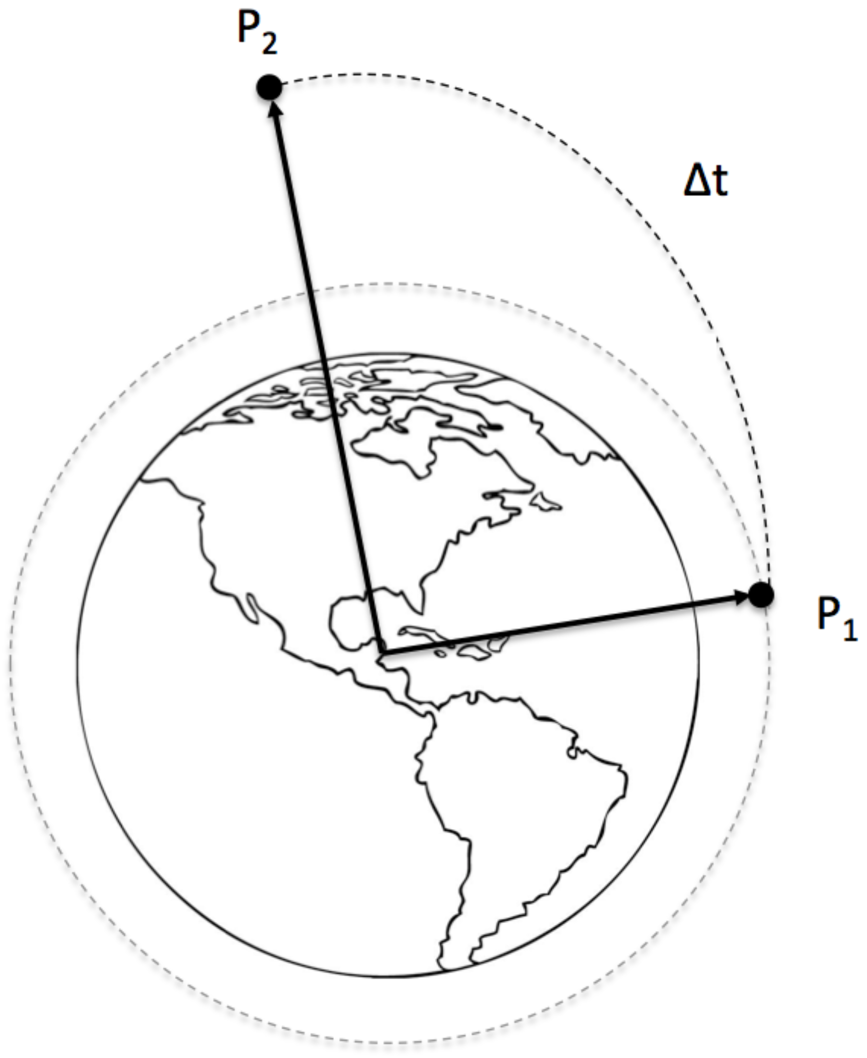
Figure 2.
Atmospheric density data showing a power-law decay with altitude. The data shown was extracted from Wong et al. [32].
Figure 2.
Atmospheric density data showing a power-law decay with altitude. The data shown was extracted from Wong et al. [32].

Figure 3.
Histograms of the positional error (in km) in the test Problems #1–4 after differential evolution (DE) but before refinement with fminsearch, for all trials that were within 40 km of the target after DE. There were 12 trials performed for each of the test problems.
Figure 3.
Histograms of the positional error (in km) in the test Problems #1–4 after differential evolution (DE) but before refinement with fminsearch, for all trials that were within 40 km of the target after DE. There were 12 trials performed for each of the test problems.

Figure 4.
Histograms of the positional error (in m) in the test Problems #1–4 after DE followed by refinement with fminsearch.
Figure 4.
Histograms of the positional error (in m) in the test Problems #1–4 after DE followed by refinement with fminsearch.
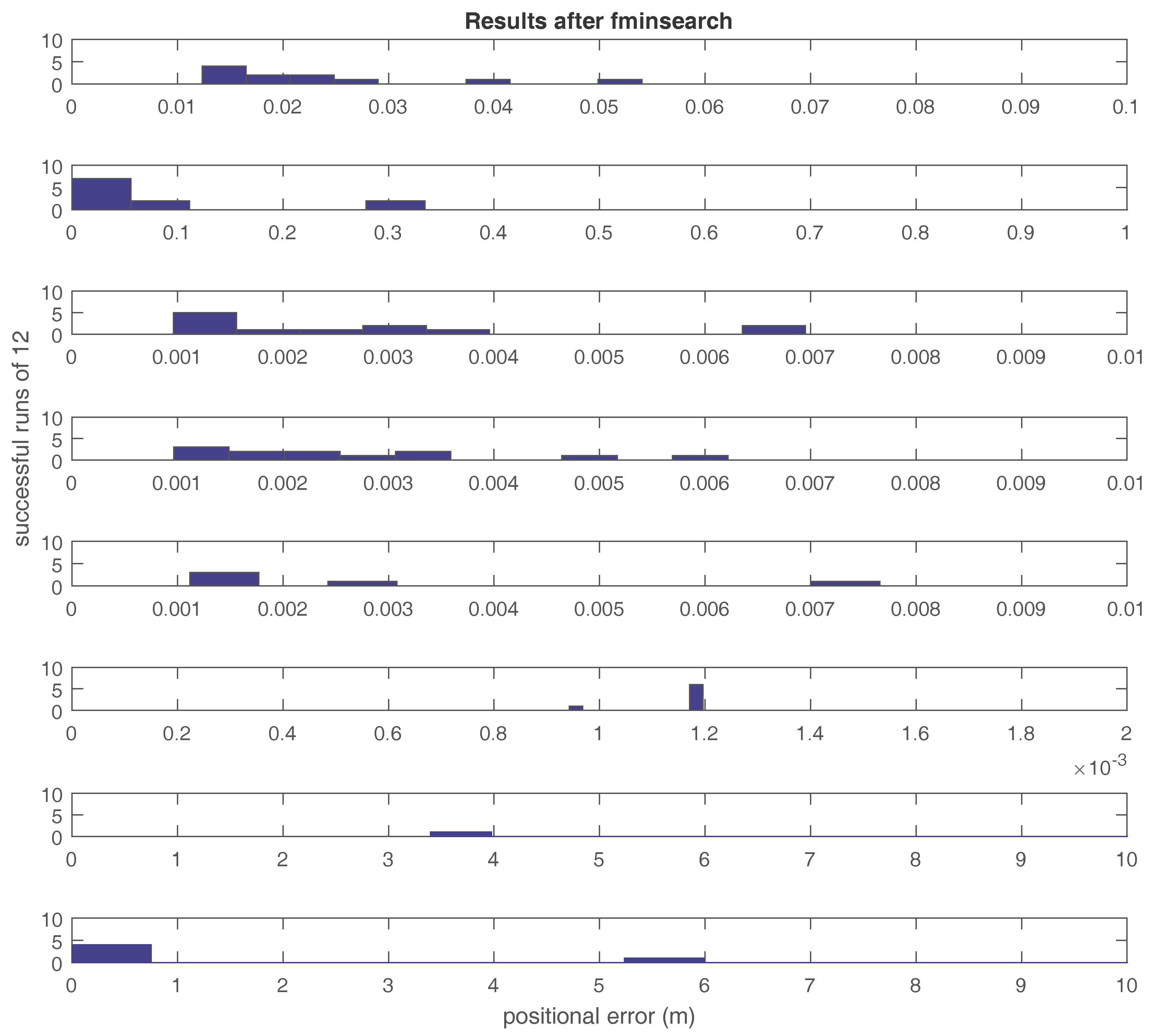
Figure 5.
Histograms of the positional error (in mm) in the test Problem #4a showing the improvement in success rate between random population initialization (top) and initial population based on the Lambert solution (bottom).
Figure 5.
Histograms of the positional error (in mm) in the test Problem #4a showing the improvement in success rate between random population initialization (top) and initial population based on the Lambert solution (bottom).
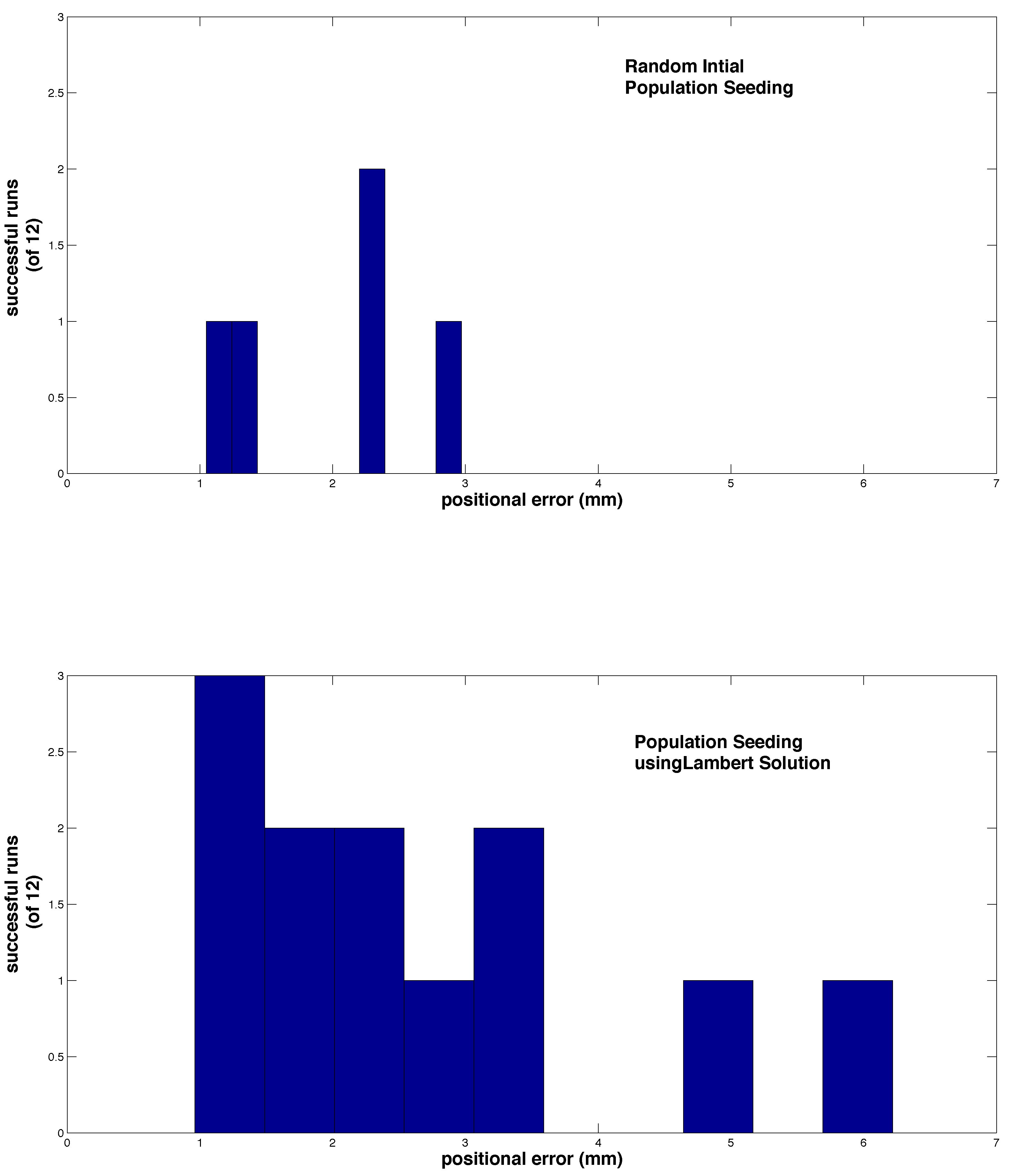
Figure 6.
Trajectories of the 11 successful runs for Problem #1. The analytical trajectory is shown in black. (left): earth scale view; (right): close up of the best solutions from DE (before fminsearch) near target .
Figure 6.
Trajectories of the 11 successful runs for Problem #1. The analytical trajectory is shown in black. (left): earth scale view; (right): close up of the best solutions from DE (before fminsearch) near target .
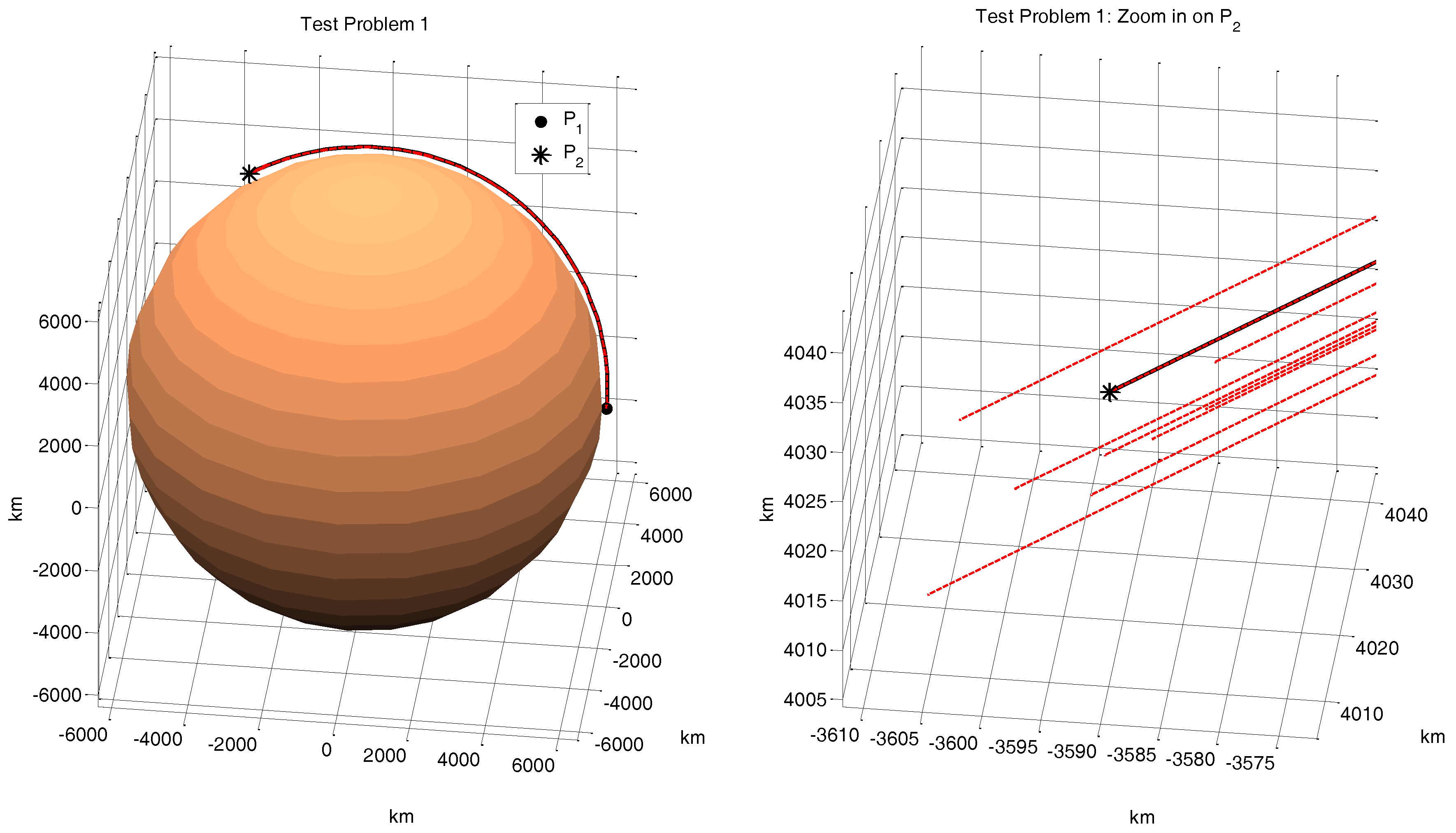
Figure 7.
Trajectories of the 11 successful runs for Problem #2. The analytical trajectory is shown in black. (left): earth scale view; (right): close up of the best solutions from DE (before fminsearch) near target .
Figure 7.
Trajectories of the 11 successful runs for Problem #2. The analytical trajectory is shown in black. (left): earth scale view; (right): close up of the best solutions from DE (before fminsearch) near target .

Figure 8.
Trajectories of the 12 successful runs for Problem #3. (left): earth scale view; (right): close up of the best solutions from DE (before fminsearch) near target .
Figure 8.
Trajectories of the 12 successful runs for Problem #3. (left): earth scale view; (right): close up of the best solutions from DE (before fminsearch) near target .

Figure 9.
Trajectory of the most successful run for Problem #4a. To avoid confusion, only the five orbits of the most successful trials are shown. (left): earth scale view; (right): close up of the best solution from DE (before fminsearch) near target .
Figure 9.
Trajectory of the most successful run for Problem #4a. To avoid confusion, only the five orbits of the most successful trials are shown. (left): earth scale view; (right): close up of the best solution from DE (before fminsearch) near target .
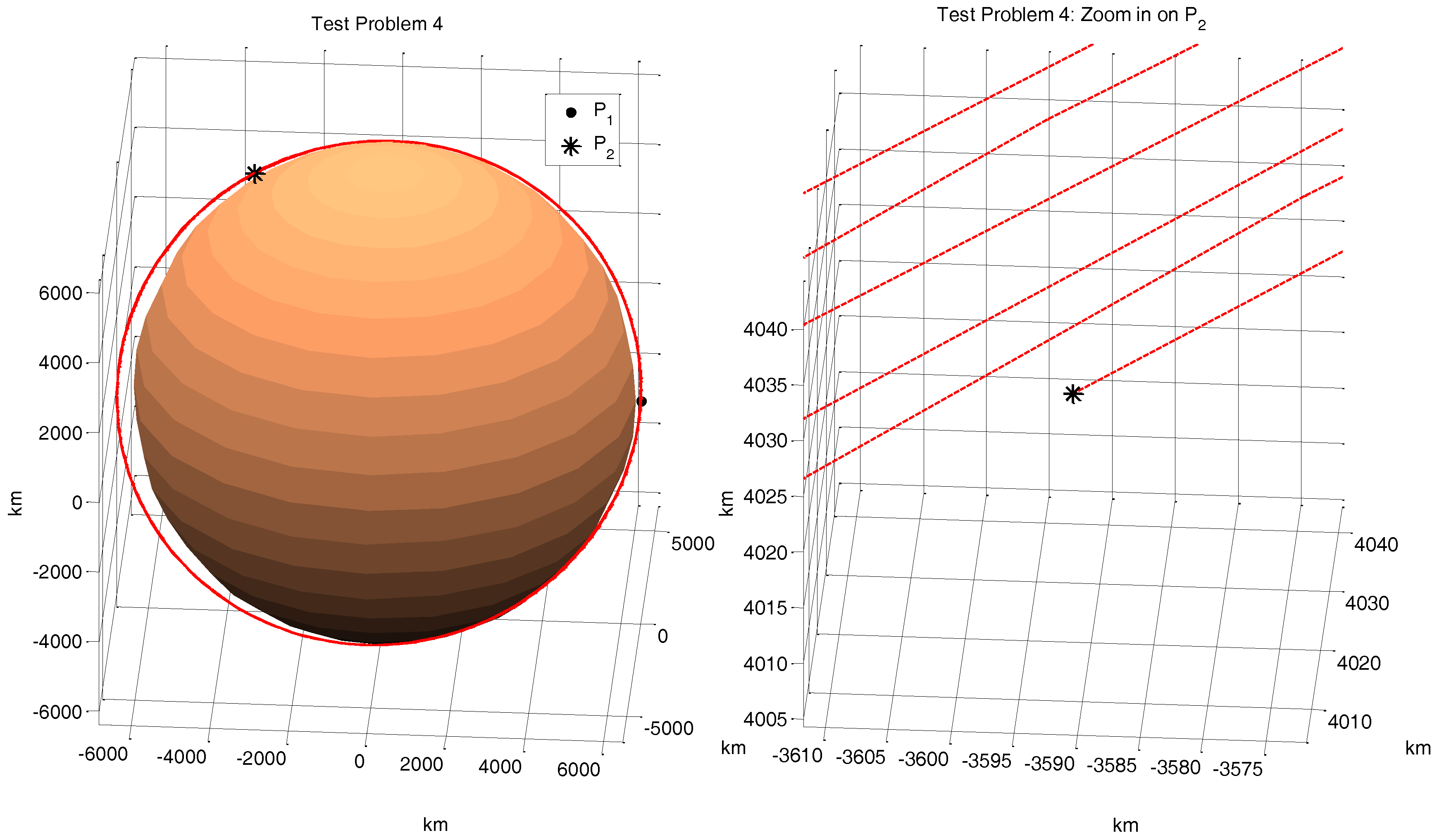
Figure 10.
Trajectory of the most successful run for Problem #4b with a 20-orbit intercept. The precession of the orbit due to the inclusion of oblateness perturbation is evident. (top) earth scale view; (bottom) close up of the best multi-orbit solution from DE (before fminsearch) near target .
Figure 10.
Trajectory of the most successful run for Problem #4b with a 20-orbit intercept. The precession of the orbit due to the inclusion of oblateness perturbation is evident. (top) earth scale view; (bottom) close up of the best multi-orbit solution from DE (before fminsearch) near target .

Table 1.
Parameter values for the Test Problems #1–4 (NA = not applicable).
| Problem | Decision Variables | (min) | |||
|---|---|---|---|---|---|
| 1 | 3 | 30 | 10 | 0 | 0 |
| 2 | 4 | NA | 1 | 25 | 0 |
| 3 | 3 | 30 | 1 | 0 | |
| 4a (5 orbits) | 3 | 479.895 | 1 | 0 | |
| 4b (20 orbits) | 3 | 1829.58 | 1 | 0 | |
| 4c (100 orbits) | 3 | 9027.90 | 1 | 0 |
Table 2.
Number of successful trials (out of 12), average positional of successful trials, positional error of best trial out of 12 for the various test cases.
Table 2.
Number of successful trials (out of 12), average positional of successful trials, positional error of best trial out of 12 for the various test cases.
| Test Problem | Successful Trials | Avg Pos Err (m) | Best Pos Err (m) |
|---|---|---|---|
| 1 | 11 | 0.023 | 9.3 |
| 2 | 11 | 0.071 | 6.7 |
| 3 | 12 | 0.003 | 9.6 |
| 4a | 12 | 2.66 | 9.63 |
| 4b (20 min) | 5 | 3.04 | 1.12 |
| 4b (60 min) | 7 | 1.17 | 9.43 |
| 4c (60 min) | 0 | 104200.7 | 3.40 |
| 4c (120 min) | 4 | 81424.7 | 1.16 |
© 2017 by the authors. Licensee MDPI, Basel, Switzerland. This article is an open access article distributed under the terms and conditions of the Creative Commons Attribution (CC BY) license (http://creativecommons.org/licenses/by/4.0/).
Share and Cite
MDPI and ACS Style
Hinckley, D.W., Jr.; Hitt, D.L. Evolutionary Approach to Lambert’s Problem for Non-Keplerian Spacecraft Trajectories. Aerospace 2017, 4, 47. https://doi.org/10.3390/aerospace4030047
AMA Style
Hinckley DW Jr., Hitt DL. Evolutionary Approach to Lambert’s Problem for Non-Keplerian Spacecraft Trajectories. Aerospace. 2017; 4(3):47. https://doi.org/10.3390/aerospace4030047
Chicago/Turabian StyleHinckley, David W., Jr., and Darren L. Hitt. 2017. "Evolutionary Approach to Lambert’s Problem for Non-Keplerian Spacecraft Trajectories" Aerospace 4, no. 3: 47. https://doi.org/10.3390/aerospace4030047
Note that from the first issue of 2016, this journal uses article numbers instead of page numbers. See further details here.