Queue-Based Modeling of the Aircraft Arrival Process at a Single Airport


1
Air Traffic Management Department, Electronic Navigation Research Institute, National Institute of Maritime, Port and Aviation Technology, Tokyo 182-0012, Japan
2
Faculty of Aerospace Engineering, Delft University of Technology, HS 2926 Delft, The Netherlands
*
Author to whom correspondence should be addressed.
Aerospace 2019, 6(10), 103; https://doi.org/10.3390/aerospace6100103
Submission received: 19 August 2019
/
Revised: 9 September 2019
/
Accepted: 16 September 2019
/
Published: 20 September 2019
(This article belongs to the Collection Air Transportation—Operations and Management)
Abstract
:This paper proposes data-driven queuing models and solutions to reduce arrival time delays originating from aircraft arrival processing bottlenecks at Tokyo International Airport. A data-driven analysis was conducted using two years of radar tracks and flight plans from 2016 and 2017. This analysis helps not only to understand the bottlenecks and operational strategies of air traffic controllers, but also to develop mathematical models to predict arrival delays resulting from increased, future aircraft traffic. The queue-based modeling approach suggests that one potential solution is to expand the realization of time-based operations, efficiently shifting from traffic flow control to time-based arrival management. Furthermore, the proposed approach estimates the most effective range of transition points, which is a key requirement for designing extended arrival management systems while offering automation support to air traffic controllers.
1. Introduction
Global air traffic passenger demand is expected to increase 250% in the next 20 years [1]. To accommodate such air traffic growth, the air traffic management system strives to provide the airports and the sectors the traffic capacities needed to ensure arrival traffic punctuality, while having ecologically and economically friendly flights. At the same time, high levels of air traffic safety must be maintained. Reducing arrival delays is one of the most important functions of a ground arrival management (AMAN) system, which provides air traffic controllers with automation support for sequencing and spacing.
AMAN design requirements depend on the characteristics of a given arrival air traffic flow and its surrounding environment, e.g., runway and airspace capacity, weather conditions, air routes, and other geographical constraints. In the United States, the Traffic Management Advisory [2] was deployed in air traffic control centers in the 1990s, while its enhanced versions, the Time-Based Flow Management [3] and Terminal Sequencing and Spacing [4], take into account future airborne-based operations [5]. These systems contribute to consistency in sequencing and time-spacing of arrival traffic in en-route and terminal airspace areas. In Europe, the ongoing SESAR project has facilitated collaboration among European countries and contributed to the development of “Enhanced” AMAN, which coordinates arrival time-schedules covering wider ranges of airspace than in the case of conventional operations [6]. Focusing on the busy terminal area, metaheuristics active solutions for efficient aircraft scheduling and re-routing were proposed to enable real-time optimization within a small computation time [7]. In the Asia-Pacific strategic air traffic flow management region, the Long Range Air Traffic Flow Management has been devised to provide a basis for research into applications beyond current system time-frames [8]. Ongoing Japanese research and development on “Extended” AMAN (E-AMAN) aims to achieve efficient arrival traffic flow at Tokyo International Airport [9]. To analyze bottlenecks that future arrival traffic flow may bring, mathematical models are useful to predict causes and provide solutions for reducing arrival delay times. In this light, we apply queue-based modeling for arrivals at a single airport and discuss new procedures and technologies that support air traffic controllers in handling arrival traffic at congested airports. Our proposed queuing approach provides closed-form analytical results about flight delay bottlenecks in the airspace area around the airport.
Several studies have modeled aircraft arrival and departure operations using queuing-based models. Air traffic in a sector is modeled in [10] as an M/M/s queue where the sector capacity s is defined as the number of aircraft transiting this sector at any time. This M/M/s queue is coupled to an M/M/1 queue that generates communication messages to be handled by air traffic controllers. Modi [10] established relations between the rate of communication messages for air traffic controllers and the aircraft arrival rate in the sector. A network of queues is employed to model a system of multiple airports in [11,12]. In [11], the propagation of delays is analyzed in a system of airports by means of queues. In [12], a Jacksonian network with queues is used to model the entirety of air traffic over US airspace. The results show that this modeling approach approximates well a Monte Carlo simulation of the same system. Aircraft departures at a single airport are analyzed in [13] by means of a queuing model. With the runway schedule as input, the model outputs the expected runway waiting time for an aircraft prior to departure. This model was applied in a case study for Newark Liberty International Airport to predict taxi-out times. In [14], a queuing model is used to estimate the taxi-out time at Boston’s Logan Airport. The arrival process at an airport is analyzed in [15,16], with particular focus on runway-related delays. In [15], the expected waiting time for aircraft arriving on a single runway is determined using an queuing model. Simple bounds for the expected waiting time are determined by comparison to the and models. However, the authors did not make use in their case study of operational data or compare their results against actual data. In [16], the US National Airspace System is modeled as a network of queues, with the TRACON sectors being modeled as an queue. All the above models assume that arrivals and/or service times follow exponential or Erlang distributions. However, when analyzing actual air traffic data, these assumptions do not hold. In fact, it is often difficult to fit traffic data on known distributions. In addition, these models assume that operations, e.g., arrivals at a runway, occur one by one. Thus, the authors often make use of single-server queuing models. However, when considering the time aircraft use (fly within) airspace, several aircraft can be flown at the same time in an airspace. To model this, we assume a multi-server queue. As such, we consider a queuing model that characterizes better the actual traffic data.
Given the above, the present paper proposes a queue-based modeling approach to estimating flight arrival delays and the impact of decreasing flight separation in the context of E-AMAN. We applied our models to arrival traffic at Tokyo International Airport, which is the world’s fifth busiest airport with respect to passenger traffic. Our analysis builds on a data-driven analysis of actual flight plans and arrival flight track data. The contribution of this paper is twofold. First, we propose an analytical approach for estimating aircraft time delays in an extended area around a destination airport, while taking into account current aircraft separation and airspace capacity restrictions. Second, we analyze the impact on aircraft delays when considering novel arrival procedures that can accommodate increased arrival traffic volumes by reducing the minimum aircraft separation.
This paper is organized as follows. Section 2 introduces air traffic operations at Tokyo International Airport, and characterizes the arrival traffic data recorded in 2016 and 2017. This data analysis supports the models subsequently presented. Section 3 proposes a queue-based modeling approach in which the aircraft arrival process is formulated as a queuing model. Based on the data-driven analysis, probability distributions of the inter-arrival time and service time are estimated. In Section 4, the queuing model is applied in estimating aircraft arrival delay time as a function of the distance from the airport. The estimation results permit analysis of the relationship between arrival rate and aircraft waiting time. In Section 5, we analyze the positive impact on the airspace capacity of reducing inter-arrival time within the arrival traffic flow. In this context, aircraft delay time is estimated by means of the proposed queue-based approach. Section 6 discusses how this proposed queue-based approach contributes to the design of E-AMAN procedures and technologies. Additionally, our future work on the mathematical modeling of the aircraft arrival process is discussed, as are further extensions of the study. Finally, Section 7 provides conclusions and outlines our plans for future work.
2. Case Study Data Description—Tokyo International Airport
2.1. Runway Layout
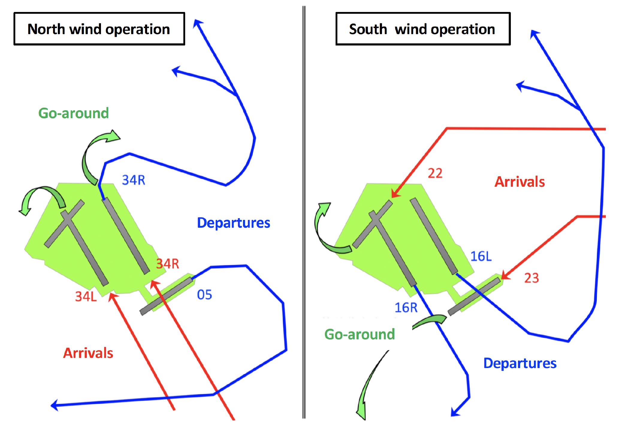
Tokyo International Airport is the fifth busiest airport in the world with respect to passenger traffic, with a total of 83,189,933 passengers in 2017. An increase of % in the number of passengers was registered in 2017 relative to 2016 [17]. An overall maximum of 447,000 flights (departures and arrivals) are accepted per year, with a maximum of 80 operations each hour. Over of the domestic flights in Japan are concentrated at this airport. The airport makes use of four runways on a daily basis, while the choice of the runway configuration depends on the wind direction (see Figure 1). In north wind operations, runway 34L is used for arrivals from the southwest, runway 34R being used for arrivals from the north as well as for departure traffic. In south wind operations, runway 22 is used for arrivals from the southwest, and runway 23 for arrivals from the north.
2.2. Statistical Analysis of the Arrival Air Traffic Flow
The present case study was based on flight plans and track data for a period of 71 days selected from the odd months of 2016 and 2017. All data cover nominal operation at Tokyo International Airport excluding weather impacts and other rare events. In 2016, there were, on average, 608 arrivals per day; 530 domestic and 78 international. In 2017, an average of six more international flights were accepted each day compared to 2016. Thus, 2017 saw a total of 614 arrivals per day; 530 domestic and 84 international.
Table 1 shows the types of aircraft, by percentage, used for arrivals and departures. The majority of the aircraft are used for short- and medium-distance passenger transportation: A737-800 (B738), A320, and B767-300 (B763). Long-distance passenger aircraft such as B777-200 (B772) and B787-8 (B788) are also used. Fewer than of the flights are business jets, such as the Gulfstream and Bombardier aircraft.
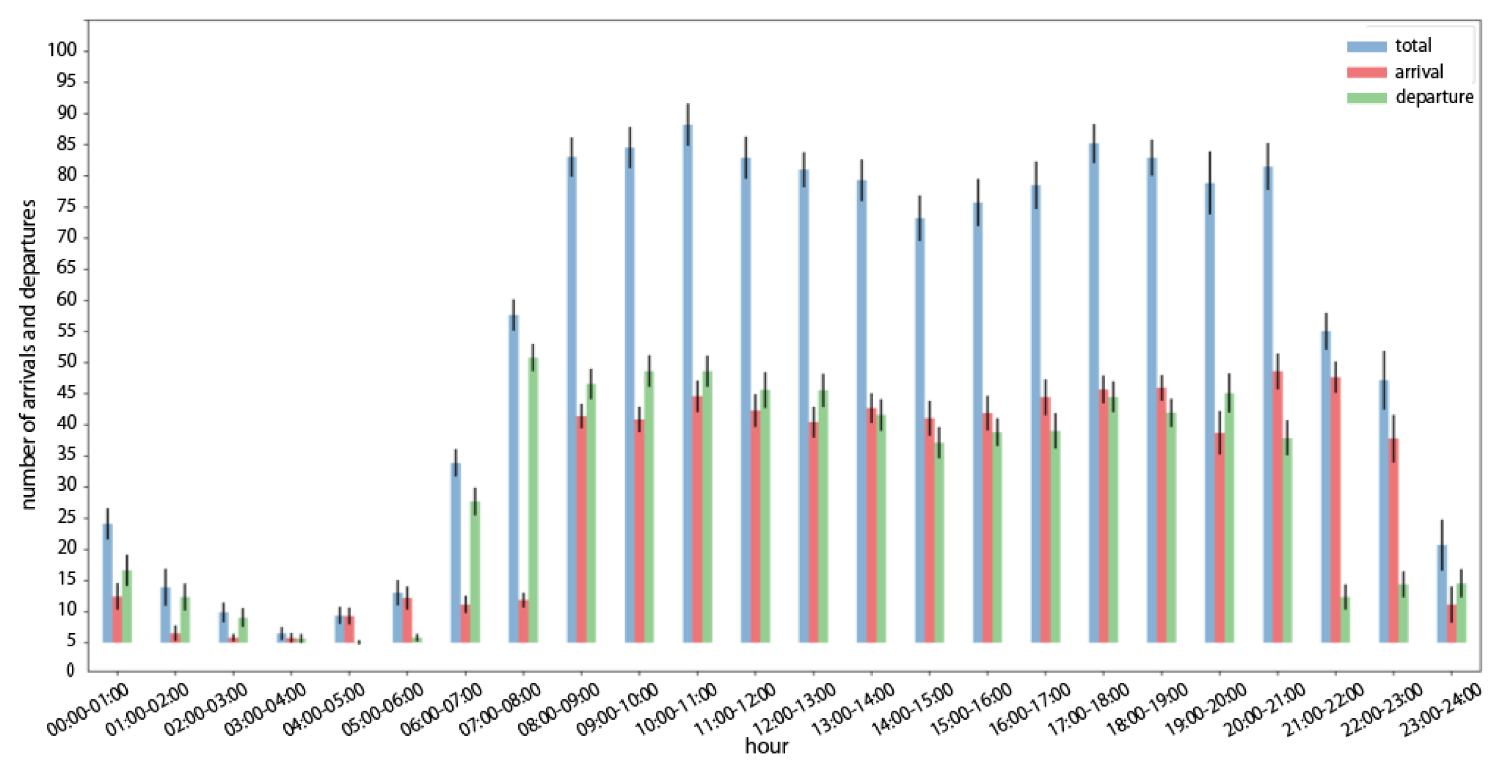
Figure 2 shows the mean of flight arrivals and departures for each hour of the day. The black whisker shows the standard deviation of the number of arrivals and departures in an hour. The total number of arrivals between 08:00 and 23:00 is slightly below the maximum allowed daily traffic thresholds, with the most congested period occurring between 17:00 and 22:00.
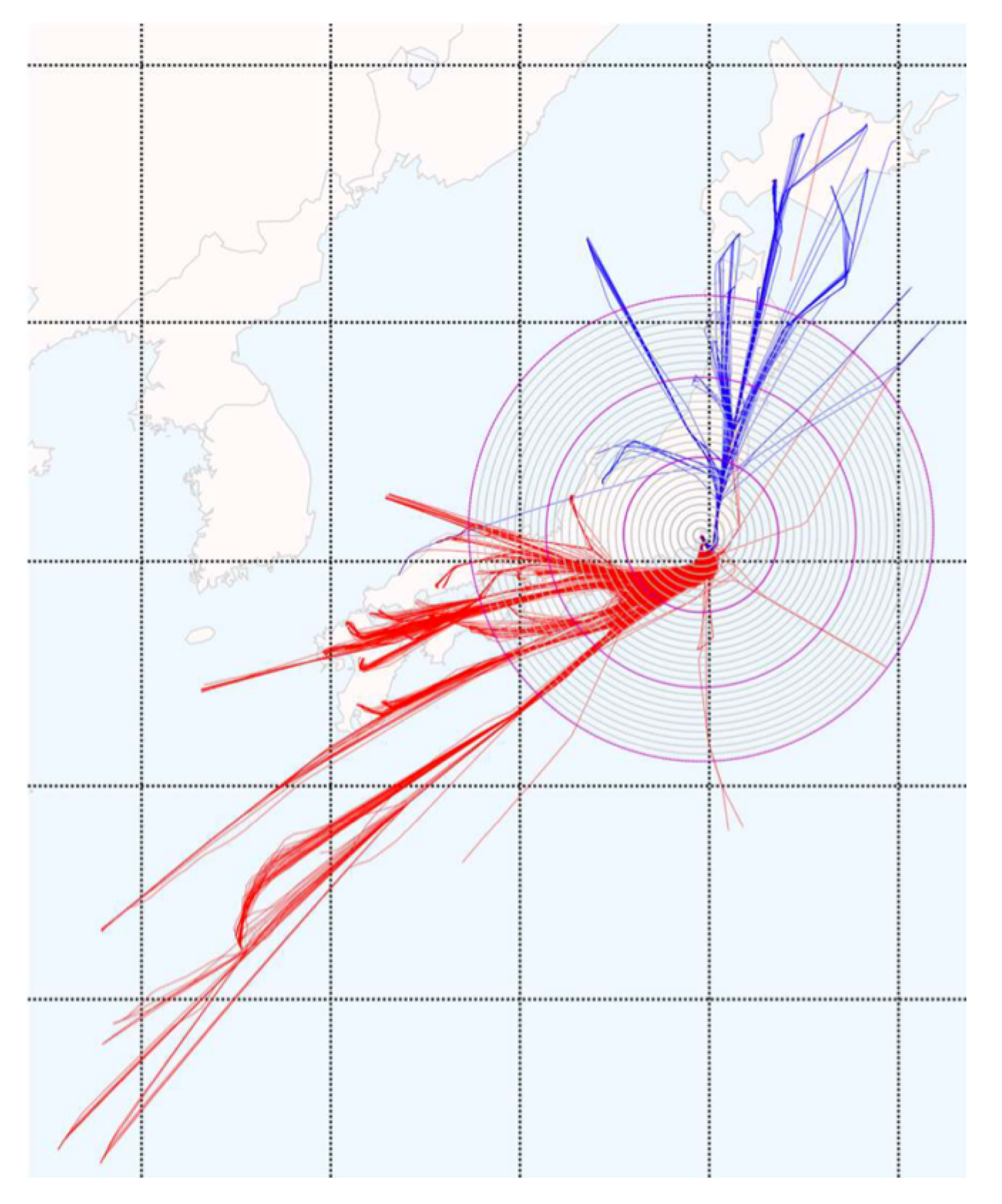
One salient feature of arrival traffic flow at Tokyo International Airport is that the arrivals come in either from the north or from the southwest. In the period from 08:00 to 23:00, an average of 569 arrival flights; 422 from southwest and 147 from the north. Figure 3 shows the flight track data for one day of operations in November 2016. The flight tracks of the arrivals using runway 34L are shown in red, while the flight tracks of the arrivals using runway 34R are shown in blue. Concentric circles, centered at Tokyo International Airport, are shown for radii at increment of ten nautical miles (NM), from 10 to 300 NM.
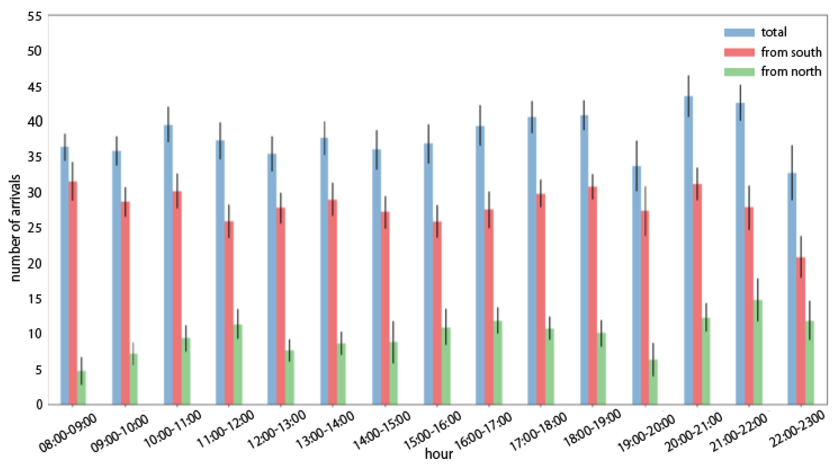
Figure 4 shows the hourly number of flights arriving from southwest and from the north each hour between 08:00 and 23:00. The number of arrivals from southwest is approximately three times that from the north. In the near future, the number of arrivals from southwest is expected to grow as a result of an increasing Asian traffic demand [1].
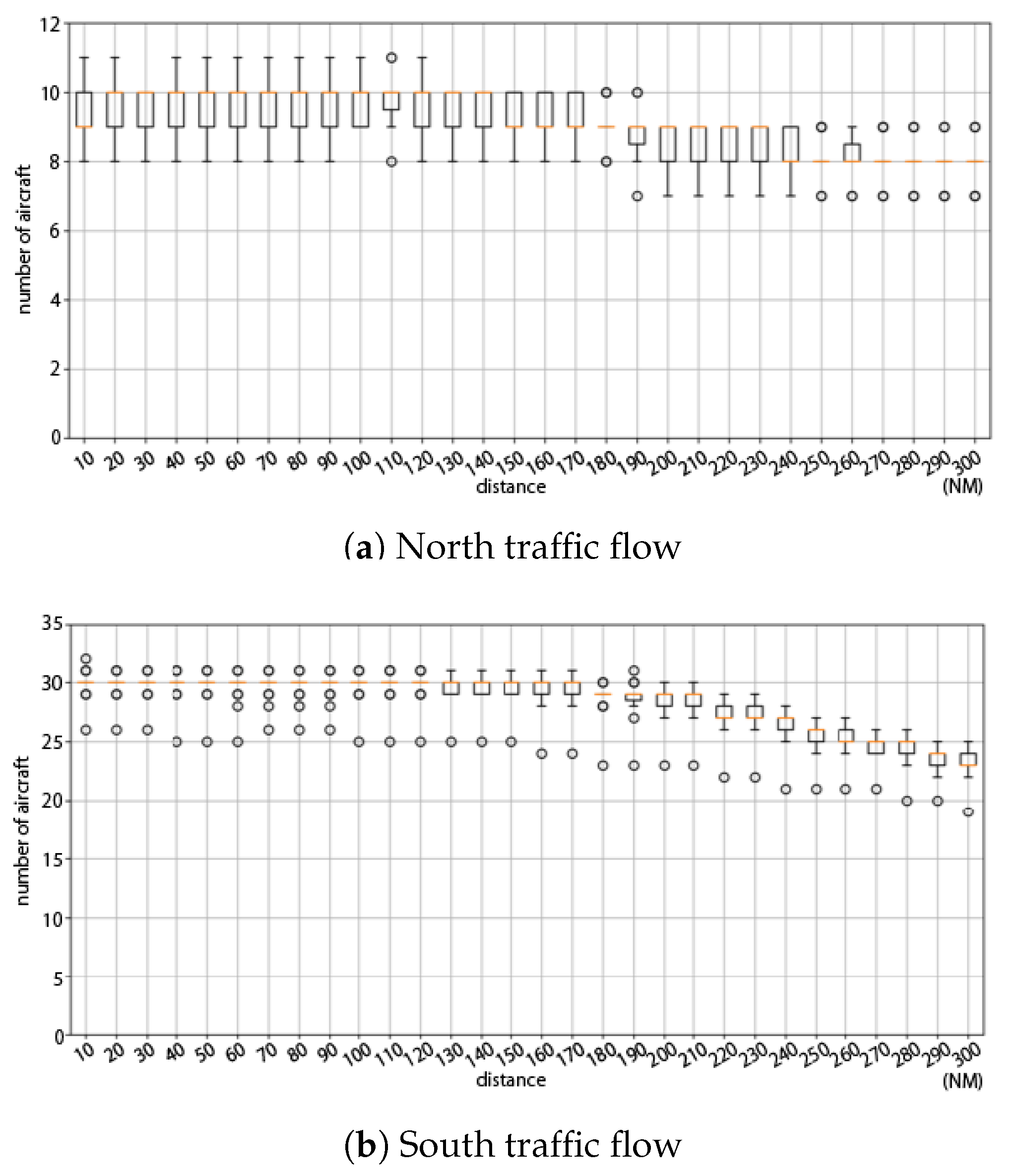
Air traffic flow in Japan is controlled, with a central focus on arrivals at Tokyo International Airport. Figure 5 shows the average number of arrival flights crossing every concentric circle (see also Figure 3) each hour between 17:00 and 22:00 for all the days. The total number of arrivals is kept to a maximum 40, including 30 from southwest and 10 from the north.
3. Model Description and Formulation of the Aircraft Arrival Traffic
3.1. Model Description and Formulation of the Aircraft Arrival Process as a Queuing Model
Given the statistical analysis in Section 2, we propose a queuing model for arrival traffic from the southwest arriving at Tokyo International Airport between 17:00 and 22:00, which represents the most congested arrival period at Tokyo International Airport.
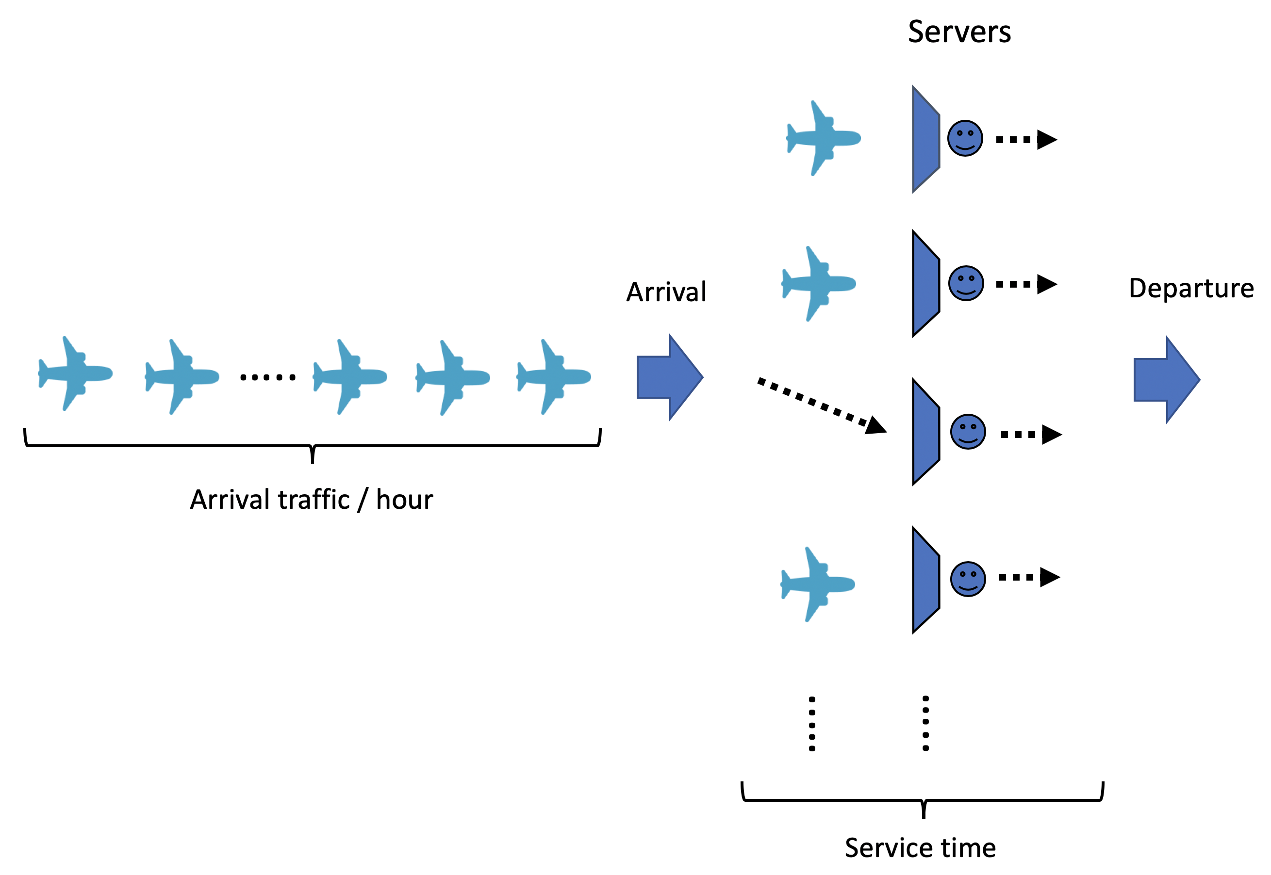
We specify our queuing model using an arrival flow, a service time, and a number of servers (see Figure 6) as follows. The aircraft arrive at a given airspace according to an hourly rate, i.e., a set number of arrivals per hour. The arrivals are separated in time for safety reasons. The time between two consecutive arrivals at an airspace is called the aircraft inter-arrival time. Upon arrival, the aircraft receive a service time, i.e., the time the aircraft spends flying the given airspace. We consider a multi-server queuing model, in which the number of servers indicates the number of aircraft that are allowed to be present at any time in the given airspace, i.e., the capacity of the given airspace.
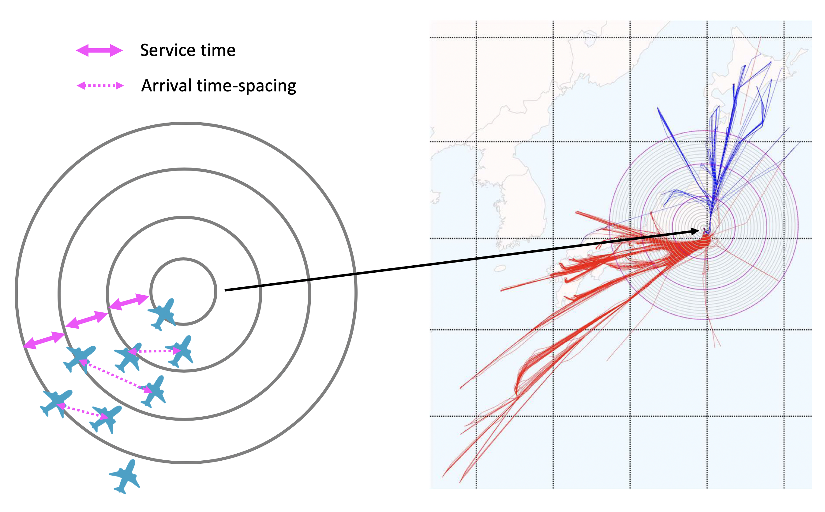
We formulate this aircraft arrival process by means of a queuing model as follows. We consider an airspace area of radius 300 NM around the airport. We partition this area using concentric circles (see Figure 7) centered at the airport, with radii at increments of 10 NM. This partitioning defines 29 airspace areas , where area 1 is the airspace area around the airport in the circular ring defined by the 10 and 20 NM radii, area 2 is the airspace area around the airport in the circular ring defined by the 20 and 30 NM radii, and so on. An aircraft traffic flow arriving at area 1 crosses the circle of radius 20 NM, while an aircraft arriving at area 2 crosses the circle of radius 30 NM, and so on. By analyzing the historical traffic data, the arrival and service times could not be fitted to specific distributions such as exponential or normal distribution. Thus, we assumed general, data-based distributions to characterize the arrival process of aircraft at an airspace and the time to fly in a given airspace. In addition, to model the fact that several aircraft can be present at the same time in a given airspace, we assumed a multi-server queue.
We analyze each specific airspace independently. We are interested in the delays associated with arrivals in a specific area defined by two concentric circles, with a radius difference of 10 NM. This analysis based on an airspace defined by concentric circles can support the design of new sectors around the Tokyo International Airport, which is currently an on-going process at this airport.
3.2. Data-Driven Analysis of the Flight Arrival Traffic
Our modeling approach in Section 3.1 is motivated by a data-driven analysis based on the flight plans and radar data corresponding to the arrival aircraft in 2016 and 2017. Figure 8 shows the empirical distribution of service times corresponding to the airspace area with Gaussian fitting. As shown in Figure 8, a Gaussian distribution approximates well the service time distribution.
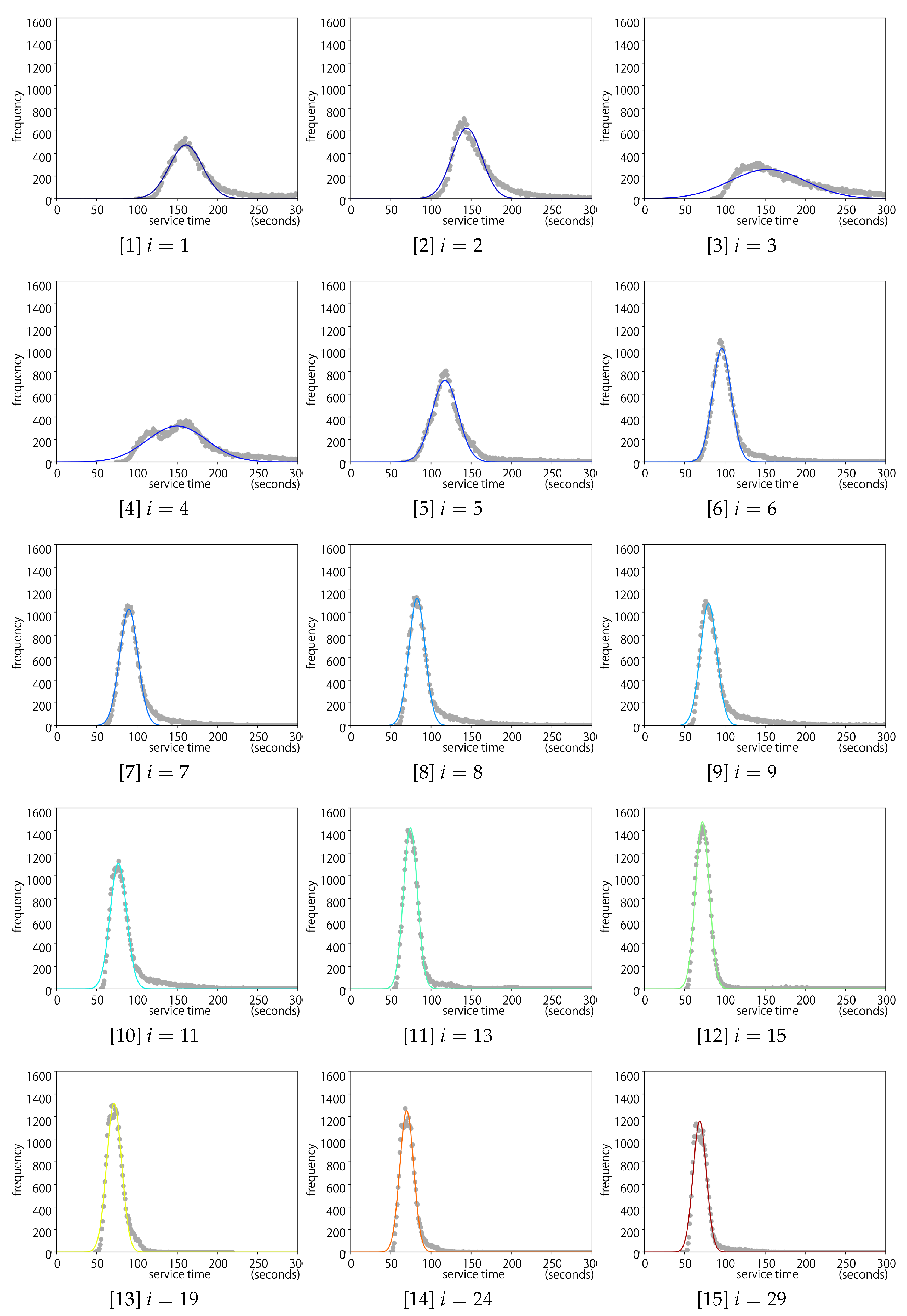
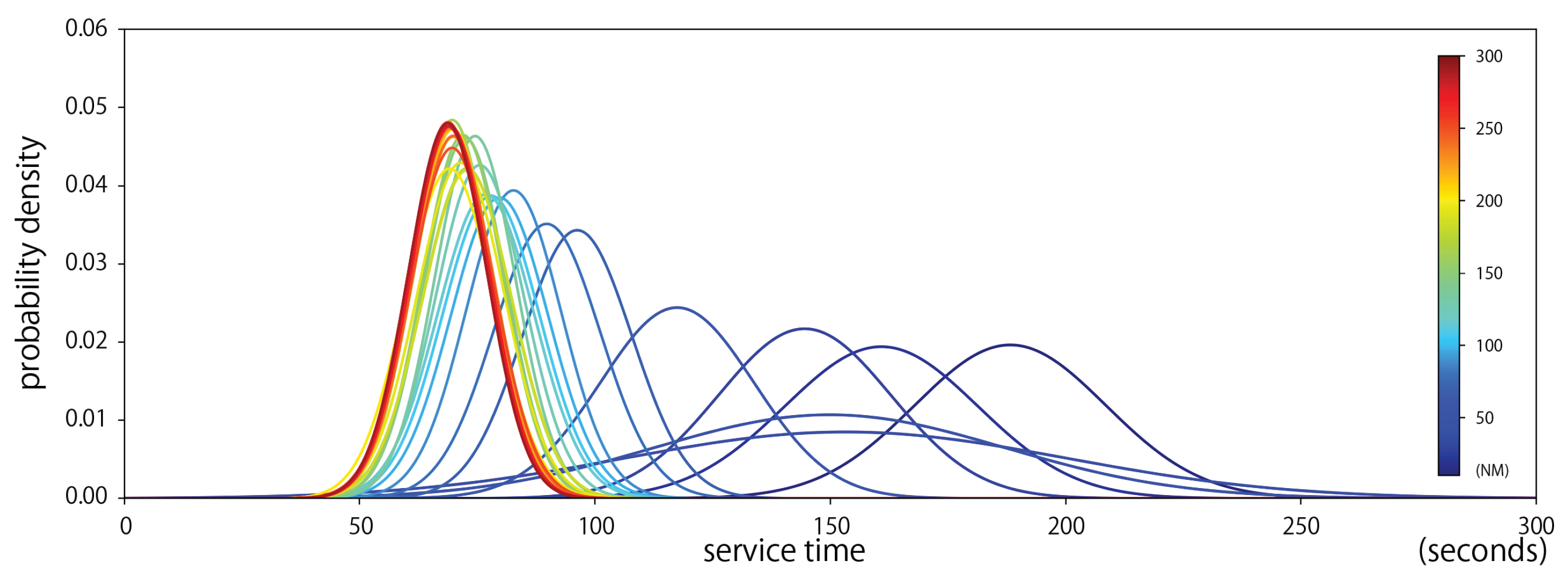
Figure 9 shows the characteristics of the empirical service time distribution corresponding to airspace area and Gaussian fitted distributions. Comparing these probability densities clarifies not only the empirical distributions of the service time in the assigned airspace, but also emphasizes the current strategies that the air traffic controllers use for arrivals at Tokyo International Airport. One of the most significant strategies is illustrated in the service time distribution for the airspace areas and , which, together, correspond to the airspace between the concentric circles of radii 30 and 50 NM. Figure 9 shows that the service time variance is enhanced in these airspace areas compared to other areas. This is explained by the fact that the arrival time-spacing is actively conducted by air traffic controllers in the airspace between concentric circles of radii 30 and 50 NM, just before the aircraft enter the terminal area. The increase in both the mean service time and the service time variance in the direction of the airport is due to the airspeed reduction that arriving aircraft undertake prior to landing. For service time, the mean and variance converge close to the circle of radius 200 NM. This circle captures current arrival strategies, since this is the airspace within which the traffic control capacity is met and the spacing at merging points is filled. Between circles of radii 200 NM and 300 NM, air traffic controllers make an effort to maintain safe and efficient traffic flows by prioritizing airlines’ own procedures. In summary, there are three main strategies illustrated by the service time distributions for arriving aircraft: (i) arrival time-spacing within the circle around 50 NM, especially between the 30 and 40 NM radii circles; (ii) arrival metering for traffic capacity control and spacing at merging points between the 50 and 200 NM circles; and (iii) maintaining efficient traffic flow by prioritizing airlines’ own procedures beyond the 200 NM circle. Minimizing arrival delays and operational costs requires great consideration in combining these different strategies.
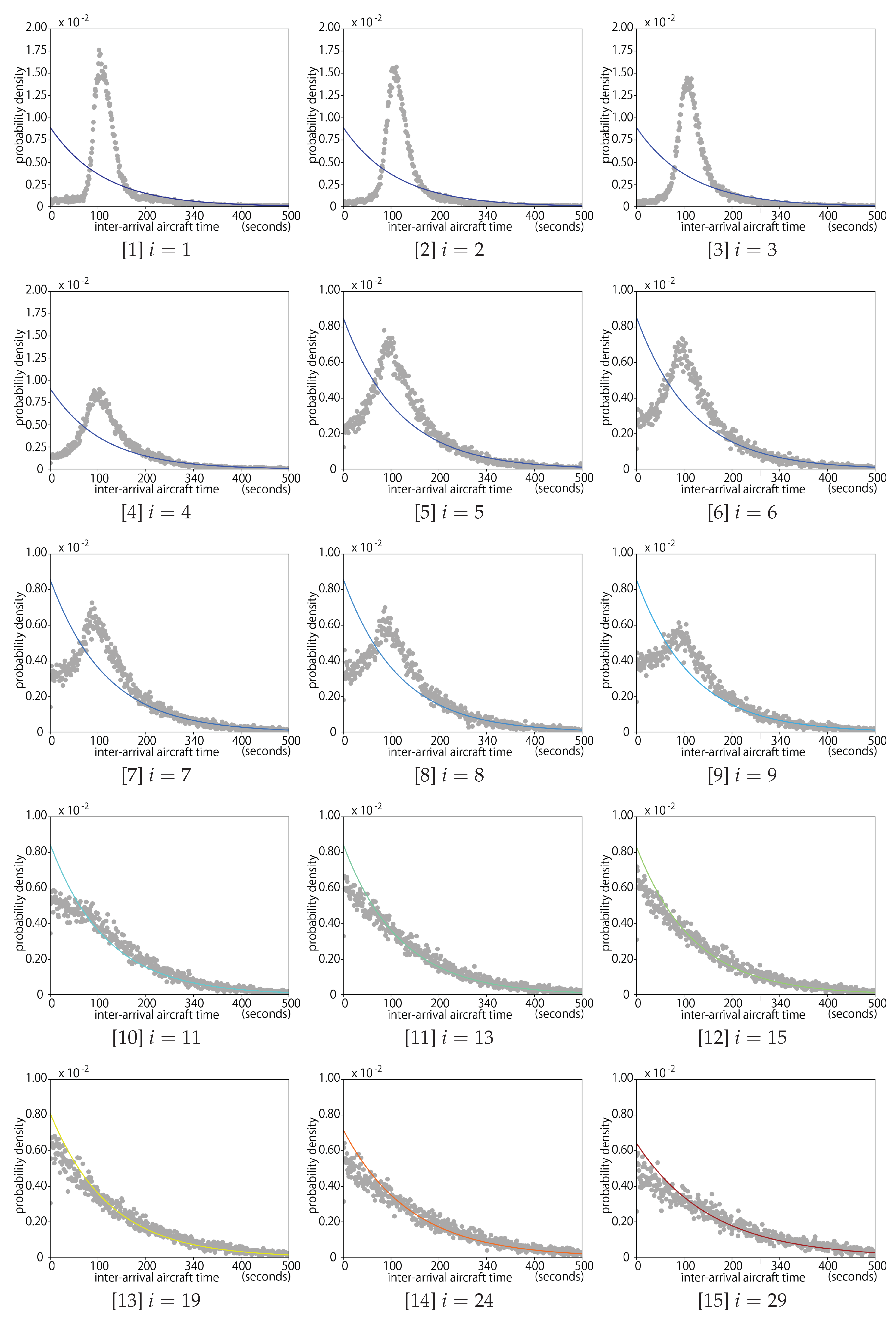
Figure 10 compares empirical probability densities of aircraft inter-arrival time corresponding to airspace area with their exponential fittings. Figure 10 shows that the empirical distribution of the inter-arrival time is well approximated by an exponential distribution where the arriving aircraft fly beyond the 150 NM circle. However, the inter-arrival times converge to a nearly Gaussian distribution towards the departure airports. In Table 2, is the empirical coefficient of variance defined as:
where and are, respectively, the mean inter-arrival time and the variance of the inter-arrival time in airspace i. When , the empirical distribution of the inter-arrival time is well approximated by an exponential distribution. For values much larger or smaller than 1, the empirical distribution deviates from exponential.
Based on the results of the data analysis above, we model the aircraft arrival process in an airspace area using a model, where both service time and inter-arrival time follows general distributions. Aircraft arrive at area according to a general probability distribution specific to that region. Upon arrival at airspace area i, aircraft spend a random amount of time flying in this airspace before arriving at airspace . The flying time for an aircraft in an airspace area follows a general probability distribution specific to that region. In each airspace area, aircraft with the same number of servers c are at most allowed to be present at the same time. This constraint reflects the capacity constraints imposed on the aircraft arrival airspace. As a result, additional aircraft need to delay their entrance mainly by means of vectoring and/or speed adjustments. We define aircraft processing time in region i as the flying time in airspace area i plus any delay imposed in airspace area i due to congestion in area .
We model the aircraft present in an airspace area as a queue. The inter-arrival times in airspace area are identically and independently distributed according to a general distribution with finite mean. Let denote the expected inter-arrival time of aircraft arriving in airspace area . The aircraft service times are independent and identically distributed according to a general distribution with finite mean. Let denote the expected service time of aircraft in airspace area , i.e., an aircraft’s expected flying time in area i. Aircraft inter-arrival times and service times are independent of each other. Let denote the mean amount of work that arrives per unit time in airspace area . In addition, there are c parallel, identical servers. To ensure queue stability, we have that:
Equation (2) ensures that the rate at which aircraft arrive at airspace area is lower than the rate at which aircraft are serviced in this area and, consequently, the aircraft queue length remains finite in the long -run. Table 2 shows the values of for , all parameters in Equations (1) and (2), and corresponding to data between 17:00 and 22:00. As shown in Table 2, is satisfied for all i.
4. Analyzing Aircraft Arrivals Using a G/G/c Queuing Model
4.1. Determining Aircraft Delay Time
In this section, we determine the time an aircraft is potentially delayed during the flight. Here, an airborne delay is achieved by requesting the aircraft to fly a longer route, i.e., vectoring/metering/speed adjustments.
Let denote the delay that an aircraft experiences in the airspace area due to lack of capacity in the area . Following the authors of [18,19,20,21], we approximate the total airborne delay in airspace area i as follows:
where is the squared coefficient of variation of the aircraft inter-arrival time in airspace area i and is the squared coefficient of variation of the aircraft service time in airspace area i.
In Equation (3), denotes the expected aircraft delay time in airspace area i when a queuing model is considered. This means that the arrival process is considered a Poisson process with a parameter , where service times are assumed to follow an exponential distribution with a parameter and there is a fixed number of parallel servers c. Moreover, for stability, we have that .
The expected delay in an queuing model with Poison arrivals with rate , mean exponential service time and c parallel, identical servers is well-known and determined, following [22,23]. Let denote the probability of having n customers in the system. The balance equations of an queuing model are then:
Recursively solving Equation (4), . Now, using that , it follows that
Finally,
We also note from Equation (4) that . With as the probability that an arriving customer in the system is delayed because there are already c or more customers in the system, and using that and Equation (6), the expected queue length, denoted by , is:
Following Little’s Law [24], we also have that
Equation (3) now follows by modeling aircraft arrivals in each area i as a queue with Poisson arrivals.
4.2. Arrival Delay Times for Different Aircraft Arrival Rates
In this section, we determine the aircraft arrival delay in an airspace area i for the most congested time period of arrivals between 17:00 and 22:00.
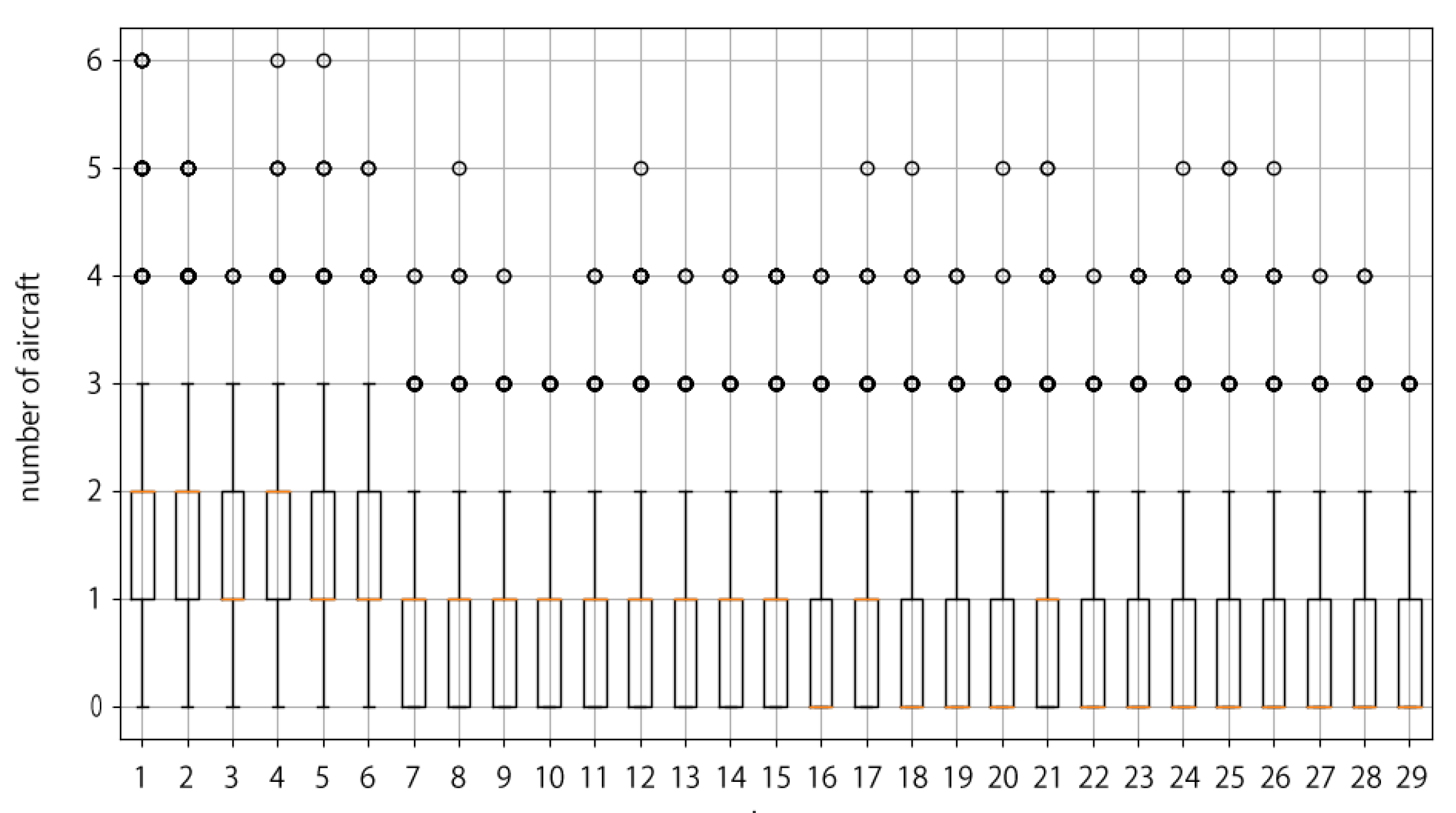
Figure 11 shows the number of aircraft flying in airspace area . We consider to represent the current airspace capacity since the data show the highest mean number of aircraft in an airspace to be at most two across all considered airspace i. As shown in Figure 11, the median in the terminal area approximately within 50 NM, where , takes 2 () or 1 (), and the median in the en-routes takes 1 or 0. The mean at is larger than 1. The reason to give the value for airspace is also relevant from the perspective of safety in air traffic control in the en-route airspace. In particular, the inter-arrival aircraft distance is approximately 5 NM (i.e., two aircraft within a 10 NM range), which is exactly the minimum aircraft separation currently needed for radar separation in the en-route airspace.
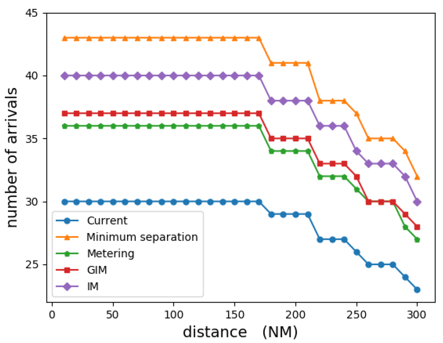
As shown in Figure 5b, the maximum volume of arrivals from the southwest direction is 30 aircraft per hour. This number can be adjusted to account for increased runway throughput. One potential way to increase the number of arrivals per hour is to apply new wake vortex categories, so-called RECAT (Wake Turbulence Re-categorisation), which enable shorter inter-arrival aircraft times than the current operation at Tokyo International Airport.This paper considers a new wake vortex category, which is currently under review in ICAO’s Wake Turbulence Working Group.
Figure 12 compares current and estimated, future volumes of arrival traffic. The estimated arrival traffic volumes are determined by applying the Wake Turbulence Re-categorization (RECAT), which is “minimum separation” for three automation levels: “Metering”, “GIM (Ground-based Interval Management)”, and “IM (Interval Management)” [25]. “Metering” operations constitute ATCo’s sequencing and spacing tasks currently supported by AMAN. “GIM” operations implement advanced AMAN support for ATCo. “IM” operations allow high-levels of automation support, typically a mixture of airborne self-separation and advanced AMAN usage. Each automation level affects the safety margin, which adds extra time-separation to RECAT time-separation, . As a consequence, inter-arrival time is calculated as follows:
where for “Metering”, for “GIM” and for “IM”, with hourly arrival traffic volume estimated using Equation (9), as shown in Figure 12. We use the value and the estimated aircraft delay based on Equation (3). As explained in Section 3.1, Equation (2) should be satisfied to ensure the queue stability in the model. As such, we compare the current aircraft delay time (30 arrivals per hour) and Metering operation (36 arrivals per hour), which satisfy this stability condition.
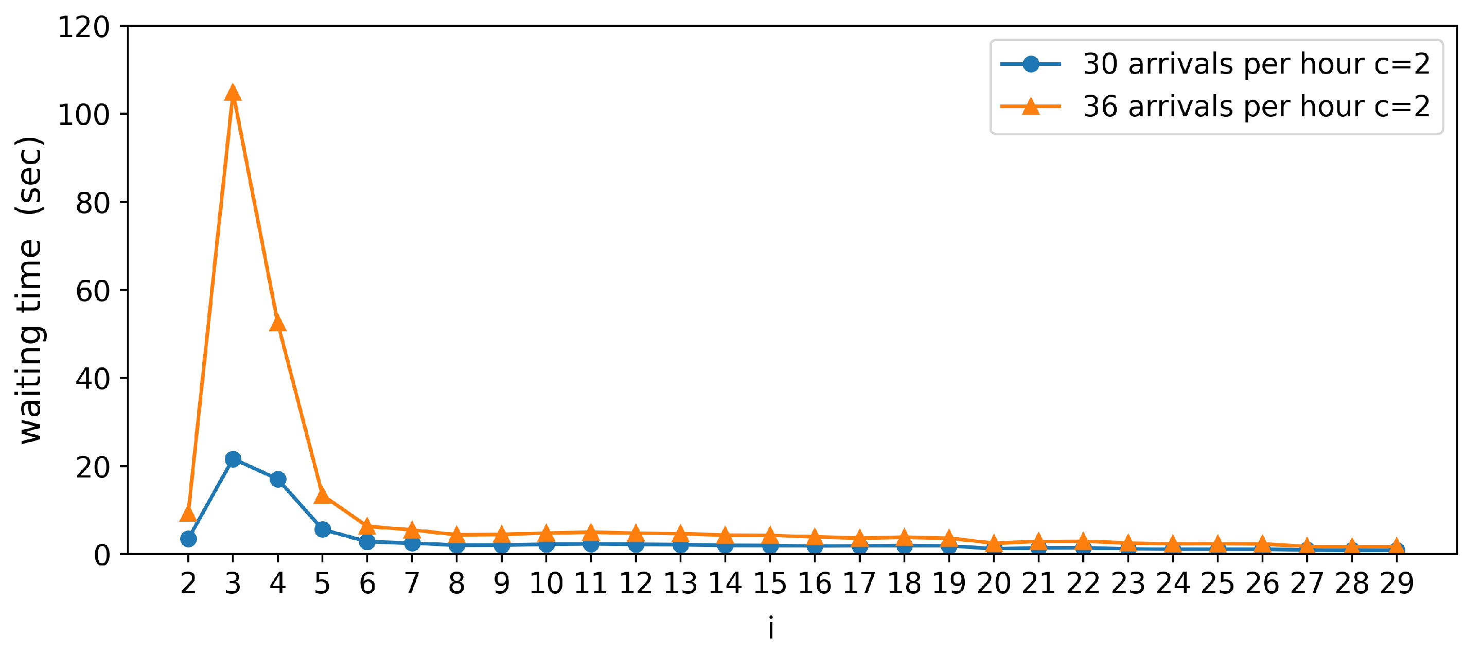
Figure 13 and Table 3 and Table 4 show the arrival delay time estimated using the model. As shown in Table 3 and Table 4, , noting that for in Table 4. Therefore, estimation results for are compared in Figure 13. In the current operations (30 arrivals per hour), the arrival delay increases by and s, respectively, in airspace area (i.e., between the circles of radii 30 NM and 40 NM) and airspace area (i.e., between the circles of radii 40 and 50 NM). When the traffic volume is increased by applying minimum separation under Metering operations (36 arrivals per hour), the arrival delay time increases to and s, respectively, in airspace and . A significant aircraft delay increase is projected in the airspace between the circles of radii 30 and 50 NM radius if the current service levels are maintained under future increases in arrival traffic volume. As shown in Figure 9 and Table 2, the variance of the service time increases in this airspace because arrival time-spacing is controlled there under current operations. If the arrival rate is increased beyond the service rate, the queue stability no longer holds in the airspace when the limiting value of aircraft is reached in each airspace.
5. Analyzing the Impact of Increased Airspace Capacity by Decreasing Minimum Aircraft Separation
In this section, we analyze the impact of increased airspace capacity using the model. Considering allows that three aircraft are served (i.e., allowed to be present) at the same time in a single airspace. As explained in Section 4.2, represents the situation where two aircraft co-occupy the assigned airspace, keeping a 5 NM minimum separation distance while flying in an airspace of 10 NM length. If is allowed in the same operation, the arrival aircraft separation can be reduced to less than 5 NM, e.g, two arrival pairs maintain a 3 NM separation while one pair maintains a 4 NM separation. Applying RECAT for current arrival sequencing with current aircraft types at Tokyo International Airport theoretically enables us to realize airspace capacity if accurate time-spacing is achieved. To increase the airspace capacity, arrival time-separation needs to be controlled more precisely.
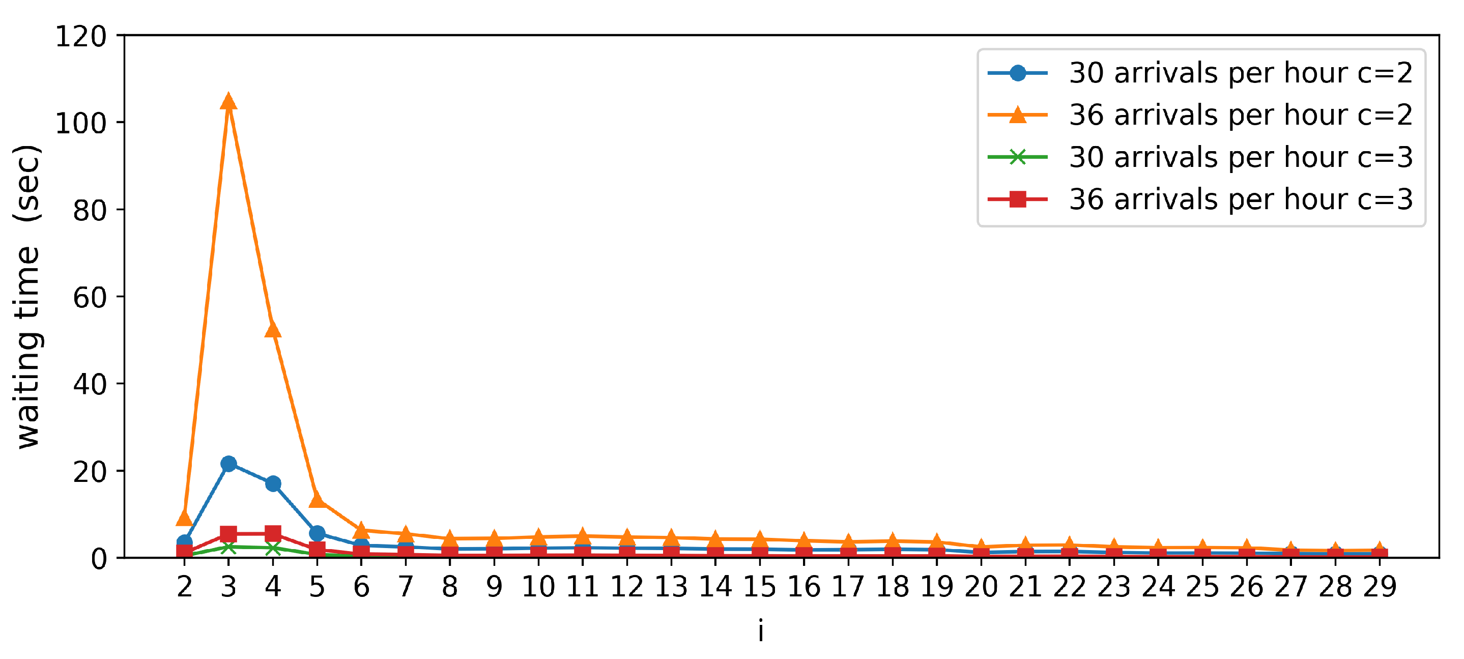
Table 5 and Table 6 show the estimated aircraft arrival delay when , as assumed for current operation and for Metering operation. Figure 14 compares the estimates for current operations and Metering operations under and . Comparing with the results of , the results show a remarkable reduction in arrival delay time, especially in the case of the airspace areas and . The respective arrival delays in areas and under current operations are and s, while under Metering operations the respective arrival delays are and s, as shown in Table 5 and Table 6. These results show that decreasing the minimum aircraft separation has a positive impact not only by increasing runway throughput, but also by decreasing arrival delay times in key airspace areas. The next section discusses how these benefits can be delivered.
6. Discussion
When arriving aircraft are flying far from the destination airport, the arrival traffic flow is controlled by airspace and airport capacity constraints. Close to the destination airport, flow control shifts to time-based arrival management in order to realize the required inter-arrival times between assigned aircraft arrival times. Applying a minimum inter-arrival aircraft time allows for an increased runway throughput. In this case, however, the most important questions are as follows: (i) How does decreasing inter-arrival aircraft time impact aircraft arrival delays? (ii) How can the arrival delay time be minimized while accommodating increasing air traffic demands? Below, we provide insight on these questions.
To address the first question, our queuing model for arrival traffic, with model parameters derived by analyzing actual flight data, yielded the following preliminary results: decreasing inter-arrival time is one of the most powerful solutions for reducing arrival delay times occurring in airspace bottleneck areas, and . Arrival delays can be remarkably reduced while allowing an increasing number of aircraft arrivals, as long as time-based separation can accommodate (i.e., three aircrafts present in a single airspace area at the same time), and as long as inter-aircraft separation can be reduced from that observed under current operations, i.e., a new wake vortex category is applied.
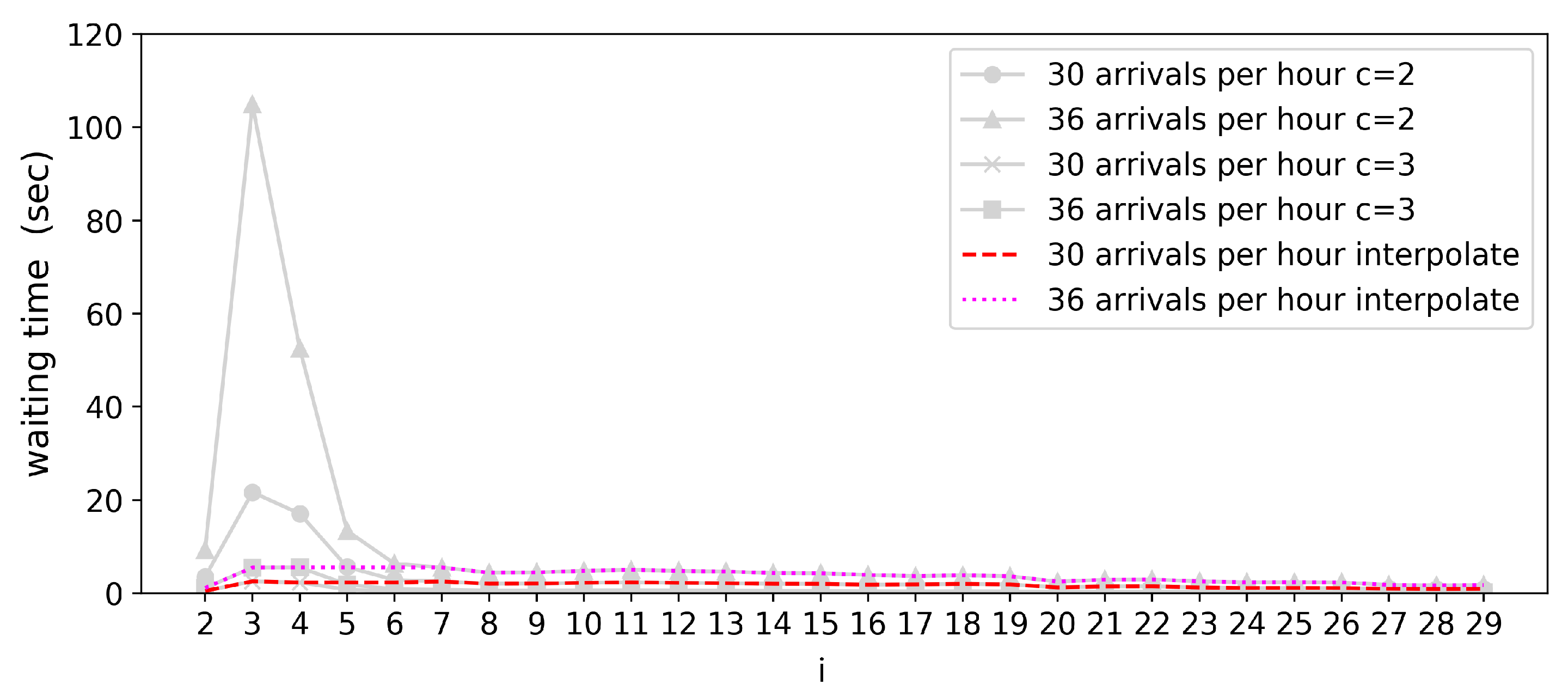
The second question can be addressed in a discussion of the transition point at which arrival management efficiently shifts from traffic flow control to time-based operation. Here, our arrival time delay estimates (see Figure 14) allow us to judge the transition point by smoothly interpolating the plots between and , as shown in Figure 15. This estimation shows that the most efficient transition will be realized around 70 NM distance from the airport.
Conventionally, improving automation levels in the future arrival management, i.e., applying aircraft self-separation and/or advanced AMAN, are discussed targeting increasing runway throughput, as shown in Section 4.2. However, their impacts on the overall arrival traffic flow have not been studied yet. This paper provides a quantitative approach which estimates bottlenecks and arrival delay time in the traffic flow as impacts of increasing runway throughput. Feasible solutions were clarified to achieve increasing arrival rate up to 120% (36 arrivals in an hour) while reducing arrival delay time for a case study airport. These results provide a meaningful practical value in the on-going process of developing global standards on the automation system design in air transport. The authors’ future work will estimate the maximum potential of arrival rates considering the automation levels and runway occupancy time at the airport under the latest air traffic data in 2019 corresponding the new configurations of airspace and air routes at the airport. The bottlenecks and feasible solutions will be clarified based on the proposed data-driven queuing approach.
Although the model is advantageous in clarifying these questions, mathematical restrictions prevent application of such models for operations in which the stability condition is not satisfied. As expressed in Equation (2), if the system workload is not less than 1, then the queue becomes unstable and the estimated delay time for incoming aircraft tends to become extraordinarily long. The second restriction of the model is the approximation accuracy of the estimated delay given by Equation (3): for a fixed c, the delay approximation provided in Equation (3) is asymptotically correct as approaches 1 [18], regardless of the values of and . Moreover, even for moderate values of , Equation (3) has been shown to be a good approximation, provided and [18]. As shown in Table 3, Table 4, Table 5 and Table 6, the queues considered for all 29 airspace areas satisfy the queue stability requirement. However, the value is not always close to 1, making the approximation of the delay less accurate, particularly in airspace far from the airport. To improve delay estimation accuracy, our future work will apply other queue-based modeling, and will compare estimation results with a macroscopic analysis of aircraft arrival by means of queuing models.
7. Conclusions
This paper proposes a queue-based modeling approach based on a data-driven analysis of radar tracks and flight plans in 2016 and 2017 at Tokyo International Airport. This analysis identifies bottleneck areas causing arrival delays. Mathematical analysis shows that reducing inter-aircraft arrival time is one helpful solution for reducing arrival time delays. This solution’s benefits would be delivered by efficiently shifting traffic flow control to arrival time management across a range of transition points. Fulfilling a key requirement of E-AMAN design, the most efficient range of transition points is estimated from the proposed data-driven queuing models, adopting values particular to each airport.
Currently, Tokyo International Airport’s reorganization of airspace and route structures is on-going, with promises of increasing passenger movement accompanying the Tokyo Olympic Games scheduled for 2020. We plan to verify our results in the context of this future increase in arrival traffic demand. We will apply our proposed approaches to analyses of arrival traffic at various airports whose individual properties differ from those of Tokyo International Airport. As such, different types of queuing models will be applied to further confirm the present paper’s results. Lastly, parameters in the queuing models will be optimized to indicate the ideal arrival traffic flow, not only targeting arrival delays but also mitigating economic and ecological impacts.
Author Contributions
The concept was proposed by E.I. The methodology was proposed by E.I. and M.M. Data curation and analysis was performed by E.I. The queuing model formal analysis was performed by M.M. and E.I. The article was written by E.I. and M.M. Funding was acquired by E.I.
Funding
This research was funded by Japan Civil Aviation Bureau (JCAB), Ministry of Land, Infrastructure, Transport and Tourism (MLIT) as the “Studies on the Extended Arrival Management” under CARATS initiatives. This research was also funded by the Ministry of Education, Culture, Sports, Science and Technology (MEXT) as the “Post-K Computer Exploratory Challenge (Exploratory Challenge 2: Construction of Models for Interaction Among Multiple Socioeconomic Phenomena, Model Development and its Applications for Enabling Robust and Optimized Social Transportation Systems) Project ID: hp180188”.
Acknowledgments
The authors are grateful to JCAB for providing air traffic data, and Mayumi Ohnuki for assisting data preparation and figure corrections. The authors would like to thank Enago (www.enago.jp) for the English language review.
Conflicts of Interest
The authors declare no conflict of interest.
References
- International Civil Aviation Organization. ICAO Long-Term Traffic Forecasts Passenger and Cargo, Total Passenger Traffic: History and Forecasts; International Civil Aviation Organization: Montreal, QC, Canada, 2016; 10p. [Google Scholar]
- Erzberger, H.; Itoh, E. Design Principles and Algorithms for Air Traffic Arrival Scheduling; NASA/TP-2014-218302; NASA Ames Research Center: Moffett Field, CA, USA, 2014.
- Federal Aviation Administration. NextGen Portfolio—Time Based Flow Management; Federal Aviation Administration: Washington, DC, USA, 2017.
- Thipphavong, J.; Jung, J.; Swenson, H.; Martin, L.; Lin, M.; Nguyen, J. Evaluation of the terminal sequencing and spacing system for performance-based navigation arrivals. In Proceedings of the 2013 IEEE/AIAA 32nd Digital Avionics Systems Conference (DASC), East Syracuse, NY, USA, 5–10 October 2013; p. 1A2-1-1A2-16. [Google Scholar]
- Van Tulder, P. Flight Deck Interval Management Flight Test Final Report; NASA/CR-2017-219626; NASA: Washington, DC, USA, 2017.
- European Commission. Cross Border SESAR Trials for Enhanced Arrival Management: Periodic Reporting for Period 1—PJ25 XSTREAM; European Commission: Brussels, Belgium, 2017.
- Sama, M.; D’Ariano, A.; Corman, F.; Pacciarelli, D. Metaheuristics for efficient aircraft scheduling and re-routing at busy terminal control areas. Trans. Res. Part C 2017, 80, 485–511. [Google Scholar] [CrossRef]
- International Civil Aviation Organization. Long Range Atfm Concept Trials. The Eighth Meeting of the ICAO Asia/Pacific Air Traffic Flow Management Steering Group (ATFMSG/8), May 2018. Available online: https://www.icao.int/APAC/Meetings/Pages/2018-ATFMSG8.aspx (accessed on 14 May 2018).
- Itoh, E.; Brown, M.; Senoguchi, A.; Wickramasinghe, N.; Fukushima, S. Future arrival management collaborating with trajectory-based operations. In Air Traffic Management and Systems II; Springer: Berlin, Germany, 2017; pp. 137–156. [Google Scholar]
- Modi, J.A. A nested queue model for the analysis of air traffic control sectors. Transp. Res. 1974, 8, 219–224. [Google Scholar] [CrossRef]
- Pyrgiotis, N.; Malone, K.M.; Odoni, A. Modelling delay propagation within an airport network. Transp. Res. Part C Emerg. Technol. 2013, 27, 60–75. [Google Scholar] [CrossRef]
- Menon, P.; Tandale, M.; Kim, J.; Sengupta, P. A Framework for Stochastic Air Traffic Flow Modeling and Analysis. In Proceedings of the AIAA Guidance, Navigation, and Control Conference, Toronto, ON, Canada, 2–5 August 2010; p. 7852. [Google Scholar]
- Simaiakis, I.; Balakrishnan, H. A queuing model of the airport departure process. Transp. Sci. 2015, 50, 94–109. [Google Scholar] [CrossRef]
- Idris, H.; Clarke, J.P.; Bhuva, R.; Kang, L. Queuing model for taxi-out time estimation. Air Traffic Control Q. 2002, 10, 1–22. [Google Scholar] [CrossRef]
- Bäuerle, N.; Engelhardt-Funke, O.; Kolonko, M. On the waiting time of arriving aircrafts and the capacity of airports with one or two runways. Eur. J. Oper. Res. 2007, 177, 1180–1196. [Google Scholar] [CrossRef] [Green Version]
- Long, D.; Lee, D.; Johnson, J.; Gaier, E.; Kostiuk, P. Modeling Air Traffic Management Technologies with a Queuing Network Model of the National Airspace System; NASA Langley Technical Report; NASA Langley Research Center: Hampton, VA, USA, 1999.
- Airports Council International. Passenger Traffic 2016 FINAL (Annual); Report 1 January 2018; Airports Council International: Montreal, QC, Canada, 2018. [Google Scholar]
- Whitt, W. The queueing network analyzer. Bell Syst. Tech. J. 1983, 62, 2779–2815. [Google Scholar] [CrossRef]
- Whitt, W. Approximations for the GI/G/m queue. Prod. Oper. Manag. 1993, 2, 114–161. [Google Scholar] [CrossRef]
- Kimura, T. A two-moment approximation for the mean waiting time in the GI/G/s queue. Manag. Sci. 1986, 32, 751–763. [Google Scholar] [CrossRef]
- Kingman, J. The single server queue in heavy traffic. In Mathematical Proceedings of the Cambridge Philosophical Society; Cambridge University Press: Cambridge, UK, 1961; Volume 57, pp. 902–904. [Google Scholar]
- Hillier, F.S. Introduction to Operations Research; Tata McGraw-Hill Education: New York, NY, USA, 2012. [Google Scholar]
- Adan, I.; Resing, J. Queuing Systems. 2015. Available online: https://www.win.tue.nl/~iadan/queueing.pdf (accessed on 15 September 2019).
- Little, J.D. A proof for the queuing formula. Oper. Res. 1961, 9, 383–387. [Google Scholar] [CrossRef]
- Arbuckle, D. Interval Management Application. In Proceedings of the ICAO Aircraft Surveillance Applications Workshop, Tokyo, Japan, 31 March 2017. [Google Scholar]
Figure 1.
Departure and arrival operations at Tokyo International Airport depending on the wind direction.
Figure 1.
Departure and arrival operations at Tokyo International Airport depending on the wind direction.

Figure 2.
Mean hourly numbers of flight departures and arrivals for each hour of the day, with standard deviations.
Figure 2.
Mean hourly numbers of flight departures and arrivals for each hour of the day, with standard deviations.

Figure 3.
Example record of flight tracks during an entire day in November 2016. The red tracks indicate traffic flow from southwest. The blue tracks indicate traffic flow from the north.
Figure 3.
Example record of flight tracks during an entire day in November 2016. The red tracks indicate traffic flow from southwest. The blue tracks indicate traffic flow from the north.

Figure 4.
Mean hourly numbers of total arrivals (blue), arrivals from southwest (red), and arrivals from the north (green), during each hour between 08:00 and 23:00, with standard deviations.
Figure 4.
Mean hourly numbers of total arrivals (blue), arrivals from southwest (red), and arrivals from the north (green), during each hour between 08:00 and 23:00, with standard deviations.

Figure 5.
Number of aircraft arrivals in an hour.

Figure 6.
Example of a queuing model for aircraft arrival traffic.

Figure 7.
Illustration of the service time and inter-arrival time-spacing.

Figure 8.
Distribution of service times with Gaussian fitting.

Figure 9.
Distribution of service times for each area i with Gaussian fitting, where area i is a circular ring centered on the airport and bounded by concentric circles of radii 10i and 10 NM.
Figure 9.
Distribution of service times for each area i with Gaussian fitting, where area i is a circular ring centered on the airport and bounded by concentric circles of radii 10i and 10 NM.

Figure 10.
Empirical distribution of the aircraft inter-arrival time and exponential fitting.

Figure 11.
Data-driven estimate of the number of servers, c, for the model.

Figure 12.
Future demand subject to increasing arrival rate.

Figure 13.
Comparison of the expected arrival delays for airspace capacity, .

Figure 14.
Comparison of the expected arrival delays for airspace capacities and .

Figure 15.
Interpolating the plots of waiting times between and .


Table 1.
Percentages of aircraft types among all aircraft arrivals.
| Types | B738 | B763 | B772 | A320 | B788 | B773 | B77W | B789 | A321 | B737 | A333 | E170 | A332 | B744 | B734 | Others |
|---|---|---|---|---|---|---|---|---|---|---|---|---|---|---|---|---|
| (%) | 34 | 18 | 14 | 10 | 6 | 3 | 3 | 2 | 2 | 2 | 2 | 1 | 0.6 | 0.5 | 0.4 | 0.8 |
Table 2.
Parameters of empirical distributions of the inter-arrival time and service time in seconds.
Table 2.
Parameters of empirical distributions of the inter-arrival time and service time in seconds.
| i | 1 | 2 | 3 | 4 | 5 | 6 | 7 | 8 | 9 | 10 |
|---|---|---|---|---|---|---|---|---|---|---|
| 111.5 | 112.4 | 111.8 | 108.9 | 108.3 | 107.3 | 106.7 | 106.2 | 106.3 | 106.8 | |
| 473.7 | 623.3 | 707.2 | 2607 | 3488 | 3720 | 4048 | 4267 | 4723 | 5489 | |
| 0.1951 | 0.2222 | 0.2377 | 0.4688 | 0.5451 | 0.5684 | 0.5960 | 0.6149 | 0.6467 | 0.6934 | |
| 219.7 | 153.7 | 186.0 | 163.2 | 121.9 | 99.24 | 93.18 | 86.11 | 83.84 | 82.07 | |
| 7016 | 508.5 | 3666 | 1640 | 331.9 | 177.1 | 181.6 | 154.5 | 179.5 | 183.2 | |
| 0.9853 | 0.6838 | 0.8313 | 0.7495 | 0.5626 | 0.4624 | 0.4364 | 0.4053 | 0.3944 | 0.3840 | |
| i | 11 | 12 | 13 | 14 | 15 | 16 | 17 | 18 | 19 | 20 |
| 107.1 | 107.1 | 107.1 | 107.0 | 107.7 | 107.9 | 110.6 | 111.1 | 111.2 | 111.1 | |
| 6252 | 6785 | 7259 | 7494 | 7691 | 7791 | 8080 | 8218 | 8264 | 8284 | |
| 0.7382 | 0.7689 | 0.7956 | 0.8089 | 0.8146 | 0.8182 | 0.8125 | 0.8160 | 0.8178 | 0.8193 | |
| 80.20 | 77.52 | 75.49 | 73.14 | 72.38 | 70.22 | 73.21 | 73.88 | 72.53 | 69.67 | |
| 153.0 | 106.3 | 75.71 | 70.09 | 65.20 | 63.38 | 74.33 | 84.20 | 84.75 | 76.95 | |
| 0.3744 | 0.3618 | 0.3524 | 0.3417 | 0.3362 | 0.3254 | 0.3309 | 0.3325 | 0.3262 | 0.3136 | |
| i | 21 | 22 | 23 | 24 | 25 | 26 | 27 | 28 | 29 | 30 |
| 118.5 | 119.0 | 120.0 | 122.1 | 122.4 | 125.1 | 125.6 | 132.5 | 135.8 | - | |
| 9345 | 9454 | 9542 | 9833 | 9822 | 10236 | 10313 | 11632 | 12168 | - | |
| 0.8157 | 0.8174 | 0.8160 | 0.8122 | 0.8099 | 0.8088 | 0.8088 | 0.8141 | 0.8126 | - | |
| 70.54 | 70.64 | 69.99 | 70.64 | 70.84 | 69.43 | 69.77 | 69.29 | 69.29 | - | |
| 61.90 | 65.22 | 61.94 | 65.85 | 74.39 | 59.45 | 58.36 | 56.76 | 55.99 | - | |
| 0.2976 | 0.2969 | 0.2923 | 0.2893 | 0.2894 | 0.2775 | 0.2778 | 0.2615 | 0.2552 | - |
Table 3.
Aircraft arrival delay and parameters of model for airspace capacity and arrival rate = 30 aircraft per hour.
Table 3.
Aircraft arrival delay and parameters of model for airspace capacity and arrival rate = 30 aircraft per hour.
| i | 1 | 2 | 3 | 4 | 5 | 6 | 7 | 8 | 9 | 10 |
|---|---|---|---|---|---|---|---|---|---|---|
| 101.4 | 3.461 | 21.66 | 17.05 | 5.606 | 2.828 | 2.497 | 2.017 | 2.060 | 2.219 | |
| 0.03289 | 0.04328 | 0.04911 | 0.1810 | 0.2422 | 0.2583 | 0.2811 | 0.2963 | 0.3280 | 0.3812 | |
| 0.1453 | 0.02152 | 0.1060 | 0.06155 | 0.02234 | 0.01798 | 0.02092 | 0.02084 | 0.02553 | 0.02720 | |
| 0.9155 | 0.6404 | 0.7748 | 0.6802 | 0.5079 | 0.4135 | 0.3883 | 0.3588 | 0.3493 | 0.3419 | |
| i | 11 | 12 | 13 | 14 | 15 | 16 | 17 | 18 | 19 | 20 |
| 2.309 | 2.207 | 2.144 | 1.997 | 1.979 | 1.821 | 1.876 | 1.970 | 1.869 | 1.230 | |
| 0.4341 | 0.4712 | 0.5041 | 0.5204 | 0.5341 | 0.5410 | 0.5243 | 0.5333 | 0.5363 | 0.4660 | |
| 0.02378 | 0.01770 | 0.01329 | 0.01310 | 0.01245 | 0.01285 | 0.01387 | 0.01543 | 0.01611 | 0.01585 | |
| 0.3342 | 0.3230 | 0.3145 | 0.3047 | 0.3016 | 0.2926 | 0.2949 | 0.2976 | 0.2921 | 0.2613 | |
| i | 21 | 22 | 23 | 24 | 25 | 26 | 27 | 28 | 29 | 30 |
| 1.428 | 1.452 | 1.219 | 1.102 | 1.114 | 1.084 | 0.9381 | 0.8687 | 0.9073 | - | |
| 0.5256 | 0.5318 | 0.4977 | 0.4742 | 0.4737 | 0.4936 | 0.4584 | 0.4748 | 0.4967 | - | |
| 0.01244 | 0.01307 | 0.01264 | 0.01320 | 0.01483 | 0.01233 | 0.01199 | 0.01182 | 0.01166 | - | |
| 0.2645 | 0.2649 | 0.2527 | 0.2453 | 0.2460 | 0.2411 | 0.2326 | 0.2214 | 0.2213 | - |
Table 4.
Aircraft arrival delay and parameters of the model, , arrival rate = 36 aircraft per hour.
| i | 1 | 2 | 3 | 4 | 5 | 6 | 7 | 8 | 9 | 10 |
|---|---|---|---|---|---|---|---|---|---|---|
| − | 9.292 | 104.9 | 52.49 | 13.37 | 6.321 | 5.499 | 4.385 | 4.450 | 4.787 | |
| 0.04737 | 0.06233 | 0.07072 | 0.2607 | 0.3488 | 0.3720 | 0.4048 | 0.4267 | 0.4723 | 0.5489 | |
| 0.1453 | 0.02152 | 0.1060 | 0.06155 | 0.02234 | 0.01798 | 0.02092 | 0.02084 | 0.02553 | 0.02720 | |
| 1.099 | 0.7684 | 0.9298 | 0.8162 | 0.6095 | 0.4962 | 0.4659 | 0.4306 | 0.4192 | 0.4103 | |
| i | 11 | 12 | 13 | 14 | 15 | 16 | 17 | 18 | 19 | 20 |
| 4.987 | 4.770 | 4.635 | 4.305 | 4.263 | 3.910 | 3.650 | 3.832 | 3.630 | 2.476 | |
| 0.625 | 0.6785 | 0.7259 | 0.7494 | 0.7691 | 0.7791 | 0.7207 | 0.7330 | 0.7371 | 0.6545 | |
| 0.02378 | 0.01770 | 0.01329 | 0.01310 | 0.01245 | 0.01285 | 0.01387 | 0.01543 | 0.01611 | 0.01585 | |
| 0.4010 | 0.3876 | 0.3774 | 0.3657 | 0.3619 | 0.3511 | 0.3457 | 0.3489 | 0.3425 | 0.3096 | |
| i | 21 | 22 | 23 | 24 | 25 | 26 | 27 | 28 | 29 | 30 |
| 2.887 | 2.935 | 2.518 | 2.332 | 2.356 | 2.292 | 1.763 | 1.671 | 1.746 | - | |
| 0.7384 | 0.7470 | 0.7076 | 0.6829 | 0.6821 | 0.7108 | 0.6239 | 0.6544 | 0.6845 | - | |
| 0.01244 | 0.01307 | 0.01264 | 0.01320 | 0.01483 | 0.01233 | 0.01199 | 0.01182 | 0.01166 | - | |
| 0.3135 | 0.3139 | 0.3014 | 0.2943 | 0.2952 | 0.2893 | 0.2713 | 0.2598 | 0.2598 | - |
Table 5.
Aircraft arrival delay and parameters of the model for airspace capacity and arrival rate = 30 aircraft per hour.
Table 5.
Aircraft arrival delay and parameters of the model for airspace capacity and arrival rate = 30 aircraft per hour.
| i | 1 | 2 | 3 | 4 | 5 | 6 | 7 | 8 | 9 | 10 |
|---|---|---|---|---|---|---|---|---|---|---|
| 6.165 | 0.4768 | 2.535 | 2.287 | 0.7678 | 0.3572 | 0.3052 | 0.2356 | 0.2366 | 0.2515 | |
| 0.03289 | 0.04328 | 0.04911 | 0.1810 | 0.2422 | 0.2583 | 0.2811 | 0.2963 | 0.3280 | 0.3812 | |
| 0.1453 | 0.02153 | 0.1060 | 0.06155 | 0.02234 | 0.01798 | 0.02092 | 0.02084 | 0.02553 | 0.02720 | |
| 0.6103 | 0.4269 | 0.5166 | 0.4535 | 0.3386 | 0.2757 | 0.2588 | 0.2392 | 0.2329 | 0.2280 | |
| i | 11 | 12 | 13 | 14 | 15 | 16 | 17 | 18 | 19 | 20 |
| 0.2578 | 0.2411 | 0.2301 | 0.2097 | 0.2063 | 0.1859 | 0.1926 | 0.2034 | 0.1906 | 0.1156 | |
| 0.4341 | 0.4712 | 0.5041 | 0.5204 | 0.5341 | 0.5410 | 0.5243 | 0.5333 | 0.5363 | 0.4660 | |
| 0.02378 | 0.01770 | 0.01329 | 0.01310 | 0.01245 | 0.01285 | 0.01387 | 0.01543 | 0.01611 | 0.01585 | |
| 0.2228 | 0.2153 | 0.2097 | 0.2031 | 0.2011 | 0.1950 | 0.1966 | 0.1984 | 0.1948 | 0.1742 | |
| i | 21 | 22 | 23 | 24 | 25 | 26 | 27 | 28 | 29 | 30 |
| 0.1355 | 0.1379 | 0.1117 | 0.09874 | 0.1000 | 0.09579 | 0.08064 | 0.07181 | 0.07499 | - | |
| 0.5256 | 0.5317 | 0.4977 | 0.4742 | 0.4736 | 0.4936 | 0.4584 | 0.4748 | 0.4967 | - | |
| 0.01244 | 0.01307 | 0.01264 | 0.01320 | 0.01483 | 0.01233 | 0.01199 | 0.01182 | 0.01166 | - | |
| 0.1764 | 0.1766 | 0.1685 | 0.1635 | 0.1640 | 0.1607 | 0.1550 | 0.1476 | 0.1476 | - |
Table 6.
Aircraft arrival delay and parameters of the model, , arrival rate = 36 aircraft per hour.
| i | 1 | 2 | 3 | 4 | 5 | 6 | 7 | 8 | 9 | 10 |
|---|---|---|---|---|---|---|---|---|---|---|
| 14.26 | 1.102 | 5.484 | 5.506 | 1.861 | 0.8601 | 0.7324 | 0.5648 | 0.5658 | 0.6022 | |
| 0.04736 | 0.06233 | 0.07072 | 0.2607 | 0.3488 | 0.3720 | 0.4048 | 0.4267 | 0.4723 | 0.5489 | |
| 0.1453 | 0.02153 | 0.1060 | 0.06155 | 0.02234 | 0.01798 | 0.02092 | 0.02084 | 0.02553 | 0.02720 | |
| 0.7324 | 0.5123 | 0.6199 | 0.5441 | 0.4063 | 0.3308 | 0.3106 | 0.2870 | 0.2795 | 0.2736 | |
| i | 11 | 12 | 13 | 14 | 15 | 16 | 17 | 18 | 19 | 20 |
| 0.6201 | 0.5824 | 0.5575 | 0.5083 | 0.5003 | 0.4505 | 0.4165 | 0.4398 | 0.4118 | 0.2629 | |
| 0.6252 | 0.6785 | 0.7259 | 0.7494 | 0.7691 | 0.7791 | 0.7207 | 0.7330 | 0.7371 | 0.6545 | |
| 0.02378 | 0.01770 | 0.01329 | 0.01310 | 0.01245 | 0.01285 | 0.01387 | 0.01543 | 0.01611 | 0.01585 | |
| 0.2673 | 0.2584 | 0.2516 | 0.2438 | 0.2413 | 0.2341 | 0.2305 | 0.2326 | 0.2283 | 0.2064 | |
| i | 21 | 22 | 23 | 24 | 25 | 26 | 27 | 28 | 29 | 30 |
| 0.3091 | 0.3145 | 0.2623 | 0.2391 | 0.2419 | 0.2321 | 0.1704 | 0.1564 | 0.1635 | - | |
| 0.7384 | 0.7470 | 0.7076 | 0.6829 | 0.6821 | 0.7108 | 0.6239 | 0.6543 | 0.6845 | - | |
| 0.01244 | 0.01307 | 0.01264 | 0.01320 | 0.01483 | 0.01233 | 0.01199 | 0.01182 | 0.01166 | - | |
| 0.2090 | 0.2093 | 0.2009 | 0.1962 | 0.1968 | 0.1928 | 0.1809 | 0.1732 | 0.1732 | - |
© 2019 by the authors. Licensee MDPI, Basel, Switzerland. This article is an open access article distributed under the terms and conditions of the Creative Commons Attribution (CC BY) license (http://creativecommons.org/licenses/by/4.0/).
Share and Cite
MDPI and ACS Style
Itoh, E.; Mitici, M. Queue-Based Modeling of the Aircraft Arrival Process at a Single Airport. Aerospace 2019, 6, 103. https://doi.org/10.3390/aerospace6100103
AMA Style
Itoh E, Mitici M. Queue-Based Modeling of the Aircraft Arrival Process at a Single Airport. Aerospace. 2019; 6(10):103. https://doi.org/10.3390/aerospace6100103
Chicago/Turabian StyleItoh, Eri, and Mihaela Mitici. 2019. "Queue-Based Modeling of the Aircraft Arrival Process at a Single Airport" Aerospace 6, no. 10: 103. https://doi.org/10.3390/aerospace6100103
Note that from the first issue of 2016, this journal uses article numbers instead of page numbers. See further details here.