1. Introduction
Designing and building systems to operate in a space environment is a complex and demanding engineering challenge. Reproducing all conditions encountered in space before the launch of the spacecrafts into orbit is not feasible. Correcting faults on any orbiting spacecraft is extremely costly and usually not an option. Therefore, spacecraft designers must go to great lengths to ensure the safe operation of their system in an environment they were never able to test in. For flight software testing, hardware-in-the-loop (HIL) and software-in-the-loop (SIL) simulations are widely used verification methods [
1]. In addition to the software verification, HIL simulations also cover some of the hardware of the satellite, which might include the processor with its peripheral electronics, the sensors, and actuators. Most literature about simulations for CubeSat and small satellite verification focuses on the attitude determination and control system (ADCS). One approach towards ADCS simulation utilizes facilities resembling the physical characteristics of the space environment, like Helmholtz cages, sun simulators, and air bearings, allowing the ADCS to utilize its real sensors and actuators [
2,
3,
4]. Another approach is replacing the real sensors and actuators with simulation models and using the corresponding subsystems in hardware [
5] or simulating all of the hardware of the satellite to verify the flight software and train operators [
6,
7].
Both HIL and SIL contributed to the development and verification of MOVE-II’s ADCS. For MOVE-II’s Electrical Power System (EPS) and the safe mode switching implemented on the Command & Data Handling (CDH), we exclusively used HIL testing for verification.
In comparison to other CubeSat simulation approaches, the MOVE-II HIL environment implements both digital sensor signals and electric voltages to provide a useful interface to ADCS and EPS simultaneously. Including the electrical domain enables the developers to discover errors caused by the interaction between ADCS and EPS. Another novelty is the application of HIL simulations for augmenting the operator training with realistic failure scenarios and accurate reaction to the operator’s commands.
MOVE-II, the Munich Orbital Verification Experiment II, is a 1.2 kg, 1U CubeSat developed from April 2015 onwards at the Technical University of Munich and launched into space on 3 December 2018 [
8]. Like its predecessor First-MOVE, MOVE-II was designed, built, and is currently operated mainly by students at the Technical University of Munich. Lessons learned from MOVE-II’s first months of operations were implemented on a twin-satellite, called MOVE-IIb, which was launched on July 5th, 2019. From the beginning of the development of the MOVE-II satellites, lessons learned from First-MOVE and other CubeSat teams [
9,
10] were implemented in the program. We followed a development approach similar to the Bread–Brass–Silver–Gold approach of the Air Force Research Laboratory’s University Nanosatellite Program [
11,
12].
MOVE-II features an active magnetorquer-based ADCS, which is based on six printed circuit boards (depicted in
Figure 1). All boards feature integrated magnetorquers, coil driving electronics, a gyroscope, a magnetometer, and a microcontroller. The Sidepanels, as well as the Toppanel, include individual sun sensors. Each of the satellite’s body axes feature a magnetorquer, resulting in redundancy of the actuation system.
Figure 2 illustrates the corresponding body-fixed coordinate system.
The ADCS features two different control modes, both of which are mission-critical: First, to slow down the initial angular velocity of the satellite after separation from the CubeSat deployer, a detumbling maneuver has to be executed, using a B-dot control algorithm [
13]. The second control mode is sun-pointing, for which a linear model-based controller is used to direct the payload on the Toppanel and the solar cells of the satellite towards the sun to ensure enough power generation and successful payload measurements. A spin around the z-axis stabilizes the pointing vector [
14]. The state vector for the controller can be either directly attained by sensor measurements or by estimation. For the latter option, an Extended Kalman Filter (EKF) is implemented. Thus, sensor data is fused together to provide an estimation of the satellite’s attitude. More information on the ADCS of MOVE-II as well as its control strategies used can be found in [
15].
The EPS of MOVE-II features four deployable solar panels that are populated with two cells each and provide a peak power of 10 W. Once deployed, they all point in the same direction (negative z-axis, see
Figure 2) and are the main source of power income for the satellite. Additionally, the Sidepanels are populated with two smaller cells each, providing backup power if the satellite is tumbling. The solar cells are grouped in three arrays and charge the battery of the satellite over maximum power point trackers.
To derive a suitable system architecture for our simulation, we do not divide the satellite into several subsystems, but into the domains: Processing, Interfaces, and Physics.
Figure 3 shows these domains plus the space environment that the satellite is interacting with. All of the satellite’s software and most of the satellite’s hardware, grouped in the block Processing, is not significantly affected by the space environment, at least not during the time frame of a simulation, i.e., less than 24 h. All hardware components with a significant dependence on the environment’s physical stimuli are grouped in the block Interfaces, separate from the rest of the satellite’s hardware. The interfaces include sensors, solar cells, etc., but also a battery that significantly increases its internal resistance at low temperatures, which qualifies as an interface. The block Physics comprises the satellite’s physical properties like the inertia tensor or its thermal capacitance and is an intermediary between the space environment and the satellite’s interfaces. The block “Space Environment” contains all external stimuli influencing the satellite.
2. The Simulation Environment of MOVE-II
HIL simulations enjoy widespread use in the small satellite community, especially for ADCS verification. Many teams opt for a physical approach for the simulation of the space environment, utilizing air bearing platforms with attitude sensors to enable quasi-frictionless rotation, Helmholtz cages for the simulation of the magnetic field of the Earth, and sunlight simulators [
2,
3]. This setup allows the teams to perform HIL tests by mounting ADCS sensors and actuators for testing generic attitude control and estimation algorithms [
16], or using flight components by simply mounting the desired sensor or actuator onto the platform [
4].
Another strategy is to use a numerical simulation of the space environment, replacing the real sensors with models by mimicking their signals and sending them to the actual control computer. To simulate the effect of the actuation and close the loop, the commands for the actuators generated by the control computer are read or, in the case of magnetorquers, it is also possible to measure the actual response of the actuators, in order to account for transient behavior, nonlinearity, and uncertainty of the magnetorquers [
17]. This means that the space environment is not replicated in a physical way and interacting with the satellite’s hardware. Instead, the space environment is simulated and the sensor’s values are computed and sent to the control computer, and the effect of the actuation is also simulated.
More processing hardware than just that of the ADCS can be included in the simulations [
5], for example, power units connected to the EPS board, emulating the voltage and current supplied by each solar panel, information which can be obtained based on the simulated thermal flow in the satellite, and the temperatures on the solar panels, together with information of sun position and the satellite attitude [
18].
Another approach is simulating most, or even all, of the hardware of the satellite [
7], executing the software as if it were operating in space, with simulated data inputs, to verify the flight software and/or train operators [
6].
With their varying levels of hardware coverage and different ways to inject fault conditions, all these approaches result in different regions of test coverage and complement each other. For the MOVE-II simulation environment, we combined real processing hardware with simulated sensors, mimicking their signals, and simulated actuators commanded by the response of the processing hardware.
Adhering to the abstract model depicted in
Figure 3, we placed the simulation boundary between the interfaces and processing as shown in
Figure 4. This means that the simulation discussed in
Section 2.2 covers the domains Space Environment, Physics, and Interfaces. The simulation environment only includes the processing hardware as device-under-test. To achieve full coverage, we must combine the simulation-based verification of this HIL environment with separate additional tests of the sensors and actuators in, e.g., a Helmholtz cage. We selected this test approach for MOVE-II, because we are mainly interested in verifying the software and controllers in an integrated configuration.
2.1. Overview
MOVE-II’s HIL environment includes a simulation containing the space environment, physics, interface models of the ADCS and EPS, and temperature sensors for CDH. It also computes the distance and orientation to the ground station for the channel simulator.
Table 1 lists all interface emulators forwarding the simulated interface data to the processing hardware of the satellite. The processing hardware consists of the stack of subsystem boards of MOVE-II’s engineering model. The Sidepanels, the Toppanel, and the antennas were disconnected. All components except the PC running the simulation and the ground station containing the channel simulator are shown in
Figure 5.
The following sections will give a detailed description of the MOVE-II HIL environment used for verifying the satellite’s software and power budget.
Section 2.2 covers the simulation model,
Section 2.3 lists the interface emulators, and
Section 2.4 shows how we can use the same environment for HIL, SIL, and simple simulations.
Section 2.5 shows the types of data exchanged in the HIL environment, and
Section 2.6 gives the most significant characteristics of the test environment.
2.2. Simulation
The complete simulation is implemented in Matlab/Simulink. Space environmental aspects, the satellite’s physical properties, sensors, and actuators are modeled as blocks in a Simulink model.
Figure 6 gives an overview of the top-level structure of the Simulink environment.
The block Space Environment incorporates a magnetic field model, a sun position model including Earth’s eclipse, and an orbit propagator. It outputs a magnetic field vector
, a sun vector
, the position vector
, velocity vector
, and the angle to the ground station
, respectively. All vectors are in the body frame of the satellite depicted in
Figure 2. A satellite dynamics model and a simple thermal model describe the satellite’s physical state. They calculate the angular velocity
, the attitude quaternion
, and the temperature
of the satellite. The environmental information and the satellite’s physical state are forwarded to the Sensor Models block, which provides measurements of the sun vector
, magnetic field vector
, angular velocity vector
, and of the temperature
.
Section 2.2.1 will cover the sensor models of this block. The temperature measurement is forwarded to the Universal Interface Node (UIN), whereas the ADCS sensor measurements are forwarded to the Panel Emulator. The Solar Array Simulator sends the power of the maximum power point (MPP), denoted as the available power
, and the power actually drawn by the battery charge regulator, the accepted power
, for every of the three channels to the simulation PC. The quotient of these two values yields the instantaneous maximum power point tracking efficiency of the EPS.
The Power Estimator uses , , , and the actuator currents (not included in the diagram for simplicity) to compute the overall power dissipation and the solar intensity . The Channel Simulator requires the orbital position vector and the velocity vector of the satellite as well as its angle with respect to the ground station.
The ADCS sensor data forwarded to the Panel Emulator is processed on the ADCS Mainpanel. The desired control currents
from the control algorithms are forwarded back to the simulation and used within the Actuator Models to compute the control torque vector
. This torque plus the disturbance torques from the Disturbances model
are input to the Rotational Dynamics model. The modeled disturbances include residual magnetic dipole moment, drag caused by the residual atmosphere, the gravity gradient disturbance, and a magnetic dipole moment disturbance induced by the illumination of the solar panels [
19].
Besides the HIL interface, the simulation environment provides two more possibilities to close the control loop for the ADCS: The first approach is using a simple Simulink model of the contol law being used. This is denoted by in
Figure 6. The second approach incorporates the firmware implementation of the control strategy in the simulation environment. Therefore, the C++ code of the algorithms are embedded in Level-2 S-functions which are included as a block into the Simulink model (denoted by Controller Software in
Figure 6). This block exchanges data with the remaining Simulink blocks. This method is referred to as Software-in-the-Loop. The corresponding control current outputs for these approaches are denoted as
and
, respectively. These different approaches can be also applied on the estimation part of the ADCS. More information on these different approaches is given in
Section 2.4.
2.2.1. Sensor Models
All the sensor models follow the same principle. At first, a reference value is calculated by the simulation. In our simulation environment, the reference values are the magnetic field vector
, the sun vector
, the angular velocity
, and the temperature
. Then, to model a magnetometer, a sun sensor, a gyroscope, and a temperature sensor, respectively, some realistic aspects are considered. For all ADCS related sensors models, the reference values are sampled and rotated into the sensor frame. In the specific context of vector measurements
and
, the true satellite attitude
is required to rotate the reference vectors into the satellite’s body fixed frame before being transformed into their sensor frames. To model the measurements, various errors are introduced to represent the various inaccuracies in the sensor. This may include white noise, bias, scaling, and misalignment errors. The output of the sensor model is then discretized to introduce quantization errors to emulate a digital signal.
Table 2 gives an overview of the modeled effects for the magnetometer, gyroscope, the sun sensor, and the temperature sensor.
Deterministic parameters such as scaling and bias as well as noise characteristics are estimated using recordings of real sensor measurements. To validate the sensor models, the real sensor measurements were compared to readings produced by the simulation. The recordings where both compared in the time and frequency domains.
2.2.2. Controller Models
The simulation environment enables students to develop and test a variety of attitude determination and control algorithms and to evaluate them as a part of the firmware of MOVE-II. It is difficult to predict the behavior of control laws solely with analytical methods. Linearized controllers in particular often show unwanted or unexpected behavior far away from their operation point.
Table 3 lists all attitude determination and control algorithms that have been evaluated in our simulation environment and the section that explains the algorithm’s verification in more detail.
Section 2.4 gives an overview on the simulation approaches mentioned in the third column. The simulation approaches are Ideal Simulation (IS), Realistic Simulation (RS), SIL, and HIL. All algorithms, which are included in the flight software of either MOVE-II or MOVE-IIb, are verified in the HIL configuration of the environment.
2.3. Hardware Interfaces
Replacing the interfaces of the satellite with simulation models requires physical hardware interfaces that translate the data of the simulation to the electrical buses of the processing hardware. The following interface emulators allow the simulation to talk to the ADCS, the maximum power point (MPP) trackers of the EPS, and the CDH. Additionally, the channel simulator controls the properties of the transceiver’s (COM) communication channel to the ground station.
2.3.1. Panel Emulator
The Panel Emulator connects the simulation and the ADCS of the satellite [
20]. As explained in
Section 1, the ADCS of MOVE-II is comprised of the Mainpanel, five Sidepanels, and the Toppanel. The Mainpanel runs the attitude determination and control algorithms. The Sidepanels and the Toppanel house the sensors and actuators as well as a microcontroller for controlling them. The Mainpanel reads the sensor values and writes the actuator commands via direct memory access (DMA). The Panel Emulator replaces the Sidepanels and the Toppanel by utilizing five microcontrollers that mimic the individual panels and relay the sensor and actuator values via SPI to a Beaglebone running Debian Linux. The Beaglebone connects over Ethernet to the simulation PC. A python script on the simulation PC talks over UDP to the simulation and over WebSockets to the Panel Emulator Beaglebone. On the Beaglebone, a C++ program acts as relay between the WebSockets connection and the SPI bus to the microcontrollers.
For power budget verification, the wiring between the Panel Emulator and the Mainpanel also provides a read-only connector for the real Sidepanels and the Toppanel. Thus, the real panels will receive and execute the commands from the Mainpanel; however, the pin for sending sensor readings to the Mainpanel is not connected. Therefore, the real panels will consume a realistic amount of power but will not interfere with the communication between Panel Emulator and Mainpanel.
2.3.2. Solar Array Simulator
The Solar Array Simulator interfaces between the satellite’s EPS and the simulation [
21]. In general, Solar Array Simulators are special power supplies that replicate the electrical behavior of a solar array, which can be described by a voltage–current characteristic curve (VI curve). The VI curve of a solar array defines its output current as a function of its output voltage and is dependent both on the illumination level and on the temperature of the photovoltaic cells in the array. The Solar Array Simulator in the HIL setup communicates to the simulation PC via Ethernet. In every simulation cycle, the Solar Array Simulator receives the current illumination level and temperature of each solar cell and computes the VI curves of the three solar arrays of MOVE-II based on that information using a method described in [
22]. The Solar Array Simulator then drives its three output channels to behave according to the determined curves. The output channels of the Solar Array Simulator are connected to the three battery charging regulators of the EPS. The exact voltage and current supplied by a certain channel, i.e., the operating point on the simulated VI curve is determined by the load represented by the respective battery charge regulator. The EPS tries to set this operating point to the maximum power point of the VI curve where the most power possible is extracted from the solar array or Solar Array Simulator.
2.3.3. Connection to CDH
The CDH of MOVE-II runs the main state machine controlling the mode of ADCS and EPS and reads out the temperature sensors of the satellite. The simulation can send commands to CDH during setup to set the time and the mode of all relevant subsystems. The simulation also allows commanding CDH during the run, e.g., switching the gain of ADCS in eclipse. Sending commands to CDH is possible over three different methods:
Serial link: The satellite allows commanding CDH directly in integrated configuration over the External Debug Interface (EDI). EDI includes a UART link to the CDH that the simulation PC can use over a UART-USB converter. This connection is easy to setup and does not significantly disturb the power budget of the satellite.
Mission Control: The simulation registers as a user at the operations interface of the satellite. The operations interface sends the command over the experimental ground station in the integration room to the transceiver of the satellite and the CDH executes it. This connection is very realistic regarding the hardware involved, but significantly impedes the power budget due to the higher power consumption of the satellite’s transceiver when a ground station is in sight.
Low-cost CDH: MOVE-II’s CDH was a commercial component that was only bought for the Engineering-Model and the Flight-Models of MOVE-II and MOVE-IIb. To overcome the shortage of hardware, the team built a Beaglebone-based low-cost CDH with a PC/104 connector that runs the MOVE-II Linux operating system plus all software controlling the subsystems [
8]. This cheap and simple solution found its way into many prototypes of the satellite including several HIL setups. The simulation can login to the low-cost CDH over SSH and issue commands.
2.3.4. Universal Interface Node
The multitude of processing nodes involved in the links of the simulation to ADCS and EPS introduces a high latency of more than 100 ms. Also, WebSocket uses TCP, and therefore has more latency than UDP communication. As an effort to simplify the connection between simulation and hardware, the universal interface node uses only one device translating from UDP packets sent by the simulation to the bus of the device under test. Instead of defining a fixed packet format, the simulation serializes and packetizes the sensor values using Google Protobuf. The UIN is in development and only allows for communication over the buses Onewire and SPI at the time of writing. Multiple UINs emulate a subset of MOVE-II’s temperature sensors, which are read out by the CDH.
2.3.5. Channel Simulator
The RF link between the ground station and the satellite heavily impedes operations, especially when the satellite is tumbling or using a directional antenna that needs to track the ground station. The Channel Simulator is a GNU radio block that adds Doppler shift and dampening to the digital signal depending on the satellite’s range, orientation, and velocity with regard to the ground station. The antennas of the satellite and the experimental ground station in the integration are replaced with an RF cable and an attenuator. The channel simulator block can run on the ground station PC or on a PC with a separate SDR (software-defined radio). The channel simulator is a work in progress and will be included in a future iteration of the HIL setup.
2.4. Simulation Approaches
The simulation environment is capable of executing different simulation approaches by deactivating blocks and rerouting signals in the Simulink model shown in
Figure 6:
Ideal Simulation (IS): The Simulink model only considers the minimum set of blocks to build a control loop. Therefore, the Sensor Models, Actuator Models, and Disturbances blocks are deactivated. The selected controller block is Simulated Controller.
Realistic Simulation (RS): The Simulink models considers a high-fidelity space environment, sensor and actuator models. Again, the selected controller block is Simulated Controller.
Software-in-the-Loop (SIL): The control algorithm implemented in C++ code processes the sensor readings. This algorithm is implemented in the block Controller Software. The C++ code of the algorithm is part of the ADCS firmware. Therefore, parts of the flight firmware can be tested within the simulation environment.
Hardware-in-the-Loop (HIL): This approach incorporates the satellite hardware into the setup as depicted in
Figure 4. Algorithms are no longer directly implemented in the Simulation environment, but on the satellite hardware. Simulations in HIL run at real-time, and are therefore substantially slower than in any of the less extensive approaches above.
By default, the simulation approaches RS, SIL, and HIL include all models, whereas the IS approach only includes a minimum set as mentioned before. If desired, the user may choose whether to disable any of the models or to change specific simulation parameters for these models.
The simulation allows a user to easily switch between the different approaches depending on the purpose of the test run. These methods provide a wide range of possibilities to verify and test algorithms or other aspects under different perspectives. The IS method provides a very simple simulation framework for a first proof-of-concept of algorithms such as control laws. Using the RS method, we can utilize the high-fidelity implementation of models. This allows simulating algorithms implemented in Matlab/Simulink under more realistic conditions. As opposed to the IS method, the simulation speed of the RS method can be significantly slower. For the SIL method, we embed the code algorithms in a Simulink block by using Level-2 S-functions. As depicted in
Figure 4, these blocks containing the code can be connected to the remaining blocks of the Simulink model. Thus, the software implementation of an algorithm can be easily verified and tested with simulated inputs. Finally, the HIL approach utilizes the processing hardware on which the algorithms are implemented. This allows us to account for hardware-related issues that are not considered in the other methods. However, due to the implementation of the HIL setup, delays and roundtrip times can affect the simulation output, as described later in
Section 2.6.
Table 4 gives an overview of the objectives and constraints for each method.
The development and verification process of an algorithm typically starts with the IS approach and ends with the HIL approach. The implementation of an algorithm in Matlab/Simulink is rather easy, allowing the developer to evaluate new concepts and ideas in short time. In a next step, the performance of these algorithms can be investigated in more detail using the RS approach. The simulations can be executed a lot faster than real-time allowing evaluation of the long-term stability. If the algorithm shows promising results, one may decide to implement it in C++ code and integrate it into the simulation via the SIL approach. The software modules are verified for correct implementation. The last step is a HIL verification where the algorithms are finally implemented in the firmware of the ADCS Mainpanel.
Before starting a simulation, one can choose to do a single run or to enter a special simulation mode. These special modes are useful for performing several simulations automatically at once. They are especially interesting when evaluating control algorithms, but they also can be used for different analysis like determining the power budget of the satellite. The modes are introduced in the following.
A list with test cases. Each test case specifies a set of simulation parameters. The simulation will run through all test cases until the list is finished in one go.
A Monte Carlo simulation with randomized initial attitude and angular velocity. This simulation helps in analyzing the convergence behavior of a control algorithm with respect to varying initial conditions. Both the average convergence time as well as the probability of convergence are measured.
A sensitivity analysis, where multiple simulation parameters are varied over a preset value range. This simulation mode reveals if the controller is robust to environmental changes and deviations from the target orbit.
We use Matlab/Simulink for editing the simulation and adjusting its parameters. The user selects the correct settings and simulation parameters in a Matlab script. This script calls different functions which set the interface emulators to the correct mode, initialize the Simulink model and issue commands to the satellite’s CDH. Afterwards, depending on the selected settings, the specified series of simulations is executed automatically.
2.5. Data Flows
Figure 7 shows the components mentioned in the previous section including the type of connection and the transferred information. Most connections carry digital signals. Only the interface to EPS includes analog voltages mimicking an array of solar cells. The Panel Emulator translates from WebSockets to the ADCS’s SPI bus, and the Solar Array Simulator translates from WebSockets to the VI curve that the EPS’s MPP trackers expect. Both the Panel Emulator and the Solar Array Simulator use a dedicated WebSockets server that connects to the simulation via UDP messages. The Universal Interface Nodes translates directly from UDP to the CDH’s Onewire bus. Also, the Channel Simulator uses UDP messages for connecting to the simulation.
2.6. Characteristics of the HIL Environment
As jitter is introduced by the timing of the simulation steps running on an asynchronous operating system and the network roundtrip times vary, two runs with the same parameters will never yield the exact same results. Moreover, only a Simulation Pace block in the Simulink model slows down the execution time to real-time. We can show that the repeat accuracy is better than
when considering the pointing error for a run of two orbits [
20]. The reference here is a test case demonstrating Spinning Sunpointing with all disturbances on realistic level. The longer the simulation, the bigger the difference between two runs with the same parameters; therefore, the HIL environment is not suitable for conducting sensitivity analyses of highly accurate attitude control systems. To overcome this limitation in the future, the simulation needs a dedicated real-time target and the interface emulators need to use low-latency protocols, similar to the Universal Interface Node. The round-trip-time between simulation and Panel Emulator is 300
with the maximum sample time in the simulation set to 50
. If one assumes that a change in attitude below 10° can be considered insignificant, the maximum angular velocity of the satellite should never exceed 33 °/s. Simulations at higher velocities will always suffer significantly from delays and jitter introduced by the HIL environment.
3. Results
As the HIL environment is a tool rather than a method, we see its applications and the insight gained through these applications as the results of the HIL environment. Consequently, we want to show how the HIL environment has been used during different phases of the MOVE project in this section.
Section 3.1 to
Section 3.3 show how the HIL environment contributed to the development of the ADCS algorithms and the EPS configuration before delivery of the satellite.
Section 3.4 describes usage of the HIL environment to make operator trainings more realistic.
Section 3.5 covers how the simulations helped to interpret flight data and provided useful insights to the mission controllers.
Section 3.6 shows the verification of new ADCS algorithms that shall overcome the shortcomings we found during the initial verification phase and during flight of the satellite.
3.1. Verification of the ADCS Control Algorithms
Tests in a Helmholtz cage with the satellite suspended on a string showed the B-Dot detumbling controller working well, but the behavior of the satellite in space with all three rotational degrees of freedom and its long-term stability were not known. The HIL setup allowed the team to verify all ADCS algorithms in a simulated space environment before delivering the satellite for launch. The reference orbit is a circular sun-synchronous orbit with a height of 575 km and a period of 5770
. More information about the B-dot detumbling controller, as well as the non-spinning and spinning sun-pointing controller is given in [
20]. A more detailed analysis of the spinning sun-pointing controller can be found in [
23].
B-Dot Detumbling Controller: Test cases with an initial angular velocity of up to 50 °/s show that the B-dot algorithm as it is implemented on MOVE-II works reliably.
Figure 8 shows the satellite detumbling from 50 °/s to 1 °/s in 162
. Detumbling from the maximum separation velocity expected from the ISIS Quadpack deployer (10 °/s) to a velocity at which the satellite considers itself detumbled and activates the sun-pointing mode (7.5 °/s) takes 12
.
Tests of the B-dot controller in the Helmholtz cage showed good performance at velocities up to 20 °/s. The HIL simulation verifies that the B-dot controller handles rotations around three axes well and the damping of the string does not shadow any instabilities. Furthermore, the simulated motion shows how the non-diagonal inertia tensor of MOVE-II leads to precession of the spin axis.
Non-Spinning Sun-Pointing Controller: The ADCS team planned to use a sun-pointing controller without a stabilizing spin at first. This state-feedback controller showed promising results when executed in a simulation without disturbances, but needed manual tuning of the gains to compensate environmental disturbances [
14].
Figure 9 shows a HIL simulation of the controller over six orbits with realistic disturbances. One MOVE-II orbit corresponds to 5770
or 96
. The controller is only active in sunlight. During eclipse, the satellite remains passive to save power.
The controller shows the tendency to align the axis of the desired torque with the direction of the magnetic field
, thereby making the satellite uncontrollable. Equation (
1) shows that all feasible torque vectors
lie in a plane perpendicular to
. Therefore, one cannot find a dipole moment vector
that would allow a control torque pointing in the same direction as the magnetic field.
Depending on the initial conditions, this behavior needs a few orbits until it shows up. In
Figure 9, the satellite becomes uncontrollable after 1.2, 4, and 5 orbits. In a physical test setup with an air bearing, this loss of control would be significantly harder to detect.
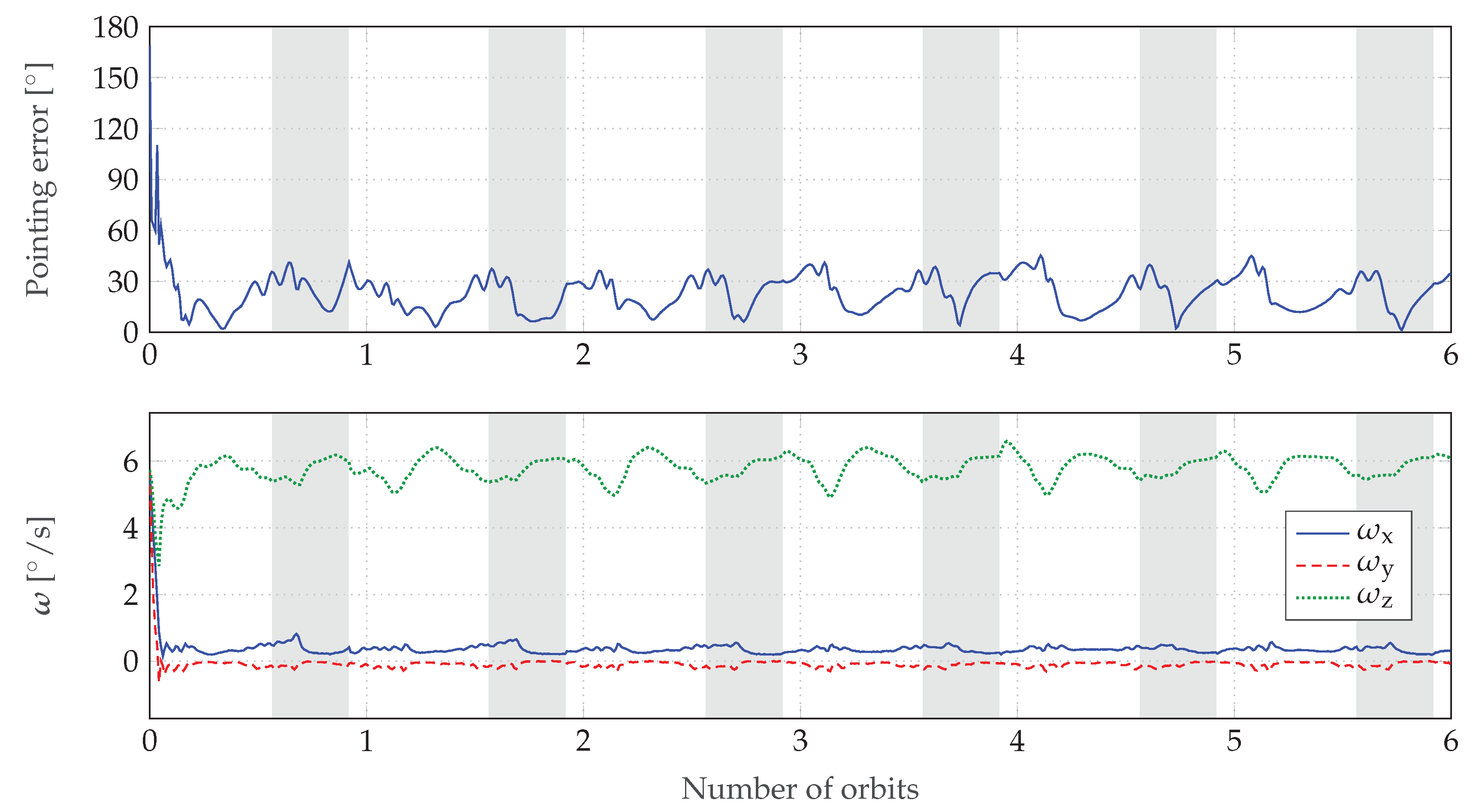
Spinning Sun-Pointing Controller: The non-spinning sun-pointing controller’s tendency to align the desired torque vector with the magnetic field is overcome by adding a spin around the z-axis. The spin of 5.73 °/s stabilizes the pointing vector and enables the ADCS to counter the simulated disturbance torques reliably. The ADCS stays on during eclipse to maintain the spin.
Figure 10 shows the pointing error and angular velocity of the satellite over six orbits simulated with the HIL environment at realistic levels of disturbances. When starting at an initial velocity of 10 °/s, the controller takes ~12
to reduce the pointing error below 10°. The mean pointing error is
with a standard deviation of
. A test run of 16 orbits verifies the long-term stability of the spinning sun-pointing controller and a sensitivity analysis shows that this controller does not become unstable with varying sensor characteristics [
20]. Consequently, spinning sun-pointing replaced non-spinning sun-pointing as the default controller on MOVE-II shortly before freezing all software in preparation for the delivery.
After the software for MOVE-II had been finalized, a Monte Carlo analysis with 100 individual simulation runs was performed to extend the controller’s analysis. This analysis randomly varies the initial attitude and velocity vector.
Table 5 shows the results. We can categorize four different types of behaviors for the spinning sun-pointing controller. Nominal behavior is defined as the convergence to a pointing error below 10° within a time of 25 min. Runs are categorized as slow convergence, when an converging trend is obvious, but the pointing error is still above 10° after 25 min. Two other behaviors are observed, which are highly undesirable. Anti-pointing describes simulation runs where the satellite stabilizes at an attitude pointing away from the sun. Furthermore, in
of the cases, the controller causes an oscillation in attitude, preventing the satellite from stabilizing at the operating point.
3.2. Verification of the Attitude Determination Algorithms
As mentioned in
Section 1, an EKF is implemented to estimate the satellite’s attitude and the gyroscope bias. A singular value decomposition (SVD) method computes the attitude, which can be used as a sanity check of the estimation of the EKF. It also allows to provide an initial estimate for the EKF. Both approaches require environmental models, such as Earth’s magnetic field model, a sun position model, Earth’s rotation, and orbit propagation. The complete attitude determination architecture was verified using the RS, SIL, and HIL approach. As realistic sensor models are required for functional attitude estimation, we skipped the IS approach. We developed the complete attitude determination algorithms in Matlab code to provide a baseline implementation for the firmware code. In the next step, the SIL approach is applied. Therefore, all the required C++ code modules for the attitude estimation are embedded into the Simulink model. The existing C++ code of the EKF was adapted and debugged so that the output is identical to the reference implementation.
We can show that the difference between the Matlab and the C++ estimation output is zero [
24]. In addition, the estimation error of the gyroscopic bias for the Matlab and C++ code converges towards zero. The verified firmware code was implemented on the ADCS Mainpanel for the HIL approach. A couple of test runs are done to investigate the performance on the actual hardware. Utilizing HIL, we could show the main functionality of the EKF, the SVD method, and all required environmental models. The SVD method provided a sufficient initial estimate for the EKF. The environmental models and the modified Julian date computation are verified additionally. The computed output is compared with the environmental models in Simulink. It could be shown that numerical inaccuracies that were expected early in the development phase do not corrupt the performance.
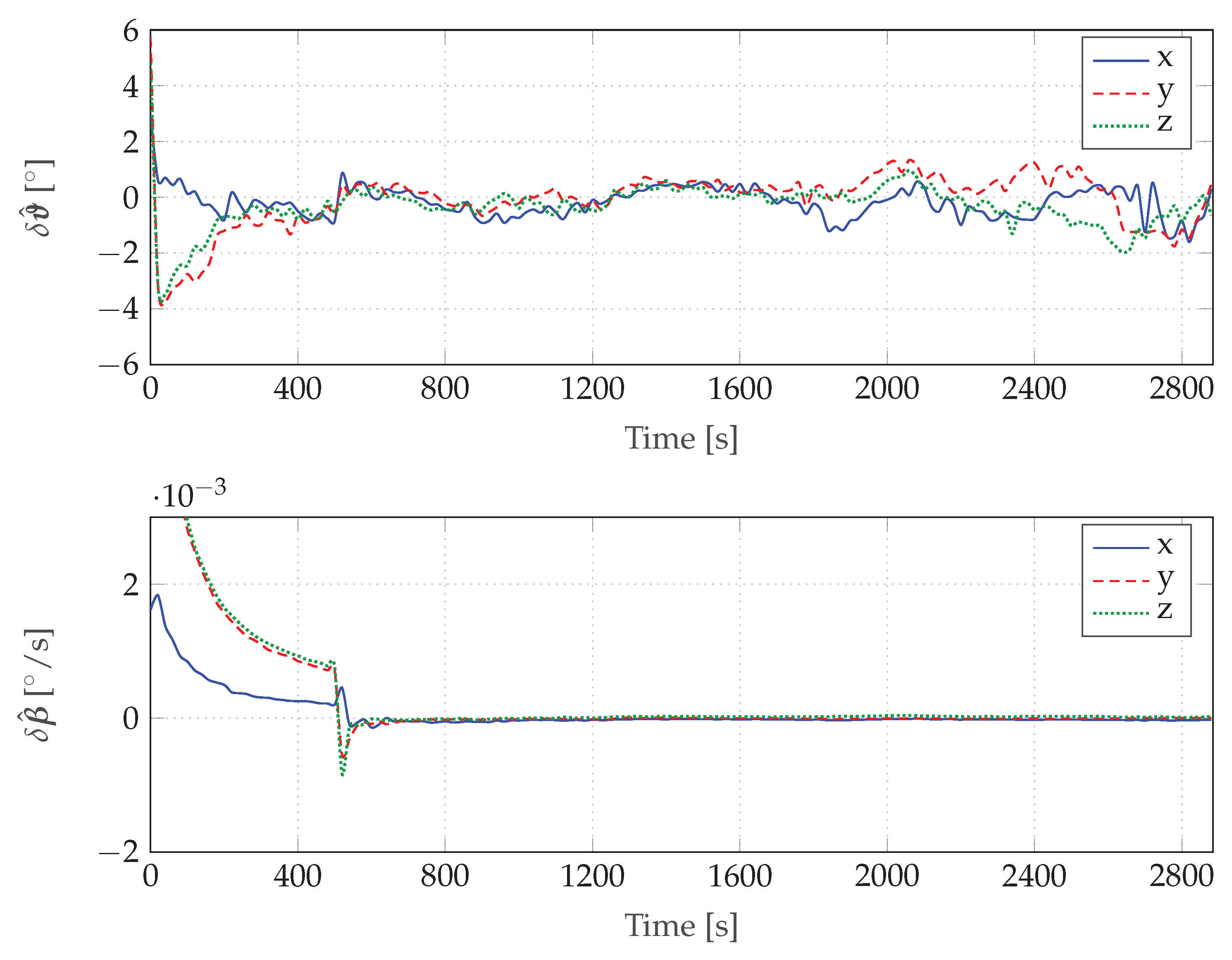
After the EKF initialization procedure during a running simulation, the bias estimate converges as expected from the previous simulation with RS and SIL. The bottom plot of
Figure 11 shows the estimation error of the bias denoted by
converges towards zero very quickly after initialization. This event can be clearly seen as a jump at ~550
. Before the initialization procedure, the bias error converges very slowly.
The upper plot of
Figure 11 shows the attitude estimation error denoted by
. The component are resolved as roll, pitch, and yaw denoted by
x,
y, and
z, respectively.
After 2400
we can see a deterioration of the estimation error, as the sun sensor is not available for the EKF. The estimation errors are not only caused by modeling inaccuracies, but also by the numerical inaccuracies of the EKF computation itself, the reference models, and the Julian date calculation output. In addition, several delays (like network delays) within the HIL framework may affect the estimation errors. A small time shift introduced by the compiling time of the Simulink model, affects the estimation performance. Therefore, we are only able to assess the overall estimation errors including the errors induced by the HIL environment. The overall functionality of the attitude determination architecture implemented on the hardware was previously demonstrated [
24].
In summary, the RS, SIL, and HIL approach provided a powerful tool to verify the attitude determination algorithms in a very structured approach.
3.3. Verification of the EPS and Power Budget
Although the connection between the ADCS interfaces and the Mainpanel carried only digital information, the connection between the solar cells and the EPS carries electrical power. The introduction of
Section 2 already stated that our HIL environment will cover the whole electrical domain, so we need to provide realistic inputs and outputs to the EPS to test it in flight-like conditions and verify the satellite’s power budget. The inputs, i.e., the solar cells, are replaced by the Solar Array Simulator covered in
Section 2.3.2. The outputs, i.e., all consumers of electrical power, are not replaced. The HIL environment includes them as processing hardware. The actuators on the Sidepanels and the Toppanels are one major power sink that are not part of the processing hardware. We connect them in a read-only configuration so they will consume a realistic amount of power but do not disturb the communication (see
Section 2.3.1). This architecture ensures that the HIL environment resembles the electrical power situation onboard the satellite at high precision. Furthermore, the verification is simplified to starting the simulation and observing the state of charge of the battery.
From a power budget perspective, MOVE-II has three basic operational modes: Satellite switched off, Safe Mode, and Nominal Mode. The EPS enters the mode Satellite switched off when the battery voltage drops below 6.2 V, where it turns off all consumers and charges the battery until it reaches a fixed reset voltage and exits this mode. As there are no consumers, and therefore no way to deplete the battery even further, this mode does not need verification. In Safe Mode, the satellite uses as little battery power as possible by powering only CDH, COM, and EPS, but as ADCS is turned off, there is no sun-pointing, which results in reduced available solar power and slower battery charging. In Nominal Mode, the satellite operates normally running CDH, COM, EPS, ADCS, and Payload. It uses more power than in Safe Mode, but thanks to the sun-pointing action of ADCS, the illumination of the solar arrays is optimized, resulting in a higher power income.
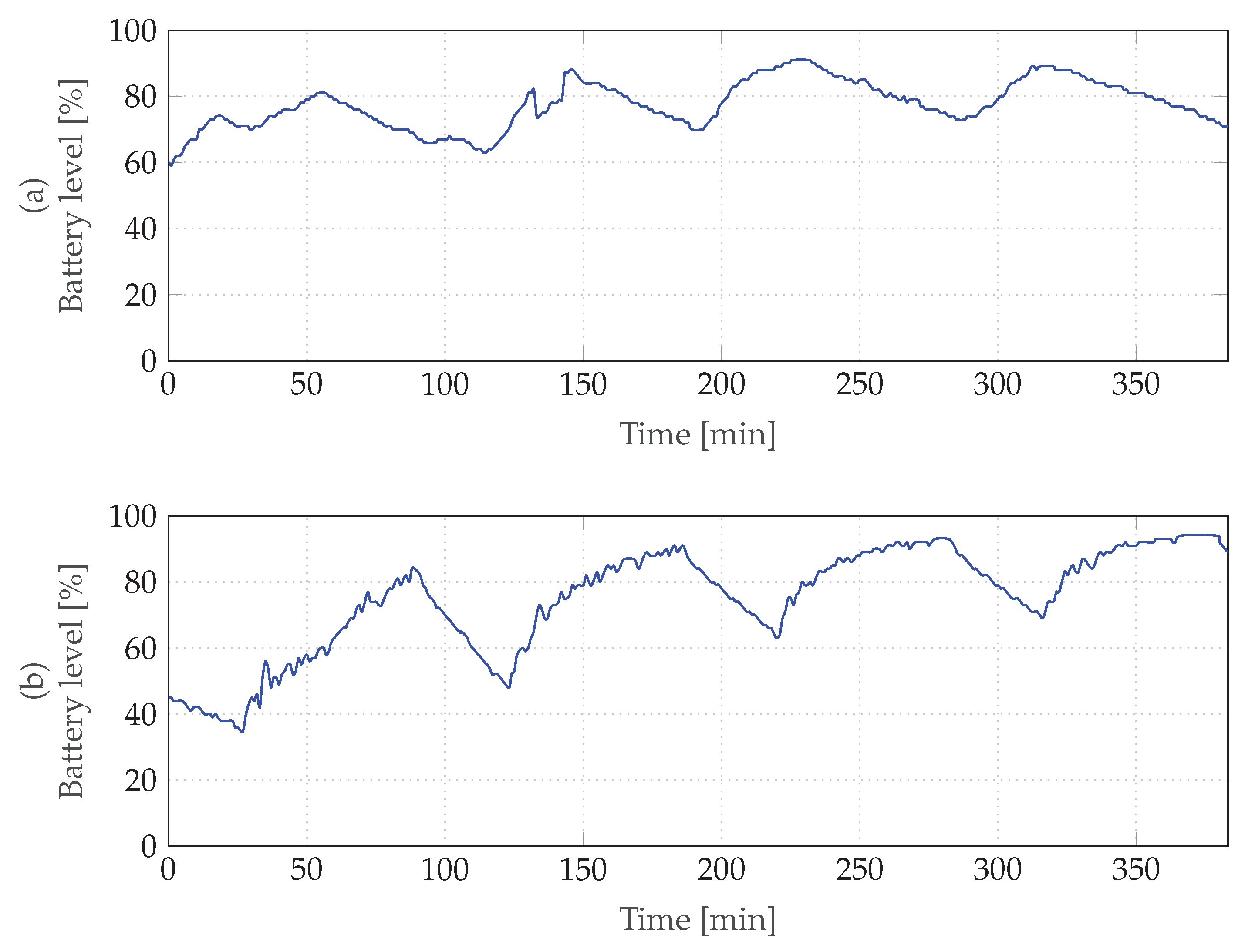
The power budget was verified for
Safe Mode and
Nominal Mode in separate HIL simulations. Both simulations ran for four orbits (approximately 6 and a half hours). The state of charge versus time is plotted for each case in
Figure 12. Periods of sunshine (state of charge increasing) and eclipse (state of charge decreasing) of the four orbits are distinctly recognizable in the plots.
Safe Mode (a) was shown to be power positive by the test, however only with a slight margin, as the overall trend of state of charge is almost flat. On the contrary, the state of charge is clearly increasing in Nominal Mode (b), which verifies a positive power budget for this mode with a safe margin. The little margin of the Safe Mode power budget prompted the team to increase the reset voltage of the Satellite switched off mode so the satellite recharges its batteries until the battery is at ~15% state of charge. Later analysis showed that the satellite would have entered a reboot-loop otherwise when trying to leave the mode Satellite switched off.
The power budget testing with HIL showed that our holistic test approach yields accurate results and more coverage than a completely simulation-based verification. As the MOVE-II team did not have access to the schematics of the EPS, in-depth modeling of this system would have resulted in a poor model anyway. One aspect that our HIL environment completely ignores is the temperature dependency of the battery. With decreasing temperature, the battery efficiency decreases too, thereby reducing the available energy [
25]. The operating temperature of the battery was 25 °C during the power budget tests compared to ~5 °C in orbit. The reduction in efficiency causes the power budget to become negative in
Safe Mode during flight. Consequently, the battery should also be categorized as an interface in a future iteration of the HIL environment and be replaced with a battery simulator that receives the battery temperature from the simulation.
3.4. Benefits during Operator Trainings
During the months preceding MOVE-II’s launch on 3 December 2018, the team organized weekly operator trainings to learn how to analyze and solve problems during short overpasses. The training setup is the HIL environment with the Engineering-Model of MOVE-II as the device under test. For a test, a fault from one of the domains in
Table 6 is injected. Four overpasses with a duration of 10
each are simulated for each test. The team of operators then tries to diagnose the problem and evaluate a possible resolution.
The operators were working in the actual mission control center, visualizing data, and sending commands through the operations interface, that was developed specifically for MOVE-II. The operations interface has a separate database for the engineering model and connects to the experimental ground station in the integration room instead of the roof-mounted ground station. The experimental ground station talked to the satellite transceiver over omnidirectional antennas. The Engineering-Model embedded in the HIL environment as shown in
Figure 5 was sitting on a desk in the integration room.
Augmenting the operator training with a real-time simulation of the spacecraft and its environment adds realism and improves the learning effect for the operators. The most advanced framework for mission simulation and conducting operator trainings known to the authors of this article is the NASA Operational Simulator for Small Satellites (NOS3) [
26]. Although NOS3 replaces the actual hardware with simulated subsystems, our HIL approach covers most of the hardware and all of the software that is used during the actual mission. It includes the stack of subsystems, the ground station PC and SDR, the operations server, and the mission control center.
Using HIL simulations for operator trainings showed several advantages for the mission. The mission controllers gained practical experience with different fault scenarios: they discovered characteristics of the satellite that were not covered by the procedures so far and updated the documentation accordingly. Additionally, knowing that they commanded an actual piece of hardware increased their motivation to resolve the fault scenarios.
3.5. Benefits during Mission Operations
Closely after, the MOVE-II CubeSat was launched on the 3rd of December 2018 while the ADCS was inactive; its angular velocity slowly increased reaching over 500 °/s. The most probable reason for this behavior is a magnetic dipole created by the solar cell wiring [
19].
The ADCS is not designed to work under high angular velocities. If the velocity rises above a few hundred degrees per second, the delay between measurement and actuation will cause instability. This section gives an overview on the analysis carried out to understand the ADCS behavior in orbit and detumble the satellite successfully.
We can show that the average decrease of the angular velocity that the detumbling controller produces is proportional to
where
is the angular velocity of the satellite,
is the length of the actuation interval,
T is the time between actuations (thus,
is the controller’s duty cycle), and
is the time elapsed between the measurement of
(the time derivative of the magnetic field of the Earth measured in the body frame, which is used to compute the magnetic control moment) and the center of the actuation interval. Note that the B-dot detumbling algorithm keeps the generated magnetic control moment constant over the whole actuation interval
.
From Equation (
2), we can derive the stable regions of
. If Equation (
2) is positive, the satellite’s angular velocity decreases. The function’s first root is given by
For
the controller is able to reduce the angular velocity. Therefore,
represents the boundary angular velocity of the stable range. For the computation of
, the processing delays given in
Table 7 must be taken into account.
The B-dot detumbling algorithm derives from a linear fit over the last five measurements, which are obtained every . Therefore, the estimated value is valid at the center of this measurement interval, and this method for computing results in a measurement delay is added to . The calculation and the command transfer to the actuators take 35 . Furthermore, as the commanded current stays constant over the whole actuation period, an extra delay must be added to .
The spinning sun-pointing controller behaves like a detumbling controller for high angular velocities. Therefore, its stability was analyzed since it could also be used for detumbling the satellite. In contrast to the detumbling controller, it does not use a buffer for measurements, thus the 125 delay is not present in this controller. However, the processing delay and the actuation period are significantly longer, so its is longer than the B-dot’s overall delay.
Using the SIL approach, it is possible to characterize the behavior of the controllers for various initial angular velocities. Therefore, several Monte Carlo simulation runs were conducted. The initial angular velocity was randomly initialized for each test run. The average difference in the norm of the angular velocity that the controllers achieved after a fixed amount of simulation time, denoted by
, was computed.
Figure 13 shows the different stability and instability ranges of both the detumbling controller and the sun-pointing controller. The controller is able to reduce the angular velocity after simulation run time within the stability region with
. We can show that the curves obtained by the theoretical considerations using Equation (
2) can be verified by the simulation test runs.
As the controllers’ gains can be changed from ground, it is possible to invert their signs in order to make the unstable ranges stable (but also the stable ranges unstable). Thus, considering the satellite’s current angular velocity, we can choose between sun-pointing and detumbling controllers, with or without inverted gain, to make the algorithm stable for a given angular velocity. Through iterations of this process over several months, we have been able to detumble MOVE-II from an initial angular velocity value beyond the algorithms’ maximum stable angular velocities. The SIL approach proved to be useful for troubleshooting this situation and for verifying the theoretical models.
3.6. Verification of New Software
The HIL environment provides the possibility to test new algorithms that can be uploaded to the satellite later on. This section presents new attitude control algorithms that have been designed and tested in the HIL environment. We apply different simulation approaches as summarized in
Table 4. The IS and RS approaches are used to design the controllers, whereas the SIL approach helps to implement and verify the C++ code. Finally, the HIL approach verifies the code implemented in hardware. After verification, the presented controllers were included in MOVE-IIb’s flight software.
3.6.1. Evaluating New Control Strategies for Sun-Pointing
The evaluation of the spinning sun-pointing controller in
Section 3.1 makes confirms that there is still potential for more accurate and more reliable controllers. The following sections present the verification of one state-feedback controller, namely, the extended LQR controller, and one Lyapunov-based controller, namely, the Delta-H controller.
During development, the controller of the JC2Sat mission [
27] and the modularly constructed controller proposed in [
28] were considered and analyzed, too. However, they did not show promising result in the RS setup for MOVE-II. Detailed analysis of these controllers can be found in [
23].
Extended LQR Controller: With the HIL simulation, we could identify the shortcomings of the spinning sun-pointing controller stated in
Section 3.1. After analyzing the spinning sun-pointing controller’s shortcomings, a new controller was developed to improve the pointing performance. The gain is calculated using the LQR algorithm [
29], especially penalizing a deviation in the pointing error. This leads to a faster convergence of the pointing error. The detailed description of this controller can be found in [
23] (pp. 39–49).
Figure 14 compares the results of a Monte Carlo simulation in SIL with the spinning sun-pointing controller (a) and the extended LQR controller (b). In total, 100 runs are performed for every controller. Five successful runs are shown in the figure. A Monte Carlo run is considered a success if the pointing error converges below a threshold of
within 0.26 orbits. It is obvious that, on average, the extended LQR controller converges faster than the spinning sun-pointing controller. When analyzing all runs of the Monte Carlo simulation,
of the spinning sun-pointing controller are successful and
of the extended LQR controller are successful. The final pointing errors are
and
, respectively. Thus, SIL helps to compare these two controllers and make an estimate, which of them performs better in space.
Delta-H Controller: As
Section 3.1 shows, the spinning sun-pointing controller only shows nominal behavior in
of the cases. The issue of limited convergence towards the operation point is a possible characteristic of linearized controllers if the system equations are nonlinear. To overcome this issue, we implemented and tested the Delta-H controller, whose nonlinear control law is based on a Lyapunov function. The basic idea of this controller is first proposed in [
30] and then extended for global convergence in [
31].
The nonlinear control law ensures global convergence to the desired attitude from any initial attitude and angular velocity. Consequently, the success rate of the Delta-H controller in a SIL Monte Carlo simulation is
, as
Figure 15 demonstrates. In a HIL simulation, the implementation of the Delta-H controller could be verified successfully on the flight hardware. As the Delta-H controller achieves a similar pointing accuracy as the spinning sun-pointing controller [
23], it was included in MOVE-IIb’s flight software.
3.6.2. Fast-Detumbling Algorithm
Based on the stability analysis performed in
Section 3.5, a modified version of the detumbling algorithm was implemented (fast-B-dot algorithm), which in theory would have a considerably larger stable
range.
This control algorithm was developed based on the experience with MOVE-II and implemented in time for adding it into the MOVE-IIb firmware before the launch. This provides an additional option for detumbling the satellite in situations similar to those experienced with MOVE-II, and allows detumbling without having to switch between the inverted or non-inverted sun-pointing and detumbling control algorithms.
The main idea behind the fast-B-dot algorithm is to measure the satellite’s angular velocity and use it to extrapolate the value of the measured magnetic field of the Earth to the center of the actuation interval, so as to decrease the value of
(see Equation (
2)). Afterwards, the angular velocity is used once again to estimate the value of the time derivative of the magnetic field based on the previous extrapolation, instead of using a buffer as in the original detumbling algorithm. These modifications, which are implemented with a single formula, eliminate both the measurement delay and the extra
that needed to be considered before. The estimated value of the processing delay is also considered for the extrapolation. As the timing of the algorithm defines the stability ranges, it was implemented in a way that its timing values (
,
T, and the extrapolation time) can be reconfigured from ground.
Without extrapolation, it will always be the case that
, and then, based on Equation (
3),
With the extrapolation, a value of
is achieved and, as
, then
Note that the value of is highly sensitive to the value of when , but as long as the value of is decreased with respect to the value of of the unmodified detumbling algorithm, the stable range will be extended, and if is achieved, then the value of will only depend on the length of the actuation interval .
As the delays of the HIL setup would affect the behavior of the fast-B-dot algorithm, a SIL simulation was performed to verify that the algorithm implementation was working properly and as expected. The same simulations that were performed for the stability analysis were performed once again but with the addition of the implementation of the fast-B-dot algorithm. The fast-B-dot controller’s timing values are given in
Table 8.
Figure 16 shows the stability regions of the fast-B-dot controller compared to the default B-dot detumbling and spinning sun-pointing controller. These curves have been verified by Monte Carlo simulations utilizing the SIL approach. The timing values of the detumbling and sun-pointing controllers can be found in
Table 7 for reference.
The SIL approach allowed us to verify that the implementation of the algorithm was working properly and, combined with other testing methods we used, it allowed us to develop and verify the modified ADCS firmware in time for uploading it onto MOVE-IIb.
4. Conclusions
The simulation environment presented in this article helped us to verify MOVE-II’s flight software with a strong focus on ADCS. The verification of the attitude control algorithms mentioned in
Section 3.1 showed how our simulation approach helped the developers to discover and resolve instabilities efficiently. The verification of the power budget presented in
Section 3.3 included the maximum power point trackers, all voltage regulators, the battery, and all power consumers in hardware. Thus, we avoided the effort of modeling these nonlinear systems. The inclusion of the electric domain in the design of the HIL environment resulted in accurate measurements of the satellite’s power budget in the most important mission phases. Also, without the adjustments to the EPS’s reset voltage prompted by the power budget verification, MOVE-II would have ended up in a reboot loop leading to a failed mission. The simulation environment was easy to extend and combine with the MOVE-II ground station enabling the realistic operator trainings mentioned in
Section 3.4, and it helped to analyze the high spin rate of MOVE-II and select the best strategy to detumble the satellite as discussed in
Section 3.5. After the MOVE-II launch, algorithms that could be successfully verified in the HIL environment were implemented on the next satellite MOVE-IIb, as mentioned in
Section 3.6. We see HIL verification as an efficient way for new developers to prove correct functionality of the software in short time.
In summary, the work with this testing environment shows how we can enhance the reliability of CubeSats through system-level tests. Future work on the HIL environment and its application to earlier stages of satellite development will help to have a more holistic approach to CubeSat testing on-ground. Despite the current limitations of the simulation environment, the test approach carried out on MOVE-II had clear benefits for the mission and helped to ensure a reliable satellite operating in space.
Future work will include reworking the current implementation of the hardware interfaces. The universal interface node (UIN) mentioned in
Section 2.3.4 is both faster and more flexible than the previous hardware interfaces. It shall be primarily used in future missions. Despite the development of MOVE-II and MOVE-IIb being finished, work on the HIL environment is ongoing to improve the thermal model and the channel simulator, so as to improve the operator trainings. As all tests can be fully automated, the environment is suitable for inclusion in a continuous deployment workflow where code changes trigger automatic tests on the hardware.
We think that a HIL environment containing the processing hardware of all subsystems and covering the domains of digital sensor signals and electric power is a good testing solution for every CubeSat mission, especially if the power income depends on the satellite’s attitude. We see it as a scalable and expandable test approach with relatively little development effort, low cost, and high hardware coverage.

 ,
, 


