In-Flight Aircraft Trajectory Optimization within Corridors Defined by Ensemble Weather Forecasts


Chair of Air Transport Technology and Logistics, Technische Universität Dresden, 01069 Dresden, Germany
*
Author to whom correspondence should be addressed.
§
These authors contributed equally to this work.
Aerospace 2020, 7(10), 144; https://doi.org/10.3390/aerospace7100144
Submission received: 28 July 2020
/
Revised: 4 September 2020
/
Accepted: 29 September 2020
/
Published: 1 October 2020
(This article belongs to the Collection Air Transportation—Operations and Management)
Abstract
:Today, each flight is filed as a static route not later than one hour before departure. From there on, changes of the lateral route initiated by the pilot are only possible with air traffic control clearance and in the minority. Thus, the initially optimized trajectory of the flight plan is flown, although the optimization may already be based upon outdated weather data at take-off. Global weather data as those modeled by the Global Forecast System do, however, contain hints on forecast uncertainties itself, which is quantified by considering so-called ensemble forecast data. In this study, the variability in these weather parameter uncertainties is analyzed, before the trajectory optimization model TOMATO is applied to single trajectories considering the previously quantified uncertainties. TOMATO generates, based on the set of input data as provided by the ensembles, a 3D corridor encasing all resulting optimized trajectories. Assuming that this corridor is filed in addition to the initial flight plan, the optimum trajectory can be updated even during flight, as soon as updated weather forecasts are available. In return and as a compromise, flights would have to stay within the corridor to provide planning stability for Air Traffic Management compared to full free in-flight optimization. Although the corridor restricts the re-optimized trajectory, fuel savings of up to 1.1%, compared to the initially filed flight, could be shown.
1. Motivation and Introduction
Today, aircraft operators are claiming for a high degree of freedom in flight planning to maximize their cost-saving potential by choosing optimum altitudes and cruising speeds. On the other hand, the Air Traffic Management (ATM) requires reliable predictions of aircraft 4D positions to maintain safe and orderly traffic flows at any time. This work extends the typical flight-planning problem by a periodical re-optimization of trajectories during flight with updated weather forecasts. For increased predictability in ATM, the so-called Corridor of Optimization (CoO) is introduced as an agreed solution space for trajectory re-planning with Air Traffic Control (ATC), which is requested once before departure. Since wind is a major source of flight plan instability even when in-flight, the CoO is also determined by such uncertainty. Consequently, the accuracy of weather data is analyzed before the CoO is calculated by use of the Global Ensemble Forecast System (GEFS) system with 21 ensembles for each forecast. For typical weather forecasts in August 2019 and January 2020, savings in fuel and time are assessed for flights with in-flight re-optimization inside a CoO defined before departure, assuming that ATM (basically ATC) would agree on change requests from the flight deck in time.
In civil air traffic, each trajectory following Instrument Flight Rules has to comply with various capacity constraints, such as sector load laid down by the Air Traffic Flow Management (ATFM) units (e.g., the Network Manager in Europe, cf. ICAO Doc. 4444 PANS-ATM [1]) or lateral and vertical separation of aircraft (PBN/RNP) [2]. The therefore required flight plan is composed of waypoints, cruising speeds, and altitudes. It is used for airspace demand-to-capacity balancing and is calculated one hour before scheduled off block time at the latest, based on the most recent weather data. After submission of the flight plan, i.e., in-flight, changes cannot be considered, and the trajectory is flown as filed, except for safety reasons [3].
The flight planning is based on atmospheric conditions, which are often modeled as deterministic in nature, e.g., based on the commonly used Global Forecast System (GFS). Since we know well about the impact of various uncertainty sources in aviation on to the trajectory execution [4], the wind speed and direction, with increasing uncertainty over the look-ahead time, is the most relevant one (see Figure 1). Due to permanent fluctuation of the atmospheric conditions, the temporal optimum trajectory differs most likely from the initially filed one, causing extra fuel and/or flight time. In addition, the unsteady atmospheric conditions lead to an uncertain arrival time and affect the ATM process as well. Therefore, the integration of forecast uncertainties may benefit both the flight efficiency as well as the ATM planning stability.
Cyclic weather updates and re-optimization of the trajectory during the flight provide the opportunity for more efficient trajectories [5]. Current ATM infrastructure projects aim to establish less restrictive flight planning capabilities through Functional Airspace Blocks and Free Route Airspaces. For a comprehensive overview, see [3]. In the near future, free flight initiatives focus on providing the capability to react on changing flight conditions even during flight, which decrease the predictability of the trajectory drastically. Furthermore, a Trajectory Option Set (TOS) has recently been introduced in the U.S., which enables automated negotiation of trajectories with the U.S. traffic flow management system. TOS significantly increases flexibility in the implementation of efficient routes and is also considered for in-flight optimization in the future [6]. By nature, uncertainties should not conclude in a single specific route but rather in a bunch of solutions, forming a solution space. Here, the CoO contains the optimum trajectory with a given probability and, as the weather forecast quality worsens with increasing flight time (Figure 1), the aircraft should be permitted to choose its real optimum during flight within the CoO.
1.1. Trajectory Optimization with Forecast Uncertainties
Various approaches exist to determine a robust, optimized trajectory in the flight planning phase, i.e., before departure of the actual flight. Li et al. [7] present a dynamic optimal control problem where stochastic equations are transferred to equivalent deterministic differential equations. However, uncertainties are represented by one variable, and large-scale problems are hard to compute. Arribas et al. [8] present a robust optimal control methodology to calculate trajectories in the presence of weather uncertainties. In [9], they examine the influence of wind forecast accuracy on the robust trajectory and investigate cubic interpolation of wind. Legrand et al. [10] provide an approach by gridding the world, applying a Bellman shortest path algorithm for each forecast ensemble and identifying the most robust trajectory using cluster analysis. Two years later, Franco et al. [11] generated optimized lateral paths for a transatlantic flight based on weather uncertainties derived from ensemble weather forecasts. There, the optimal path was calculated with a Mixed-Integer Linear Programming approach that provides a trade-off between minimum flight time and minimum arrival time uncertainty. In [12], the same team estimates the probabilistic fuel consumption due to weather uncertainty with a simplified flight performance model. Cheung et al. [13] made recommendations for decision-making at robust trajectories in pre-departure planning. Lindner et al. [14] calculated a robust trajectory using the optimization core of TOolchain for Multi-criteria Aircraft Trajectory Optimization (TOMATO), which provides various target functions to optimize trajectories in a free route airspace [15,16]. However, those studies determine a trajectory robust to uncertainties by choosing the flight profile with less fuel consumption for all ensembles or low standard deviation of uncertainties along the path.
1.2. In-Flight Re-Optimization of Trajectories
In addition to robust pre-flight optimization, uncertainties in the weather forecast can be addressed during flight, whenever updated weather data are available. The NASA TASAR combines lateral and vertical trajectory recalculation in case of convective weather while considering surrounding air traffic [17]. Lindner et al. [5] showed that periodical weather updates and a subsequent re-optimized lateral trajectory saves fuel and reduces costs by approximately 1%. Therein, the pre-flight trajectory was calculated based on the latest available GFS cycle, then hourly weather forecasts from the GFS were assumed as weather updates to re-optimize the trajectory from the aircraft position. However, this approach assumed weather forecasts to be static, which overestimates the optimization potential of the re-optimization. In [14], the concept was improved by using dynamic weather forecasts and the hourly updating weather model Rapid Refresh (RAP). Recently, in 2019, a test flight with the Boeing EcoDemonstrator proved the feasibility of in-flight-optimized trajectories with TOMATO.
Re-optimization during flight may induce deviations from the initially filed flight plan, which need to be covered for ATM purposes. ICAO’s Performance Based Navigation (PBN) Manual [2] defines areas of Required Navigation Performance (RNP) as a safety buffer for deviations from routes to cope with navigational and operational errors. In this study, this idea is transformed into the CoO as an area for negotiating optimization during flight. Inside the CoO, flights are permitted to adjust their profile on updated weather information, while the ATM-driven need for a predictable flight behavior is still met by negotiating the extent of the CoO before departure. In this work, we assess the size and the shape of generated CoO and its fuel-saving potential on the actual optimal trajectory because aircraft must not leave the CoO.
1.3. Focus and Structure of the Document
We provide a case study to calculate the potential of re-optimization of flights during flight operation in order to react to uncertainties in pre-departure weather forecasts. For this purpose, we determine hard boundaries as optimization constraints from the quantified uncertainties of the weather forecast before departure. Once filed, those constraints shall not be adapted during flight. Within these boundaries, the re-optimization from the current aircraft position can then take place, whenever a new weather forecast is available. These results are then compared with unconstrained in-flight optimizations to quantify possible losses due to the constraints. The optimization potential of a CoO-based re-planning of trajectories is evaluated from the single flight perspective only. The implementation of this concept might require changes to the ATM procedures or might even reduce the airspace capacity. Although it is out of the scope of this paper, we discuss these possible issues in the outlook.
Our contribution is structured as follows. After the introduction and literature review in the fields of trajectory optimization, trajectory uncertainties and in-flight re-optimization, we discuss uncertainties quantified in weather forecasts and compare them with measured data from aircraft in Section 2. In Section 3, we introduce the methodology for the design and evaluation of the CoO, an optimization space for trajectories. Section 4 applies this optimization for a daily flight for a summer and winter month. Finally, our work is summarized and an outlook is provided in Section 5.
2. Reasons for a Required Modification of the Filed Flight Plan
The optimum 4D single trajectory strongly depends on the current weather conditions. In particular, wind speed and wind direction lead to a deviation between the ground-based and the aerodynamic coordinate system of the aircraft movement [3,5]. Hence, the dispatcher optimizes the trajectory considering predicted atmospheric conditions. For this, theoretically, three different sources of weather information are available.
First, surrounding aircraft are measuring the state parameters of the atmosphere (pressure p and temperature T) and are calculating wind direction and wind speed. In the Aircraft Meteorological Data Relay (AMDAR) system, these collected data are transmitted directly by Very High Frequency (VHF) communication via the Aircraft Communications Addressing and Reporting System (ACARS) or by a satellite link to a receiving station on the ground. After the data are collected centrally, it undergoes intensive quality control and post-processing before being distributed to the airlines, weather services, and other users [18]. With the help of these data, a significantly better temporal and spatial resolution of vertical soundings of the atmosphere is available, especially in areas with increased air traffic.
Second, numerical weather models use AMDAR and radiosonde data to update continuous calculations of the current global atmospheric state and forecasts with different time horizons. Every six hours, the National Weather Service (NWS) of the National Oceanic and Atmospheric Administration (NOAA) uses the Global Data Assimilation System (GDAS) and GFS to forecast the global weather for the next 384 h and publishes a data set for each hour. Furthermore, the numerical weather forecast model RAP provides hourly weather forecasts at short range with a small spatial resolution of 13 km (8 NM) and 50 vertical layers up to a 10 hPa level of the atmosphere, which covers the United States. RAP is also performed by the NOAA National Centers for Environmental Prediction (NCEP) and is fed by the GFS with the boundary conditions. Every hour, the model provides for 18 h of forecast output.
Third, predictions from the so-called GEFS are carried out. Due to the chaotic nature of the weather, a slight change in the initial data can lead to a complete change in the forecast in many cases, especially for medium and long-term forecasts. Therefore, in addition to the so-called main run, in which the computers use the actual measured values, 20 further runs are carried out, in which slightly changed data and a somewhat coarser resolution of the model grid points are used. The NCEP provides the GEFS, which attempts to quantify the amount of uncertainty in a GFS forecast [19]. The results of these runs are compared in ensembles. If the results for a period are similar to the forecast, it indicates that the forecast for this period is relatively reliable. The initial disturbances for the ensemble members are generated using random (stochastic) disturbance, disturbance of the assimilated observations, disturbance in the direction of greatest disturbance sensitivity with so-called singular vectors or re-scaling of the divergence of previous forecasts (breeding). More recently, the uncertainty in the parameter settings during model integration by disturbance of the computational variables contained therein has also been taken into account (stochastic model physics and multiphysics). Global ensemble models are developed, for example, at the European Center for Medium-Range Weather Forecasts (ECMWF), UK-Metoffice, the NCEP in the USA and Canada, and by Météo France.
Differences among the AMDAR measurements, the model output, and the forecasts are subject to strong fluctuations and represent the solution space in which the in-flight optimization should take place.
2.1. Uncertainties in Weather Forecasts and Measurements
The variability in weather data which should be expected and considered in the CoO design corresponds to the dynamics in weather data. This time behavior is reflected in the prediction accuracy of the climate model (GFS). In the United States, differences in wind speed between a six-hour GFS forecast and the corresponding GFS model output from the new cycle (six hours after the forecast has been calculated) amount to small values between 1 and 5 m s, rarely up to 10 m s (see Figure 2). However, it is not possible to directly derive a high model prediction accuracy from this, since, due to the spatial resolution of even 0.25°, there is a risk that local dynamic effects cannot be mapped.
The similarity between the mean of 21 six-hour GEFS ensemble forecasts, compared to the next GFS model output (cycle), quantifies the reliability of the ensemble forecast. This comparison, as shown in Figure 3, yields smaller differences (in terms of Mean absolute errors, MAE) of MAE = m s, compared to the six-hour GFS forecast (Figure 2) of MAE = 3 m s in wind speed on 29 January 2020. Here, wind speed denotes the vector length, defined by the horizontal wind components u and v. Similar differences occurred on 31 January 2020 (not shown). This can be judged as an additional indicator of a high prediction accuracy or low dynamics in the model.
The standard deviation of the 21 six-hour GEFS ensemble forecasts gives another hint on the reliability of the GFS forecast and directly influences the size of the CoO. On 29 January, the standard deviation was significantly smaller in the western part of the United States than two days later on 31 January (see Figure 4). Hence, a smaller CoO is to be expected for 29 January.
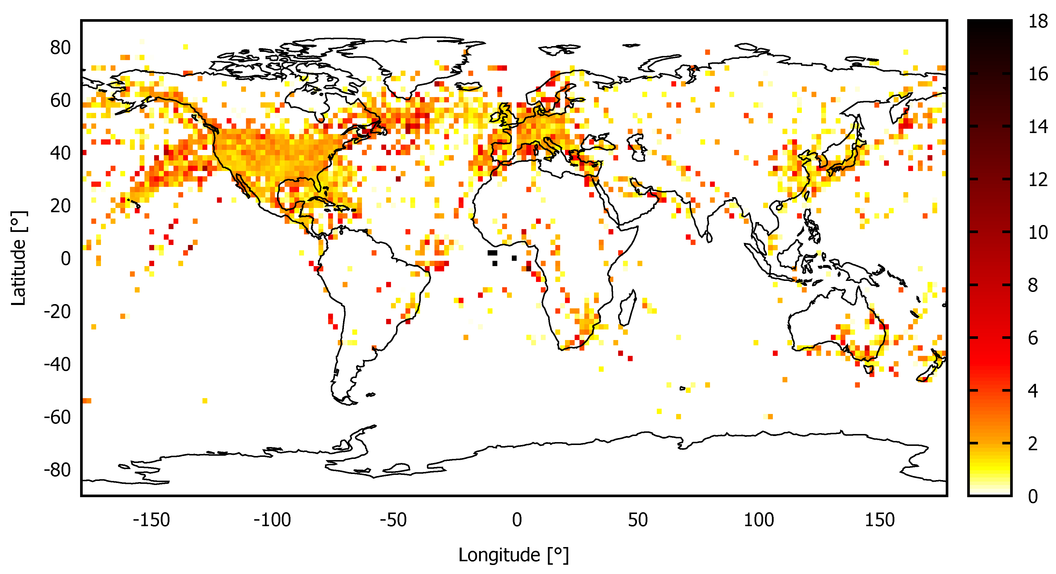
The prediction uncertainty shown in Figure 3 is smaller in the northern hemisphere than in the southern hemisphere (Figure 3). Specifically, in the United States, the prediction is very good. This gain in precision is the result of highly frequent measurements taken by aircraft within the AMDAR concept. Together with the even-more locally limited radiosonde measurements, these data represent reality best. Aircraft type and altitude-specific measurement errors in temperature have been quantified around 1 K [20]. Mean differences in wind speed between these local measurements and the closest global GFS model output are approximately half of the differences between GEFS and GFS (compare Figure 3 with Figure 5).
From the analyses in Section 2.1, it follows that the prediction of the GFS model is very close to the closest GFS output (1 to 3 m s) and independent of the prediction model. Furthermore, the GFS model output is very similar to the measurements taken by aircraft and, therefore, can be considered as realistic. The scattering of the 21 six-hour GEFS ensemble forecasts, however, is twice as large as the prediction error and therefore should be used for the CoO design.
3. Trajectory Optimization Using Ensemble Forecasts
3.1. Pre-Flight Trajectory Optimization
To optimize aircraft trajectories and quantify the operational costs and the environmental impact, we use TOMATO with a deterministic weather forecast. TOMATO is based on three core modules, which iteratively improve the 4D-trajectory towards the optimization target function. For a comprehensive overview, see [3,5,15,16]. Each iteration consists of the following three steps:
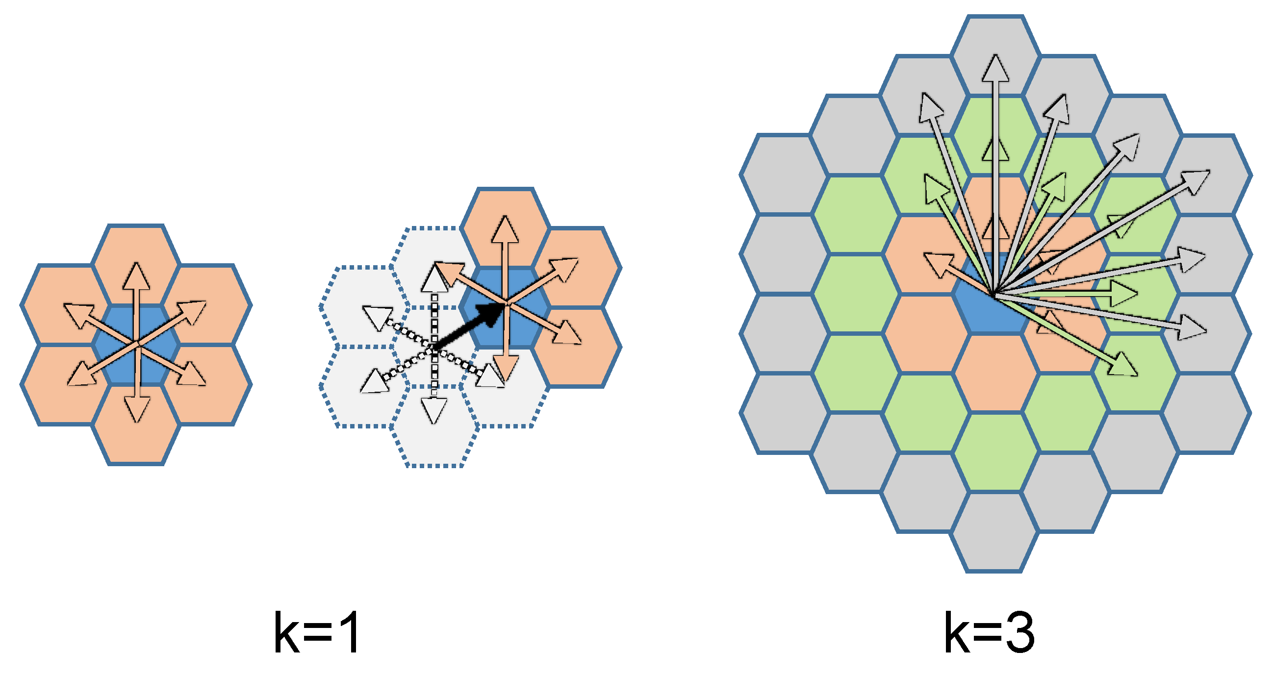
In the first step, an A-Star shortest path algorithm finds the cost-optimal flight path for a set of cruising altitudes between FL 310 and FL 400 considering the imported weather forecasts. The path is generated using a grid either with a variable spatial resolution, an Aeronautical Information Regulation and Control (AIRAC) cycle, or any other geospatial indexing system. In this work, the JAVA implementation of the hierarchical geospatial indexing system from Uber is used to grid the world (resolution step 5: equidistant spatial resolution of ≈15 km and neighbor rings) [21]. This grid uses hexagons, where each center of a hexagon is available for path finding. The left side of Figure 6 shows the path search with neighboring ring in two steps. By increasing k (right part, only one step), significantly more hexagons are included in the path search (). The higher the k, the larger the set of possible direction changes available while the computational effort increases at the same time. It does not allow for choosing an arbitrary direction change, but the options are significantly higher compared to a common global grid (i.e., a discrete spherical coordinate system), especially in the case of a small resolution for the hexagons.
In the second step, the flight performance model COmpromized Aircraft performance model with Limited Accuracy (COALA) determines the climb, cruise, and descent profile for the given path and altitude combination and specific aircraft and engine combination [22,23]. COALA analytically solves the equation of motion considering the required manoeuvre-specific forces of acceleration for each time step (1 s). The flight altitude is variable and not dependent on the flight level system. The altitude is optimized by an iterative variation of different cruise pressures so that overall operating costs are minimized.
In the third step, the assessment module calculates the total operating costs, flight time, fuel burn, and emissions of the 4D-trajectory. Herein, the aggregated optimization parameters of average cost per second, cruising speed, and the fuel on board are calculated, which are used for successive iterations until the target function converges.
3.2. Corridor of Optimization in Flight Planning
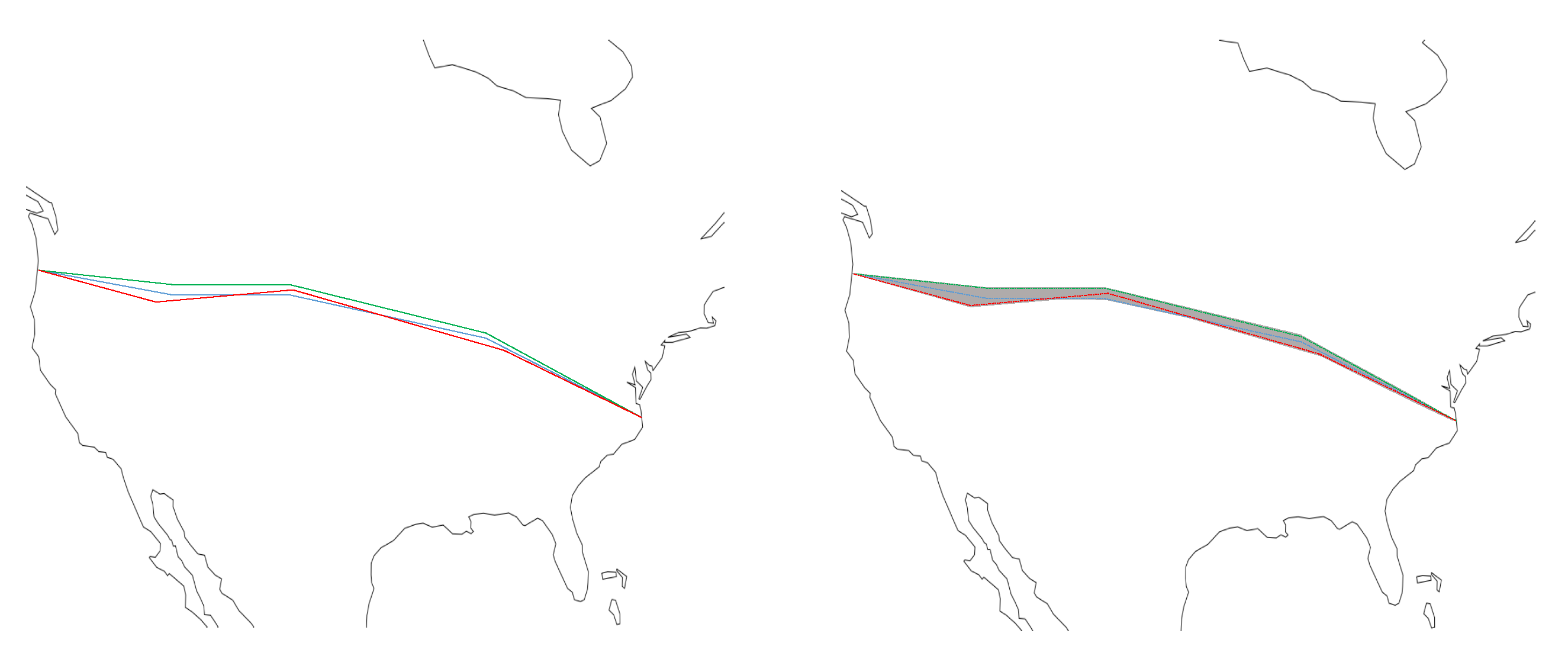
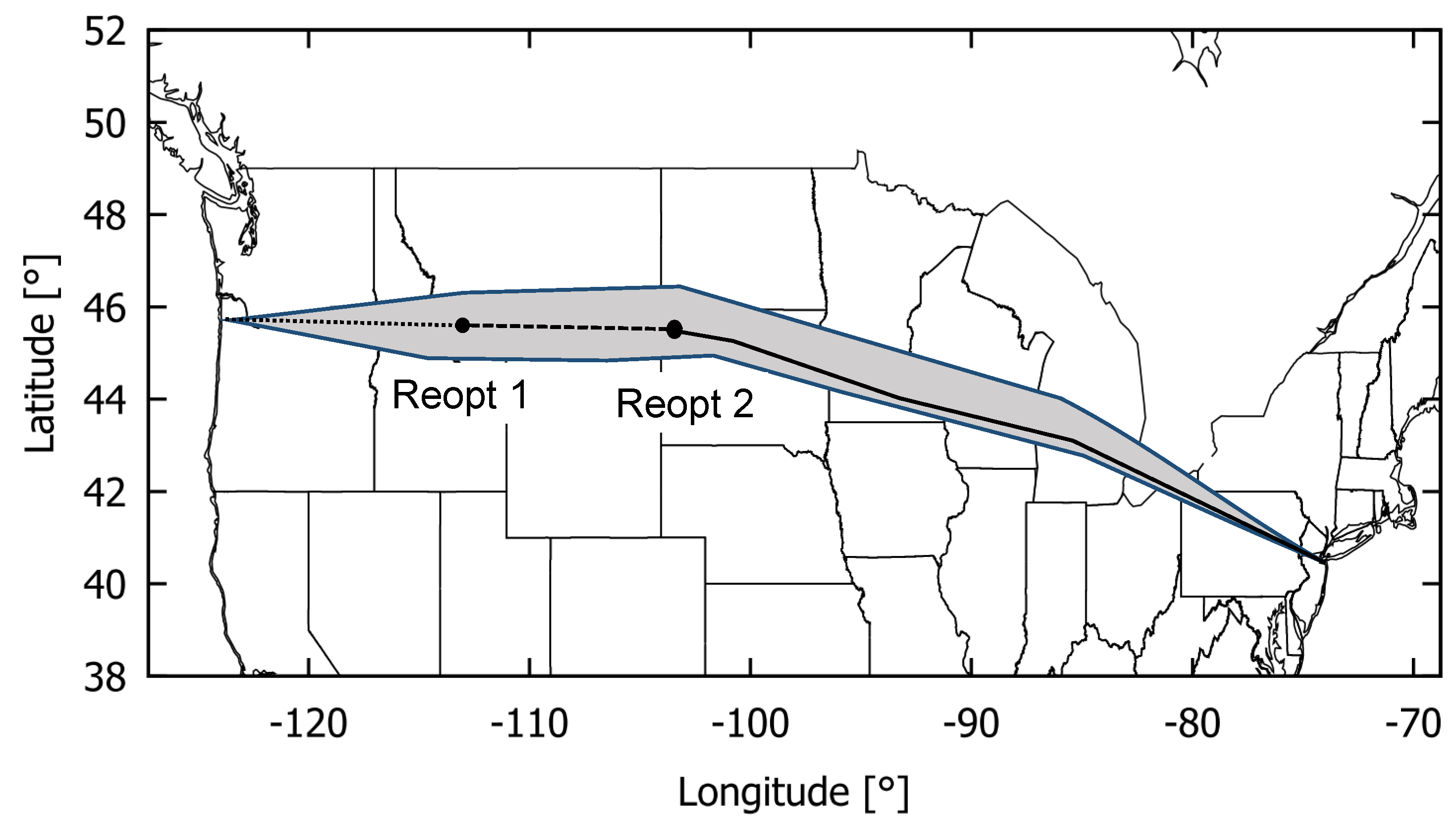
The CoO is calculated using a set of 21 deterministic weather forecast ensembles from GEFS, published parallel to the GFS forecast cycle. For each forecast ensemble, TOMATO calculates an optimal ensemble trajectory as described in Section 3.1. The crossed waypoints of each profile are then jointly merged into an encasing concave polygon hull describing the trajectory solution space as CoO (see Figure 7). The 2D hull is calculated as an alpha shape using the Python alphashape library [24] with . The third dimension, altitude, is evaluated for the resulting optimum cruising altitudes of each ensemble trajectory. For the following in-flight optimizations, the CoO is handled as a restriction, where the borders must not be crossed. It must be ensured that departure and destination are within the CoO. To guarantee that the entire hull describes a valid solution space, it is enlarged slightly with a lateral buffer of 1 NM, (see Figure 8). Since this buffer is smaller than the resolution of the world grid, the CoO is not violated during path finding.
During in-flight optimization, it is improbable to leave the CoO, since expected strong deviations in the weather data are already taken into account. Thus, the flight remains predictable at least within the given area, when filing the CoO to the ATM stakeholders. To further increase predictability, the CoO can be narrowed up to a single reference trajectory by successively eliminating the most penalizing ensemble trajectory or by user-defined limitations (e.g., prohibited airspaces). Although the eliminated forecasts are not necessarily less probable than the remaining forecasts, the dimension of the filed CoO may be reduced by sacrificing some potential for optimization, if capacity considerations require a more precise trajectory. Furthermore, the elimination process could also be oriented on the successive reduction of arrival time uncertainty from the ATM view.
In addition to the CoO, an initial trajectory must be defined to fulfill today’s ATM concept and to provide an ATC and operational flight plan. Although common methods can be used to identify specific robust trajectories (e.g., trajectory with the lowest sum of total operating costs in each ensemble forecast, as pointed out in Section 1.1), this work follows the current flight planning procedure, as it defines the reference trajectory as calculated in deterministic weather forecasts (here: GFS. However, this trajectory is neither necessarily the optimum for each weather ensemble nor in the real atmospheric conditions, so an in-flight optimization should be applied in any case.
3.3. In-Flight Optimization within the Corridor of Optimization
In [5,14], Lindner et al. presented the implementation of in-flight optimization in the TOMATO core. There, the trajectory was re-optimized from the present position as soon as the hourly weather update was received. Ongoing from these studies, this work uses RAP forecasts provided for the United States in a spatial resolution of 13 km and 50 vertical layers. It should be noted that RAP uses a regional Lambert conformal conic projection grid. For the usage with TOMATO, the grid had to be transformed into a global latitude-longitude grid with 0.5° spatial resolution using the tool WGRIB2 (https://www.cpc.ncep.noaa.gov/products/wesley/wgrib2/) and equal vertical layers.
A re-optimization is triggered whenever updated weather information is available. Since standardized flight procedures and altitudes constrain climb and descent, only the cruise flight phase is re-optimized between Top of Climb (TOC) and Top of Descent (TOD). After the calculation of the initial cruise pressure altitude, all re-optimizations takes place at the same pressure altitude. This way, jumps in the profile can be avoided, and the profiles can be better compared with each other because an updated cruise pressure altitude could reduce operating costs. Figure 8 shows two re-optimizations of the trajectory within the CoO following Figure 7.
The resulting hull of the CoO is implemented as an additional restriction layer in the path finding module of TOMATO. During the neighborhood search of potential nodes for the shortest path, only those nodes located within the CoO are considered. Nodes outside the CoO are charged with infinite costs.
In total, three trajectory optimizations are carried out around the concept of CoO; each of them are assessed post-flight in the latest available RAP weather:
- Reference trajectory (calculated in the GFS cycle),
- In-flight optimized trajectory restricted to the CoO, and
- In-flight optimized trajectory, without any CoO restrictions as reference for total in-flight saving potential
3.4. Evaluation of the CoO’s Shape
The resulting CoO is characterized by three relevant parameters, which are orientated on the general characterization of two-dimensional polygons. An additional parameter considers the requirement of vertical space. These indicators can be used in particular to identify required airspace capacities. The time aspect is not required until a multi-flight perspective is investigated and, therefore, is not yet part of the study:
- Lateral width [NM] and standard deviationindicates the average width of the corridor in flight direction. This value can be compared with today’s common RNP requirements to analyze airspace utilization. The standard deviation describes the scattering of for the whole flight.
- Required area [km km] (for a WGS 84 ellipsoid) per kilometer great circle distance between departure and destination. Related to the flight distance, this indicator enables the inter-comparability of different flights lengths or atmospheric conditions. A higher value thus means a CoO related reduction in the airspace capacity.
- Compactness or roundness using the Polsby–Popper test [25]. A perfect circle has a Polsby–Popper score of 1, while any other geometric shape has a smaller ratio with . This indicator describes the roundness of the CoO, where a circle would be the worst case in terms of airspace capacity.
- Height H [m] of the CoO in the cruise phase. Analogous to the lateral area, the vertical component for the required airspace is also taken into account.
3.5. Scenario Description
In the following section, a scenario is proposed to evaluate the benefit of the trajectory optimization with CoO. Although it is obvious that an in-flight optimization offers increasing potential for long haul flights, the limited RAP availability causes a flight limited to North America. Since the CoO size depends on the variability of the GEFS ensembles, a summer (August 2019) and a winter month (January 2020) are simulated. For each day in August 2019 and January 2020 at 12:00 a.m. UTC departing time, the GFS reference trajectory is calculated between Seattle (KSEA) and New York (KJFK). After generation of the CoO, the fuel-saving potential of the in-flight optimization is analyzed. For each updated RAP forecast cycle along the calculated flight time, the remaining trajectory from the flight plan is recalculated both with and without CoO restriction. Thereby, it is evaluated whether it would be more efficient to leave the CoO.
4. Results
A total of 53 flight scenarios are calculated with 21 ensembles each. In addition, 1–2 January and 17–23 August have been excluded from the analysis, as the weather data sets of GFS, GEFS, and RAP are not fully available for these dates.
4.1. Example Flight of 31 January 2020
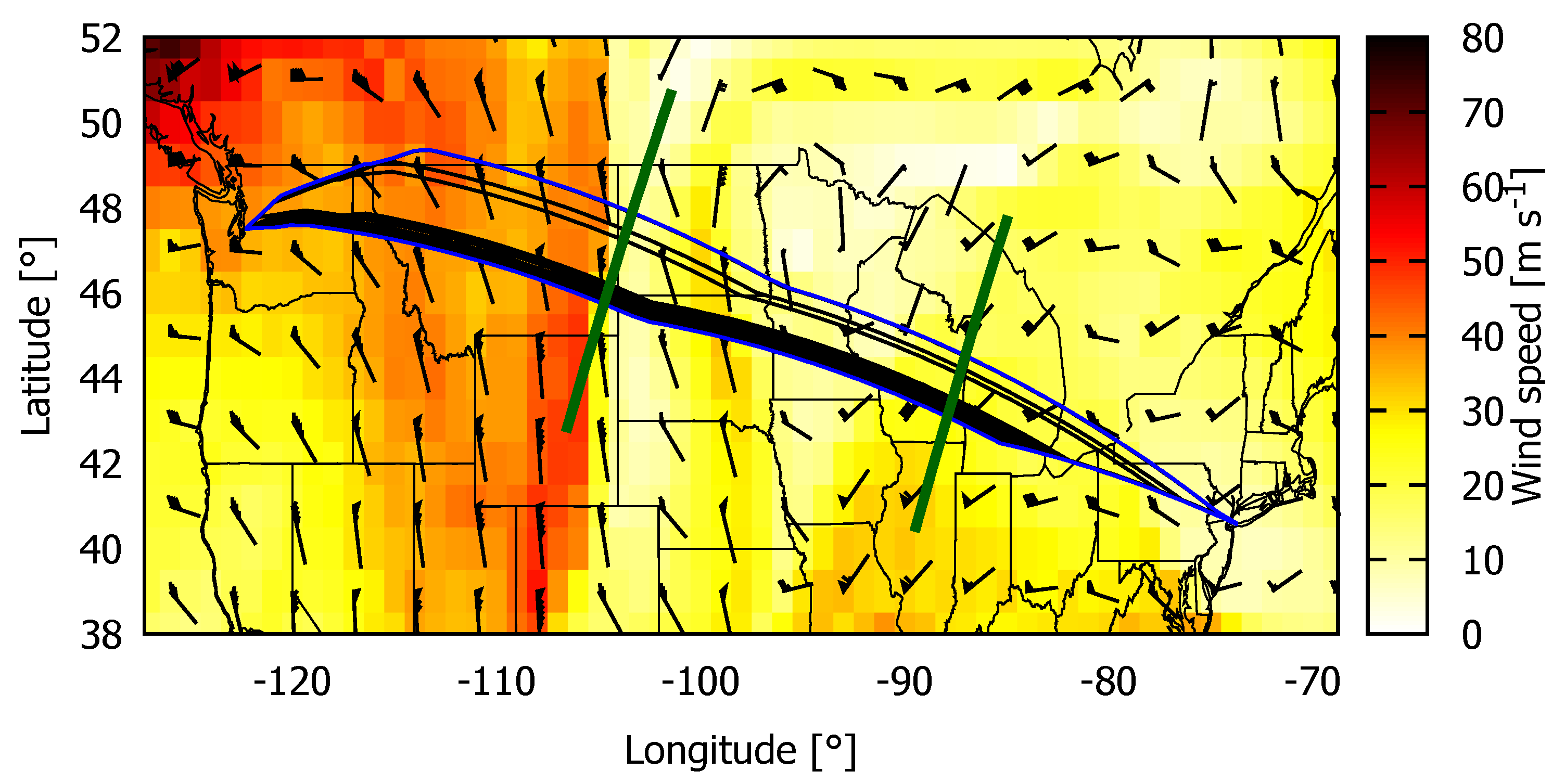
Figure 9 depicts the CoO described by a set of 380 geographic coordinates for a sample flight on 31 January 2020. The GEFS-optimized flight paths have an average ground distance of 3920 km ( = km) and an average air distance of 3519 km ( = km). The minimum cruising altitude is 206 hPa (≈380 FL), and the maximum is 194 hPa (≈390 FL). To avoid altitude-dependent fluctuations in the fuel consumption, the altitude is fixed at the average value for the subsequent fuel-saving potential computations. The CoO has a maximum width of LW = 259 km, which can be reduced significantly to LW = 71 km by removing the three northernmost flights.
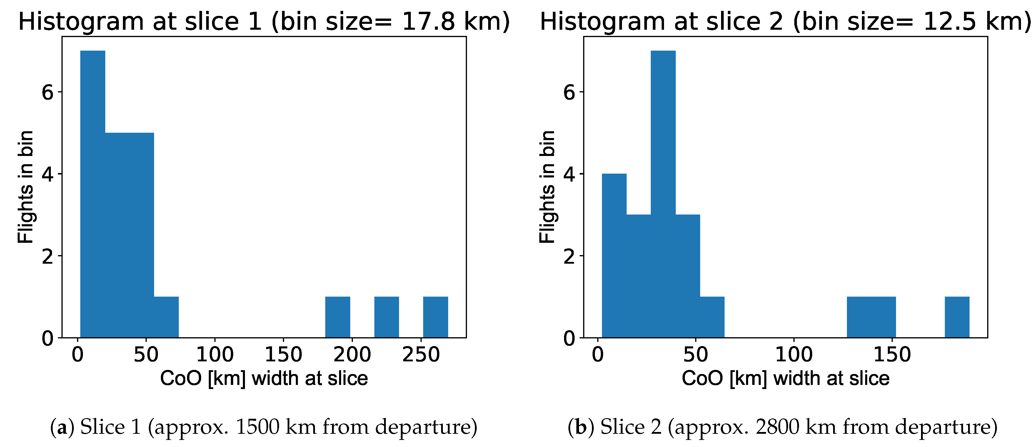
This reduction potential is shown by the two slices indicated as green lines in Figure 9. Figure 10 contains histograms for the two slices, which show the distribution of ensemble flights over the width of the corridor (starting at the southern border of the CoO). As mentioned above, a reduction of width can be achieved by eliminating the ensemble flights on the far right of the histograms. Furthermore, the location of the actual route can be described probabilistically. In the case of Figure 9, it is most likely that the route of the actual flight is near the southern border. This parameter may help to manage ATFM capacity planning. The minimum width of the CoO is close to the airports with LW = km. With an average width of LW = 161 km, the entire CoO is much larger than the 2 × 37 km of the RNP20 requirements [2] used for ATS route spacing. However, the reduced CoO fulfills these requirements with its maximum width and is even close to the containment area of the RNP10 (4 × 18.3 km). The LWSD of the complete CoO is km and the PP score is . With a total area of km2, the corridor requires an AR = km2 km.
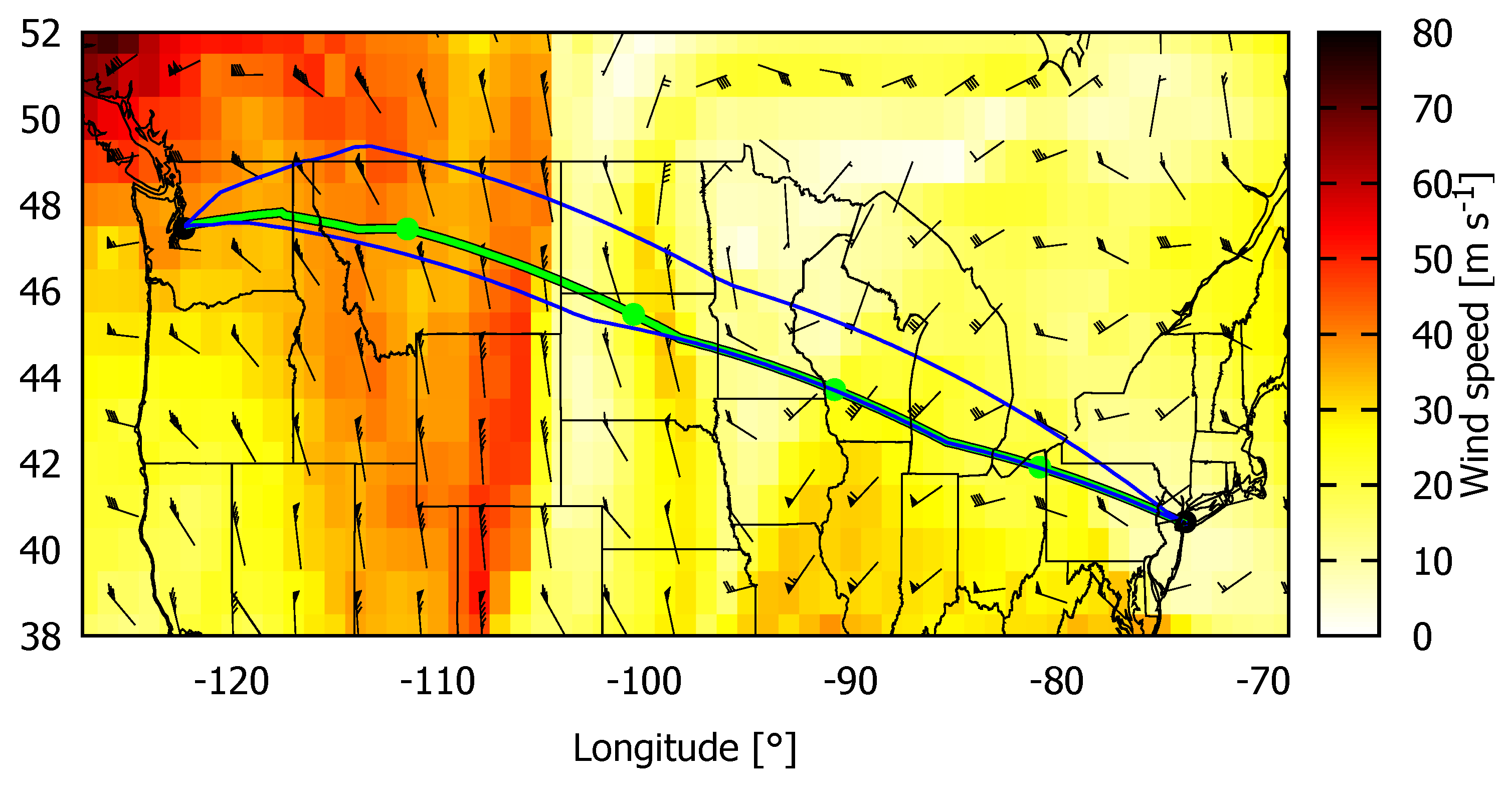
Figure 11 shows hourly re-optimized flights as lines and the re-optimization coordinates as dots, respectively. The green line indicates the flight, which is restricted to the shape of the CoO. As a reference, a freely optimized flight without CoO restriction is included in black. It turns out that the chosen corridor is sufficiently dimensioned because the unrestricted flight equals the CoO-constrained flight. Assuming the latest RAP cycle represents the real atmosphere, the hourly in-flight optimization saves 139 kg fuel compared to the trajectory filed pre-departure, which has been optimized in GFS weather (nominal 9322 kg fuel burn).
4.2. Aggregated Results for August 2019 and January 2020
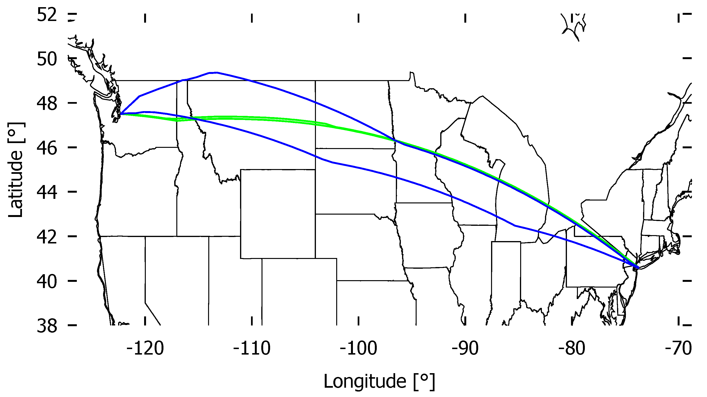
In the following section, the results from Section 4.1 are presented for August 2019 and January 2020. Figure 12 shows the minimum (29th) and maximum (31st) area of the calculated CoO in January 2020. A clear variance in CoO size can be seen, although these two days are close in time. The other calculated CoO for this month are mainly located within the blue hull, but shifted to the north or south, depending on the high-level winds at each day.
Table 3 lists LW, AR, PP aggregated for each month. This analysis highlights that the difference between a winter or a summer month has only a minor influence on the shape of the CoO. In general, the CoOs tend to cover a larger area in the summer month, since the weather variability is also higher (cf. Section 2.1). However, there are fewer differences in the maximum extent of the CoO. The high values in the maximum area coverage are mainly driven by some single flights, which seem to cover an extreme scenario. Removing these outliers would bring the maximum value significantly closer to the mean value.
Table 3 also shows results for the in-flight optimization, on the one hand considering the CoO hull and on the other hand without this limitation. Basically, an average saving of 66 kg ( %) fuel is shown, if hourly weather updates are used to optimize the remaining flight route within the CoO. However, an average saving of 80 kg fuel could be achieved if the corridor boundaries were not used and the optimization process could be more flexible. The calculated Polsby–Propper score (PP) is very small, which means that the resulting CoO is far from being a circle. The differences in cruising altitude between the ensemble optimized flights are marginal, the height of the CoO is typically between 0 and 400 m. This is often within the limits of the Reduced Vertical Separation Minima (RVSM).
Figure 13 shows the average area AR needed for each month as a box plot, where Figure 14 gives more details in LW for all CoO from January 2020. To summarize, there is a tendency for the unrestricted in-flight optimization to leave the CoO with large lateral dimension more often (due to the greater weather variability).
5. Conclusions and Outlook
In this study, the concept of establishing so-called CoOs encasing flight trajectories was introduced. A CoO is designed based on GEFS weather ensemble forecasts to consider the uncertain environmental conditions before and during flight. Within the CoO, the flight plan was allowed to be freely adopted (re-optimized) based on hourly updated weather cycles (RAP), provided for use cases in the U.S. airspace. By limiting the CoO to certain boundaries, the solution space for re-optimization was limited to support the predictability for ATM.
The case study was applied to two non-consecutive months of weather data. It has been proven that optimization during flight offers potential for fuel savings, even inside the CoO boundaries based on known uncertainties in the weather before departure. A tendency for higher variability of the weather parameter, observed in the summer month August 2019, can be directly transferred to a tendency for a larger required area of the CoO. The vertical extent of the corridor representing flight altitudes shows only little variation within the scenarios. Although some CoOs were deemed too small, the majority of the possible savings were still achieved within the CoO restrictions. To reduce the probability to leave the CoO, its borders should be extended by an increased variation of the weather parameters or an additional constant margin, so that, e.g., with a significance level of 95%, all flights are included. Statistical methods, e.g., the fitting of the weather uncertainties to a distribution function, may also be used to increase the robustness of the CoO generation. However, this might introduce additional modeling errors, which increase the uncertainty and the CoO size unexpectedly as a consequence.
For ATM planning stability, here separated from capacity, a reduction of the CoO width, at least regionally, is the more interesting choice. When slicing along the corridor (see Figure 9), outliers can be found and eliminated to provide the most effective approach to reduction, while still considering the most probable routing area of the aircraft. This way, the airspace capacity might be increased by removing trajectories from the CoO set or by restricting parts of the CoO to existing ATS routes in very dense airspaces. Another approach would be to narrow the CoO to the first calculated segment at the outbound side to ensure simpler planning, especially in the departure area. However, since there can be a considerable amount of time between calculating the CoO in the flight-planning phase and the flight itself, overly narrowing of the CoO contradicts the general approach and will not be pursued further at the moment.
To summarize, providing a CoO is useful in terms of achieving further trajectory optimization potential. Thus far, the CoO design assumes a single flight perspective only. In order to implement this concept in the airspace, further investigations regarding interdependencies between other airspace users and their CoO and thus the impact to airspace capacity should be carried out.
The CoO provides a trade-off between an increased fuel-saving potential with more flexibility in-flight optimization and a certain degree of airspace capacity planning reliability. Therefore, the CoO enables the transition of today’s airspace to completely free optimization airspace. To conclude, the applicability of CoO in ATM still needs to be examined. In a further step, the capacity will be quantified in an ATM traffic scenario, e.g., by analyzing the total required area per ATC sector. However, we assume that the actual impact on the operational workload of the controller to monitor traffic and avoid conflicts will remain low due to similar aircraft headings as well as entry and exit times. The same applies to the change in sector capacity based on this workload.
A further challenge is how to deal with determining the size of the CoO from the operational point of view. Airlines will tend to choose the largest possible space for a maximum of flexibility, which increases the risk for capacity bottlenecks. In this paper, the CoO was designed to the minimum reasonable size from the optimization perspective. The ATM agencies might enforce this restriction. Another option is the introduction of financial incentives, e.g., a charge relative to the filed CoO width. This approach, however, is highly sensitive because it might diminish the desired fuel-saving potential. In general, measures to counter excessive use of the CoO must be discussed concerning ATC capacity, which is of interest for further research.
Author Contributions
M.L. devised the project, the main conceptual ideas, and proof outline. M.L., J.R., and T.Z. worked out almost all of the technical details, and performed the numerical calculations for the experiment. M.L. designed the model and the computational framework and analyzed the data. J.R. worked out the uncertainty of weather forecasts. M.L., J.R., T.Z., and H.F. wrote the manuscript. H.F. helped with supervising the project. All authors have read and agreed to the published version of the manuscript.
Funding
This work has been done in the framework of the project “Improved planning and realization of flight profiles with the lowest ecological footprint and minimum fuel consumption (ProfiFuel)”, financed by the Federal Ministry for Economic Affairs and Energy (BMWI), and the project “Enhanced Flight Planning by introducing stochastic trajectory data (UTOPIA II)”, financed by Deutsche Forschungsgemeinschaft e.V. (DFG).
Conflicts of Interest
The authors declare no conflict of interest.
Abbreviations
The following abbreviations are used in this manuscript:
| ACARS | Aircraft Communications Addressing and Reporting System |
| AIRAC | Aeronautical Information Regulation and Control |
| AMDAR | Aircraft Meteorological Data Relay |
| ASDAR | Aircraft to Satellite Data Relay |
| ATC | Air Traffic Control |
| ATFM | Air Traffic Flow Management |
| ATM | Air Traffic Management |
| BADA | Base of Aircraft Data |
| COALA | COmpromized Aircraft performance model with Limited Accuracy |
| CoO | Corridor of Optimization |
| ECMWF | European Center for Medium-Range Weather Forecasts |
| EFB | Electronic Flight Bag |
| GDAS | Global Data Assimilation System |
| GEFS | Global Ensemble Forecast System |
| GFS | Global Forecast System |
| NCEP | National Centers for Environmental Prediction |
| NCEP | National Centers for Environmental Prediction |
| NOAA | National Oceanic and Atmospheric Administration |
| NWS | National Weather Service |
| PBN | Performance Based Navigation |
| RAP | Rapid Refresh |
| RNAV | Area Navigation |
| RNP | Required Navigation Performance |
| TOC | Top of Climb |
| TOD | Top of Descent |
| TOMATO | TOolchain for Multi-criteria Aircraft Trajectory Optimization |
| VHF | Very High Frequency |
References
- “PANS-ATM, Procedures for Navigation Services—Air Traffic Management” Doc 4444, 16th ed.; International Civil Aviation Organization: Montreal, QC, Canada, 2016.
- Performance-Based Navigation (PBN) Manual; International Civil Aviation Organization: Montreal, QC, Canada, 2013.
- Rosenow, J.; Strunck, D.; Fricke, H. Trajectory optimization in daily operations. CEAS Aeronaut. J. 2019. [Google Scholar] [CrossRef]
- Pabst, T.; Kunze, T.; Schultz, M.; Fricke, H. Modeling External Disturbances for Aircraft in Flight to Build Reliable 4D Trajectories. In Proceedings of the International Conference on Application and Theory of Automation in Command and Control Systems (ATACCS), Naples, Italy, 28–30 May 2013; pp. 3519–3523. [Google Scholar]
- Lindner, M.; Rosenow, J.; Fricke, H. Aircraft trajectory optimization with dynamic input variables. CEAS Aeronaut. J. 2019. [Google Scholar] [CrossRef]
- Evans, A.D.; Lee, P.U. Using Machine-Learning to Dynamically Generate Operationally Acceptable Strategic Reroute Options. In Proceedings of the Thirteenth USA/Europe Air Traffic Management Research and Development Seminar (ATM2019), Vienna, Austria, 17–21 June 2019. [Google Scholar]
- Li, X.; Nair, P.; Zhang, Z.; Gao, L.; Gao, C. Aircraft Robust Trajectory Optimization Using Nonintrusive Polynomial Chaos. J. Aircr. 2014, 51, 1592–1603. [Google Scholar] [CrossRef]
- González-Arribas, D.; Soler, M.; Sanjurjo-Rivo, M.; García-Heras, J.; Sacher, D.; Gelhardt, U.; Lang, J.; Hauf, T.; Simarro, J. Robust Optimal Trajectory Planning Under Uncertain Winds and Convective Risk. In Air Traffic Management and Systems III; Institute, E.N.R., Ed.; Springer: Singapore, 2019; pp. 82–103. [Google Scholar]
- García-Heras Carretero, J.; Soler, M.; González Arribas, D. Characterization and Enhancement of Flight Planning Predictability under Wind Uncertainty. Int. J. Aerosp. Eng. 2019, 2019, 1–29. [Google Scholar] [CrossRef]
- Legrand, K.; Puechmorel, S.; Delahaye, D.; Zhu, Y. Aircraft trajectory planning under wind uncertainties. In Proceedings of the 2016 IEEE/AIAA 35th Digital Avionics Systems Conference (DASC), Sacramento, CA, USA, 25–29 September 2016; pp. 1–9. [Google Scholar]
- Franco, A.; Rivas, D.; Valenzuela, A. Optimal Aircraft Path Planning in a Structured Airspace Using Ensemble Weather Forecasts. Sesar Innov. Days 2018, 2018, 1–7. [Google Scholar]
- Rivas, D.; Franco, A.; Valenzuela, A. Analysis of aircraft trajectory uncertainty using Ensemble Weather Forecasts. In Proceedings of the 7th European Conference for Aeronautics and Space Sciences (EUCASS), Milano, Italy, 4–9 July 2017. [Google Scholar]
- Cheung, J.; Hally, A.; Heijstek, J.; Marsman, A.; Brenguier, J.L. Recommendations on trajectory selection in flight planning based on weather uncertainty. Sesar Innov. Days 2015, 2015, 1–8. [Google Scholar]
- Lindner, M.; Zeh, T.; Fricke, H. Reoptimization of 4D-flight trajectories during flight considering forecast uncertainties. In Proceedings of the Deutscher Luft- und Raumfahrtkongress, Friedrichshafen, Germany, 4–6 September 2018. [Google Scholar]
- Rosenow, J.; Förster, S.; Lindner, M.; Fricke, H. Multicriteria-Optimized Trajectories Impacting Today’s Air Traffic Density, Efficiency, and Environmental Compatibility. J. Air Transp. 2019, 27, 8–15. [Google Scholar] [CrossRef]
- Förster, S.; Rosenow, J.; Lindner, M.; Fricke, H. Toolchain for Optimizing Trajectories under real Weather Conditions and Realistic Flight Performance. In Proceedings of the Greener Aviatian, Brussels, Belgium, 11–13 October 2016. [Google Scholar]
- Wing, D.; Burke, K.; Ballard, K.; Henderson, J.; Woodward, J. Initial TASAR Operations Onboard Alaska Airlines. In Proceedings of the AIAA Aviation 2019 Forum, Dallas, TX, USA, 17–21 June 2019. [Google Scholar]
- World Meteorological Organization. Aircraft Meteorological Data Relay (AMDAR) Reference Manual; World Meteorological Organization: Geneva, Switzerland, 2003. [Google Scholar]
- NOAA NCEP Global Ensemble Forecast System (GEFS). Available online: https://www.emc.ncep.noaa.gov/users/verification/global/gefs/ops/ (accessed on 2 July 2020).
- Ballish, B.A.; Kumar, V.K. Systematic Differences in Aircraft and Radiosonde Temperatures. Bull. Am. Meteorol. Soc. 2008, 89, 1689–1708. [Google Scholar] [CrossRef]
- Brodsky, I. H3, a hierarchical hexagonal geospatial indexing system. Uber Open Source. 2019. Available online: https://uber.github.io/h3/ (accessed on 2 July 2020).
- Rosenow, J.; Fricke, H. Flight Performance Modeling to optimize Trajectories. In Proceedings of the Deutscher Luft- und Raumfahrtkongress, Braunschweig, Germany, 13–15 September 2016. [Google Scholar]
- Rosenow, J.; Förster, S.; Fricke, H. Continuous Climb Operations with Minimum Fuel Burn. In Proceedings of the Sixth SESAR Innovation Days, Delft, The Netherlands, 8–10 November 2016. [Google Scholar]
- Bellock, K.E. Python Alphashape Library, v1.0.1. Available online: https://alphashape.readthedocs.io (accessed on 2 July 2020).
- Polsby, D.D.; Popper, R.D. The Third Criterion: Compactness as a Procedural Safeguard Against Partisan Gerrymandering. Yale Law Policy Rev. 1991, 9, 301–353. [Google Scholar] [CrossRef]
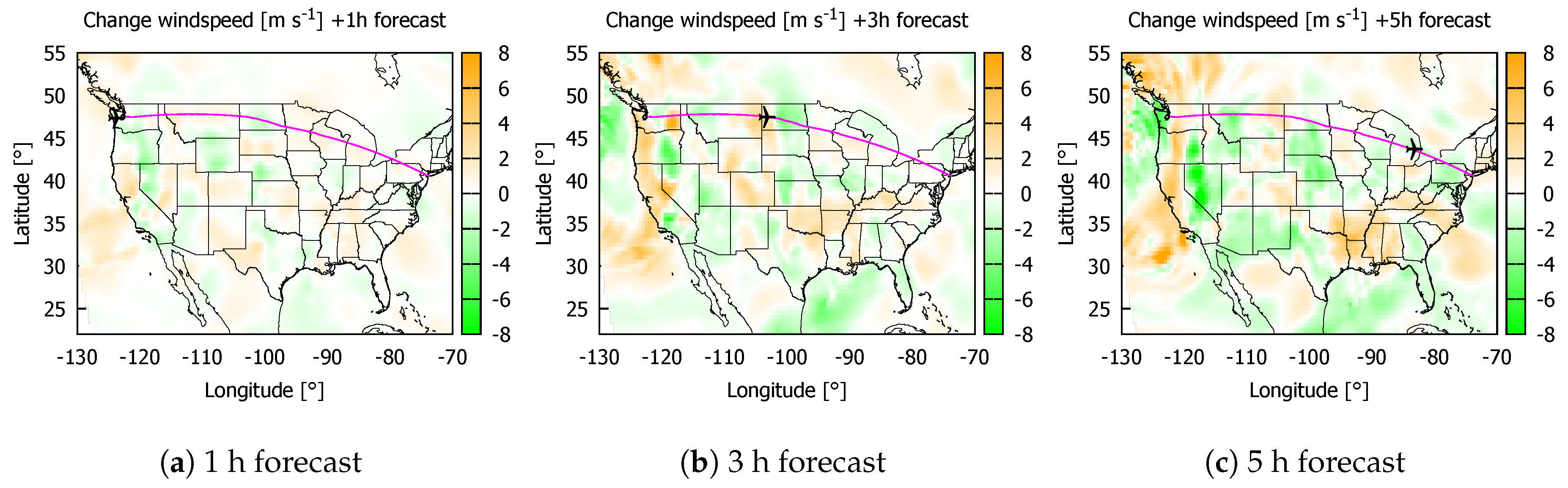
Figure 1.
Increasing inaccuracy of weather forecasts shown as differences in wind speed [m s] between the used weather cycle (GFS, 31 January 2020, Cycle 00) before departure (a), and the latest available Rapid Refresh cycle during flight (b,c). More intensive colors mean more erroneous forecasts.
Figure 1.
Increasing inaccuracy of weather forecasts shown as differences in wind speed [m s] between the used weather cycle (GFS, 31 January 2020, Cycle 00) before departure (a), and the latest available Rapid Refresh cycle during flight (b,c). More intensive colors mean more erroneous forecasts.

Figure 2.
Mean differences in wind speed for 29th (a) and 31st (b) January 2020 between a six-hour GFS forecast and the corresponding GFS model output (six hours after the forecast has been calculated). On a global average, the GFS modeled mean wind speed deviates 3 m s from the AMDAR output of the same time.

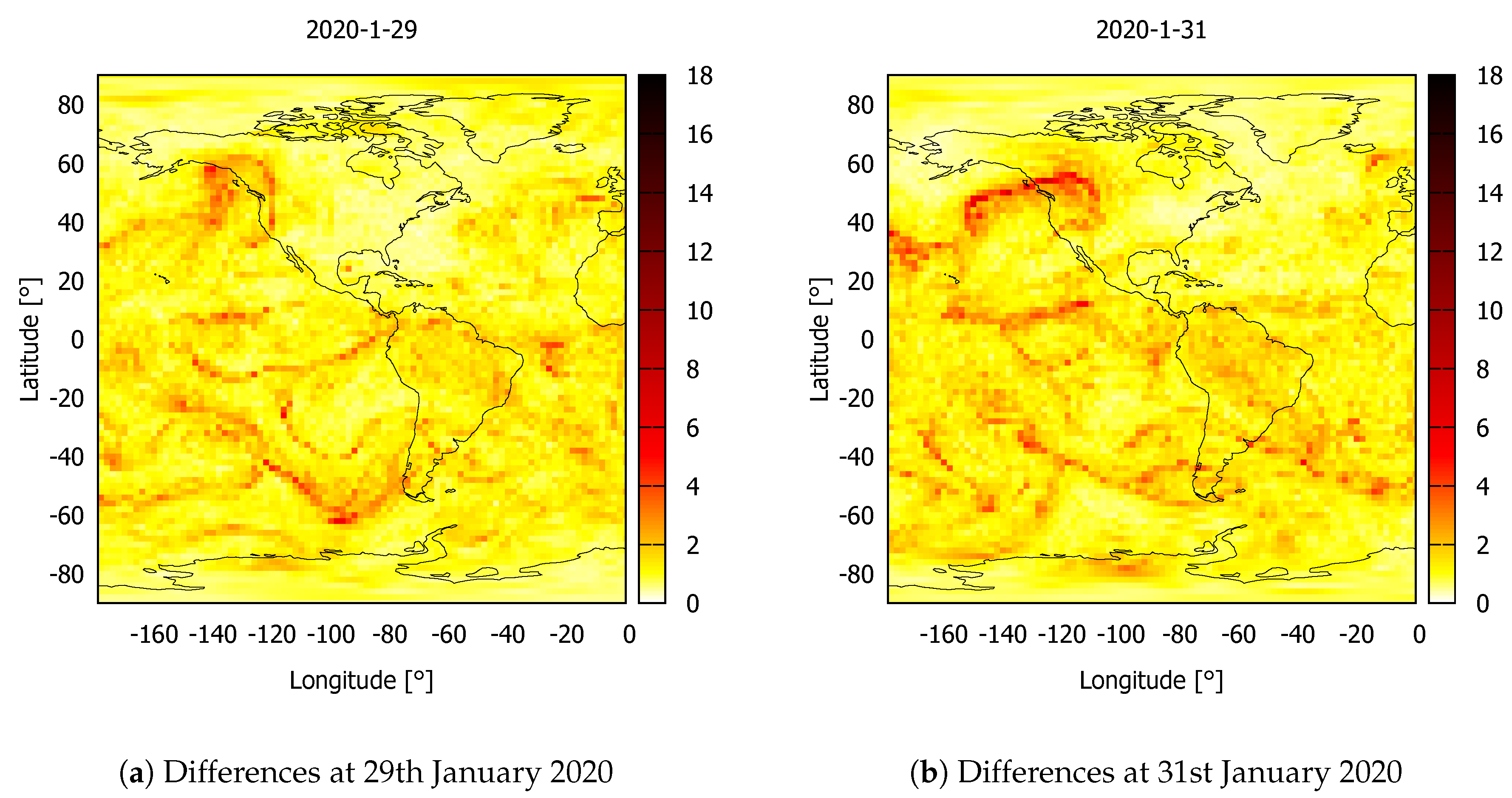
Figure 3.
Monthly mean differences between the mean of 21 six-hour GEFS ensemble forecasts (calculated at 12:00 p.m./cycle 00) and the corresponding GFS model output at 6:00 a.m. in January 2020 (cycle 06). On a global average, the ensemble mean wind speed deviates m s from the GFS model output of the same time. Maximum differences of m s have been detected in this month.

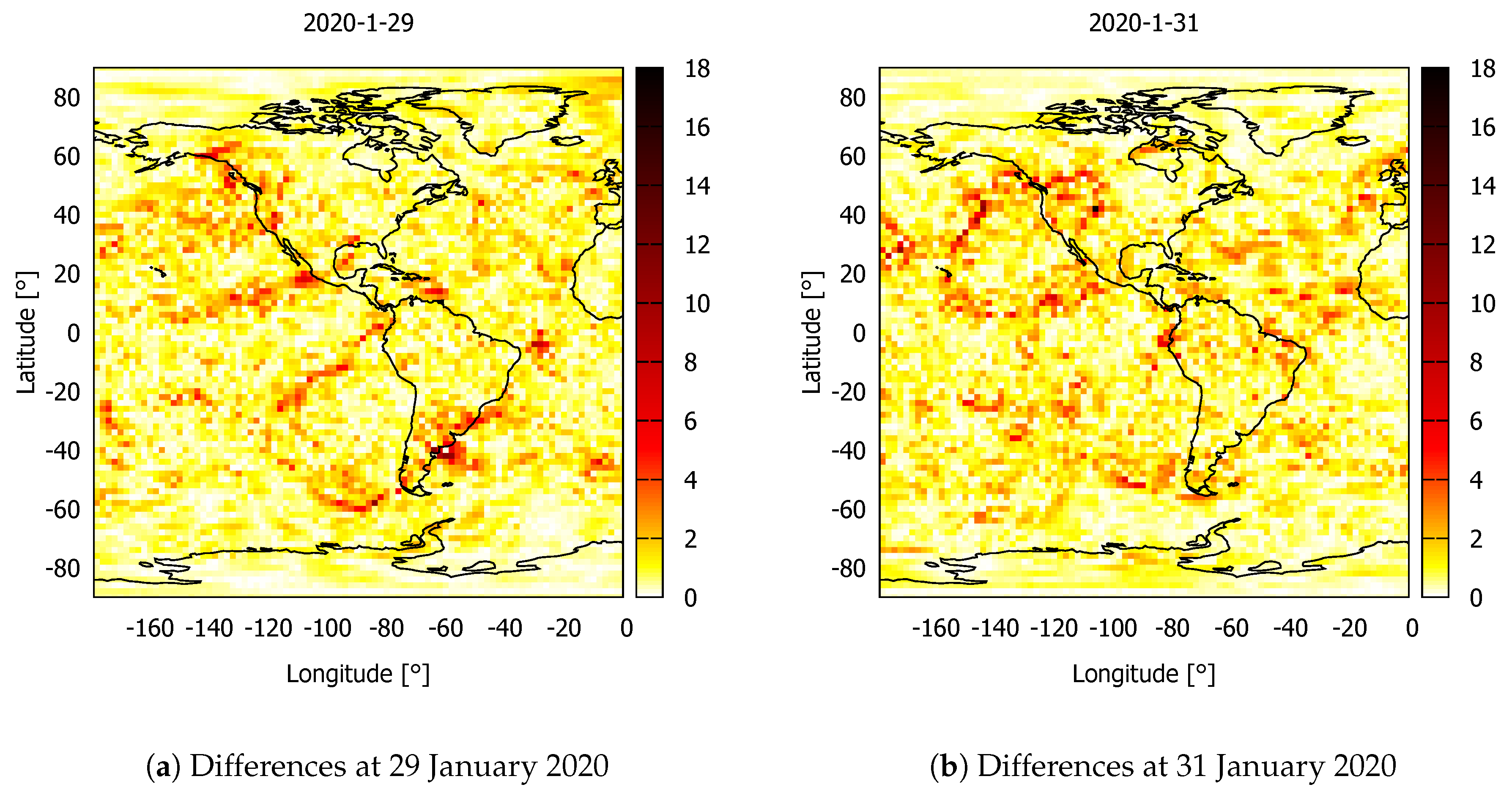
Figure 4.
Standard deviation of 21 six-hour GEFS forecasts for the 29th (a) and 31st (b) January 2020. On a global average, the ensemble mean wind speed scatters 6 m s around the mean.
Figure 4.
Standard deviation of 21 six-hour GEFS forecasts for the 29th (a) and 31st (b) January 2020. On a global average, the ensemble mean wind speed scatters 6 m s around the mean.

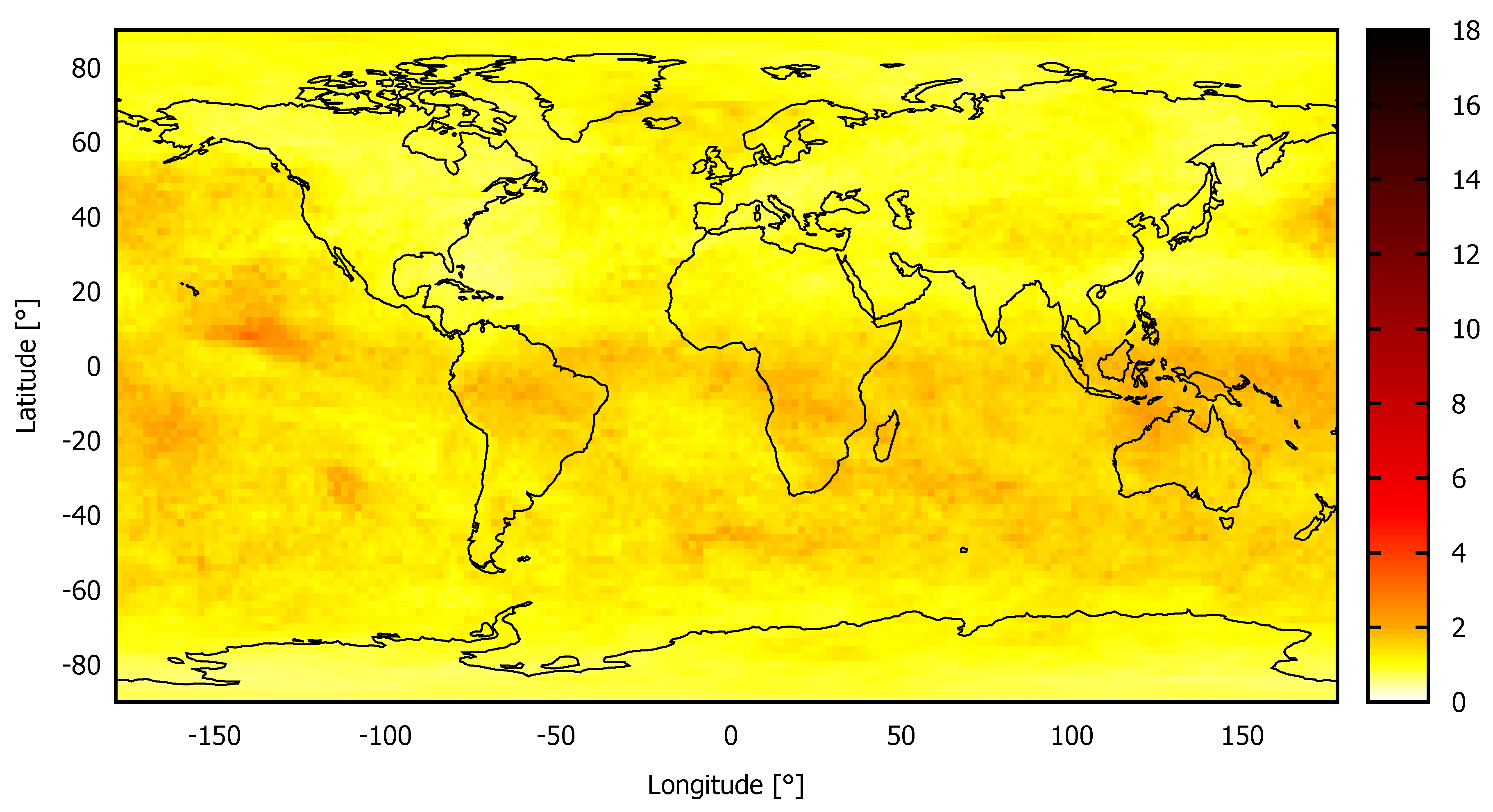
Figure 5.
Mean differences in local wind speed between aircraft measured AMDAR data and the closest global GFS model output on 29 January 2020. On average, the GFS modeled mean wind speed deviates 3 m s from the AMDAR output at the same time. Additionally, the global distribution of AMDAR measurements can be detected.

Figure 6.
Hexagonal path search with neighbor ring (left) and neighbor rings (right).

Figure 7.
2D CoO generation from three ensemble trajectories (left) to a concave shape encasing all waypoints (right).
Figure 7.
2D CoO generation from three ensemble trajectories (left) to a concave shape encasing all waypoints (right).

Figure 8.
CoO solution space (grey) with two re-optimizations of the trajectory during flight (Reopt 1, Reopt 2). Different line types represent the best flight path after each re-optimization. The blue line shows the additional buffer enveloping the CoO.
Figure 8.
CoO solution space (grey) with two re-optimizations of the trajectory during flight (Reopt 1, Reopt 2). Different line types represent the best flight path after each re-optimization. The blue line shows the additional buffer enveloping the CoO.

Figure 9.
The set of 21 ensemble trajectories (black) for each ensemble forecast of 31 January 2020, Cycle 00, and the resulting CoO (blue). The heat map indicates wind speed with arrows for the wind direction (0–40 m s) at the cruising altitude of approx. FL 370.
Figure 9.
The set of 21 ensemble trajectories (black) for each ensemble forecast of 31 January 2020, Cycle 00, and the resulting CoO (blue). The heat map indicates wind speed with arrows for the wind direction (0–40 m s) at the cruising altitude of approx. FL 370.

Figure 10.
Histogram of the lateral distribution of flights in the CoO for two slices (dark green lines in Figure 9). The measurement of the width starts at the southern border of the CoO.
Figure 10.
Histogram of the lateral distribution of flights in the CoO for two slices (dark green lines in Figure 9). The measurement of the width starts at the southern border of the CoO.

Figure 11.
In-flight re-optimized trajectories on 31st January 2020, where the green trajectory is restricted to the CoO hull, while the black trajectory is freely optimized. In-flight re-optimizations are calculated at 1:00 a.m., 2:00 a.m., 3:00 a.m., and 4:00 a.m. UTC.
Figure 11.
In-flight re-optimized trajectories on 31st January 2020, where the green trajectory is restricted to the CoO hull, while the black trajectory is freely optimized. In-flight re-optimizations are calculated at 1:00 a.m., 2:00 a.m., 3:00 a.m., and 4:00 a.m. UTC.

Figure 12.
Plot of the smallest (29th, green) and largest (31st, blue) CoO by area in January 2020 for the flight KSEA-KJFK, 12:00 a.m. UTC departure time.
Figure 12.
Plot of the smallest (29th, green) and largest (31st, blue) CoO by area in January 2020 for the flight KSEA-KJFK, 12:00 a.m. UTC departure time.

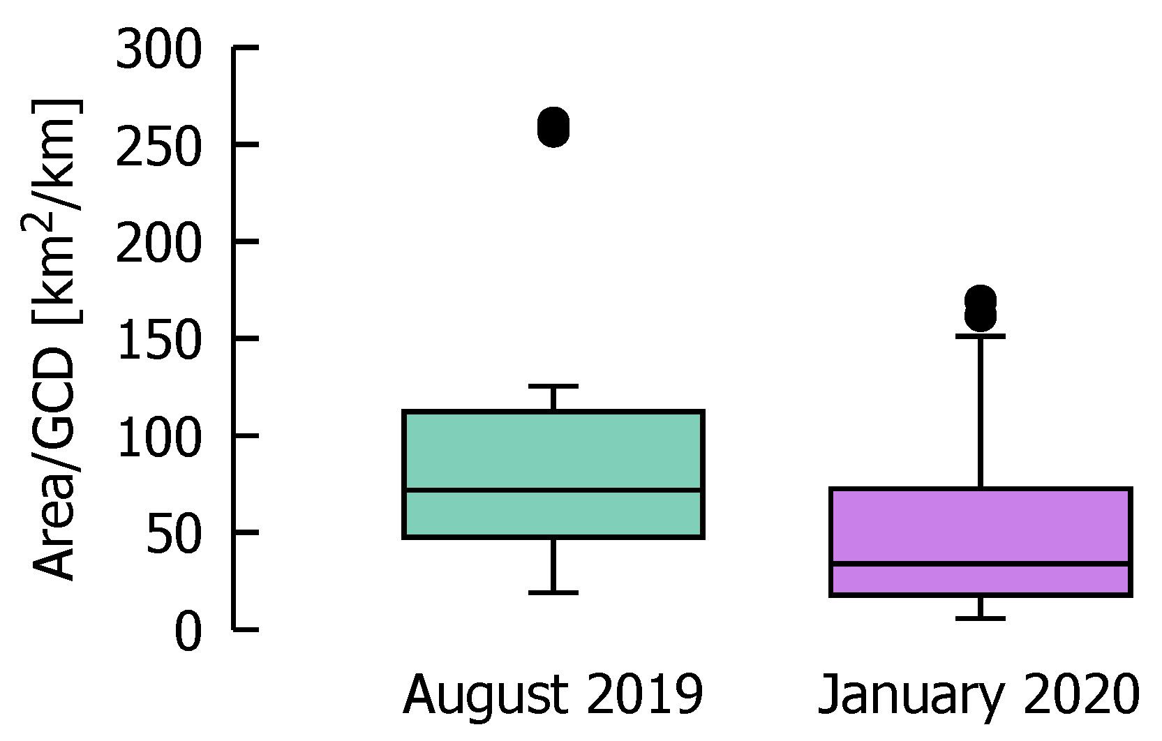
Figure 13.
Comparison of CoO area per km great circle distance (km2 km−1) for August 2019 and January 2020. The outliers shown here result from significantly increased CoO, often caused by one ensemble trajectory. Ignoring this for the sake of remaining air space capacity would reduce the area.
Figure 13.
Comparison of CoO area per km great circle distance (km2 km−1) for August 2019 and January 2020. The outliers shown here result from significantly increased CoO, often caused by one ensemble trajectory. Ignoring this for the sake of remaining air space capacity would reduce the area.

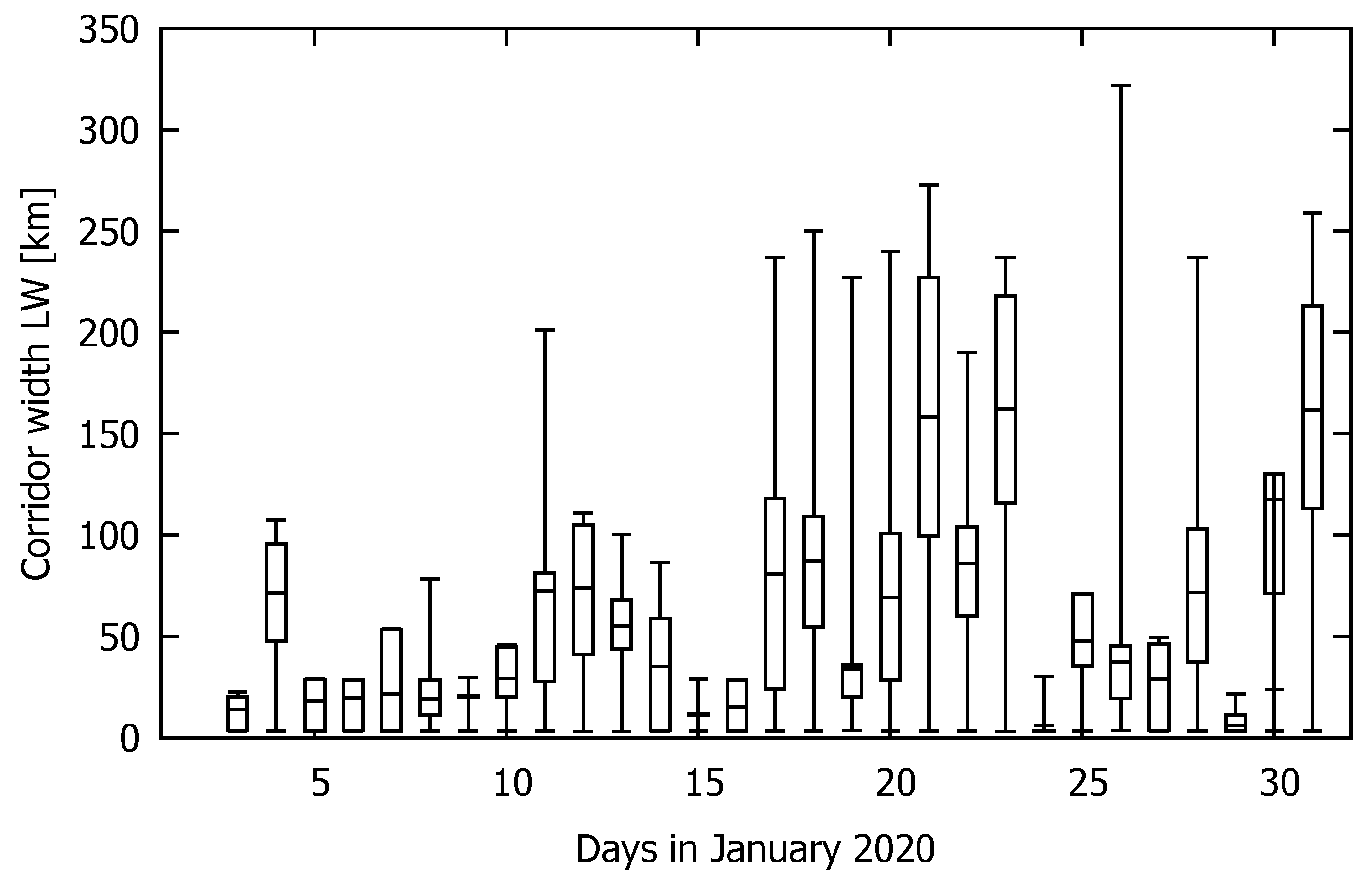
Figure 14.
Box plot of CoO width LW (km) of each day in January 2020.


Table 1.
Scenario input parameters.
| Departure | KSEA (Seattle) |
| Destination | KJFK (New York) |
| Great circle distance | 4480 km |
| Aircraft | A320-212, CFM-56 engine |
| Payload | 10,000 kg |
| Take off fuel | 11,000 kg |
| Take off time | 00:00 UTC |
| Date | August 2019, January 2020 |
Table 2.
Weather input parameters.
| GFS | GEFS | RAP | |
|---|---|---|---|
| Pressure altitudes [hPa] | 150, 175, [200 … 900, 50], 925, 1000 | 150, 200, 250, 350, [450 … 900, 50], 925, 1000 | [150 … 1000, 25] |
| Spatial resolution | 0.5, C00 | 0.5, C00 | 0.25, |
| Temporal resolution | 4 cycles/day, forecast 3, 6 h | 4 cycles/day, forecast 6 h | hourly cycles and forecasts |
| Parameters | Wind U (UGRD), V (VGRD), Temperature (TMP), Relative humidity (RH), Geopotential height (HGT), and Pressure altitude (PRES) | ||
Table 3.
CoO characteristics for August 2019 and January 2020.
| August 2019 | January 2020 | ||
|---|---|---|---|
| Width LW [km] | Avg | 68 | 56.1 |
| SD | 45.4 | 46.7 | |
| Max | 257.8 | 214.6 | |
| Area/GCD AR [km2 km] | Avg | 66.9 | 53.24 |
| SD | 30.3 | 44.8 | |
| Max | 145.5 | 169 | |
| Polsby Propper Score PP | Avg | 0.05 | 0.04 |
| SD | 0.02 | 0.03 | |
| Max | 0.098 | 0.13 | |
| Height H [m] | Avg | 138 | 70 |
| Min | 0 | 0 | |
| Max | 560 | 380 | |
| Number of flights left the CoO during in-flight optimization | 13 of 24 | 14 of 29 | |
| Avg fuel saving [kg] in-flight opt within CoO | 67 | 65 | |
| Avg fuel saving [kg] in-flight opt without CoO | 80 | 81 | |
© 2020 by the authors. Licensee MDPI, Basel, Switzerland. This article is an open access article distributed under the terms and conditions of the Creative Commons Attribution (CC BY) license (http://creativecommons.org/licenses/by/4.0/).
Share and Cite
MDPI and ACS Style
Lindner, M.; Rosenow, J.; Zeh, T.; Fricke, H. In-Flight Aircraft Trajectory Optimization within Corridors Defined by Ensemble Weather Forecasts. Aerospace 2020, 7, 144. https://doi.org/10.3390/aerospace7100144
AMA Style
Lindner M, Rosenow J, Zeh T, Fricke H. In-Flight Aircraft Trajectory Optimization within Corridors Defined by Ensemble Weather Forecasts. Aerospace. 2020; 7(10):144. https://doi.org/10.3390/aerospace7100144
Chicago/Turabian StyleLindner, Martin, Judith Rosenow, Thomas Zeh, and Hartmut Fricke. 2020. "In-Flight Aircraft Trajectory Optimization within Corridors Defined by Ensemble Weather Forecasts" Aerospace 7, no. 10: 144. https://doi.org/10.3390/aerospace7100144
Note that from the first issue of 2016, this journal uses article numbers instead of page numbers. See further details here.