Evaluation of Time Difference of Arrival (TDOA) Networks Performance for Launcher Vehicles and Spacecraft Tracking


1
Department of Mechanical and Aerospace Engineering (DIMA), Sapienza University of Rome, via Eudossiana 18, 00184 Rome, Italy
2
Department of Astronautics, Electric and Energy Engineering (DIAEE), Sapienza University of Rome, via Eudossiana 18, 00184 Rome, Italy
*
Author to whom correspondence should be addressed.
Aerospace 2020, 7(10), 151; https://doi.org/10.3390/aerospace7100151
Submission received: 31 August 2020
/
Revised: 14 October 2020
/
Accepted: 16 October 2020
/
Published: 20 October 2020
(This article belongs to the Special Issue Orbit Determination of Earth Orbiting Objects)
Abstract
:Time Difference of Arrival (TDOA) networks could support spacecraft orbit determination or near-space (launcher and suborbital) vehicle tracking for an increased number of satellite launches and space missions in the near future. The evaluation of the geometry of TDOA networks could involve the dilution of precision (DOP), but this parameter is related to a single position of the target, while the positioning accuracy of the network with targets in the whole celestial vault should be evaluated. The paper presents the derivation of the MDOP (minimum dilution of precision), a parameter that can be used for evaluating the performance of TDOA networks for spacecraft tracking and orbit determination. The MDOP trend with respect to distance, number of stations and target altitude is reported in the paper, as well as examples of applications for network performance evaluation or time precision requirement definitions. The results show how an increase in the baseline enables the inclusion of more impactive improvements on the MDOP and the mean error than an increase in the number of stations. The target altitude is demonstrated as noninfluential for the MDOP trend, making the networks uniformly applicable to lower altitude (launchers and suborbital vehicles) and higher altitude (Low and Medium Earth Orbits satellites) spacecraft.
Keywords:
Time Difference of Arrival; satellite; launchers; suborbital; orbit determination; tracking; hyperbolic; TDOA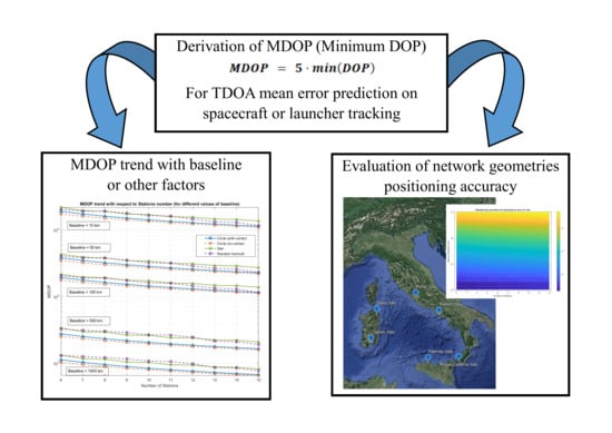
1. Introduction
The significant increase in satellite launches, alongside the rise of new mission concepts for small satellite megaconstellations [1], launcher vehicles and even commercial suborbital transportation [2] systems are requiring an increase in tracking and orbit determination system capacity. The improvements to be introduced have the dual objective of maintaining a position and orbit determination accuracy suitable for the operations of all the users and of ensuring the sustainability of the environment by efficiently managing space traffic [3].
If, nowadays, satellite tracking data acquisition is mainly performed by active surveillance systems, i.e., primary radars and laser ranging, often supported by optical observations [4], the implementation of multilateration systems offers interesting perspectives for spacecraft tracking and orbit determination [5,6]. In particular, these systems are able to achieve position determination when deploying a network of distributed sensors. Multilateration methods are based on the retrieval of the motion state of a target without processing any information sent by the target itself. The dependability is thus constrained by the effective presence and well-functioning of a transmitting system on-board the target, but not, for example, by the accuracy, correctness or truthfulness of the spaceborne sensor data, which are not considered for determining the position. One of the most implemented multilateration algorithms is the Time Difference of Arrival (TDOA [7]), aimed at reconstructing the target location by analyzing the differences between the reception times of signals emitted by the target. The target position is calculated by evaluating the intersection of the hyperboloids that mark a constant difference in time of arrival between each pair of stations. The method is often used for terminal aircraft tracking [8,9,10], indoor positioning [11,12,13,14] and other applications. TDOA could be easily applicable for supporting orbit determination and spacecraft tracking, as all the operational potential targets down-link frequencies (e.g., of the beacon or telemetry channels) are well-known and often concentrated in a limited number of bands [15,16,17]. This method could also be supporting near-space flights, such as launcher missions, stratospheric balloons [18] and suborbital flights [2]. The nature of the targets, i.e., high altitude vehicles, allows for a wide accessibility of their signals from the ground, thus improving the impact of a wide baseline network for TDOA positioning and orbit determination. The set-up of similar networks could be eased by the implementation of low-cost, flexible radio systems such as software defined radios (SDRs), able to operate in an extended frequency range and to manage a multiplicity of the needed tasks for acquiring the measurements and to intersect them in order to retrieve the position [10]. In-flight experiments have already demonstrated the suitability of SDR receivers for navigation purposes on stratospheric experiments [19,20] or spacecraft navigation [21,22,23,24].
TDOA sensor networks are usually deployed around the operational area, which is restricted and of limited size (e.g., for the tracking of players within a football field [25,26], for wildlife tracking with sensors around a park of interest [27,28], etc.). The novelty of the satellite application would consist of evaluating the performance of a TDOA network with sensors deployed well within the operational envelope, i.e., with stations restricted to a relatively short baseline and the tracked objects potentially interesting the whole celestial vault.
The suitability of a sensor network design for spacecraft orbit determination should be evaluated by means of effective parameters. For the TDOA, the Dilution of Precision (DOP) is a very convenient operator that allows the setting of the proportionality between the sensors’ time precision and the position determination error [29]. As for the GNSS (Global Navigation Satellite System [30]) the DOP depends on the geometry of the network and on the target position. The suitability of a network for TDOA tracking should be calculated by taking into account the network positioning accuracy for tracked objects in the whole celestial vault. Additionally, different altitude ranges and orbital regimes shall be taken into account when computing the accuracy and the network performance.
This paper describes an approach to evaluate the suitability of a TDOA network for satellite orbit determination and the tracking of launchers and suborbital vehicles. The approach is based on the calculation of an averaged DOP value that is representative for all the possible target positions and involves a multiplicity of mission profiles (and altitude values) to make the networks suitable for suborbital flights, launcher missions, LEO and MEO satellites. The paper presents the derivation of the MDOP (minimum DOP), the DOP value that will be considered as representative for the whole network positioning accuracy, as well as its dependence on the stations number, position and on the selected target orbit. The calculations are proposed by using a linear least square (LLS) problem for the TDOA solution, as representative for a conservative estimation of the performance of each analyzed network. Indeed, not only has LLS been shown to reach poorer performance, when compared to other, iterative, methods [14,31], but the implementation of a simple method needing low calculus power is perfectly representative with the future perspective of implementing low-cost SDR-based networks, as already presented in this paragraph. The estimation of MDOP has thus to be considered a worst case estimation of the potential positioning accuracy of the analyzed network. Improvements on the performance, with respect to what is presented with the MDOP, can be introduced by adopting a more precise hyperbolic navigation solution method (such as in [29,31,32]), or by improving the accuracy of the sensors. While the MDOP description gives an estimation of the worst case precision of the network, the maximum achievable accuracy can be deduced through the Cramer−Rao Lower Bound [31,32]. At the end of the paper, performance maps will be shown for the most convenient configuration, in order to show indicative values of DOP, given the baseline and station number, and indicative plots of the needed time precision for the single sensors, when assigning a given position determination value.
2. Proposed Method
2.1. Linear Least Squares (LLS) Method for TDOA Positioning
The TDOA method is based on the evaluation of time difference measurements. All the implemented sensors are in charge of assigning a timestamp to every received sample from the target. The differences between the time of arrival of the samples at each station are evaluated without any information on the effective sample transmission time. Many methods can be applied for solving the system involving all the time difference measurements. The majority of these methods are iterative algorithms [33,34]. A direct method based on a linear least squares (LLS) problem can be deduced from the signal propagation time equations. A LLS method is selected as representative for a worst case estimation of the positioning accuracy. Indeed, the method introduces an inherent approximation of the TDOA solution, which is found through the solution of a linear system, and it has been demonstrated as the least precise method for TDOA positioning [31]. This method is implemented to provide a conservative estimation of the network accuracy.
The acquired measurements, the difference of reception times between a pair of stations, can be directly related to the distance of each station from the target:
where di is the distance of the i-th station from the target, Δt1i is the measured time difference between the arrival at the first (reference) station and the i-th station, c is the speed of light, [xT, yT, zT] are the coordinates of the target and [xi, yi, zi] are the coordinates of the i-th station.
By taking the first station as reference and by referring all the time and distance difference calculations to the first station, it is possible to write all the TDOA equations in a linear system:
by renaming the matrices and vectors composing the LLS estimation of the TDOA position as in (3), the estimation of the target position is then found through the following:
where is the estimated position through the TDOA method.
The presented method requires a number of stations higher than 4 for presenting meaningful results. The accuracy of the estimation increases with the number of receiving stations.
When an estimation of the TDOA accuracy is needed, it is convenient to introduce the DOP (dilution of precision). As for the GNSS, DOP is related to the geometry of the network and to the relative position of the target (while for the GNSS, the geometrical DOP, or GDOP, is proportional to receiver position and to the location of the GNSS satellites in line of sight) [30]. The DOP is able to provide an easy estimation of the position accuracy, by establishing the following proportionality:
where ε is the predicted TDOA estimation error and σ0 is the accuracy of each sensor expressed in length units (and derived by multiplying its time accuracy for c, the speed of light).
According to [29], the TDOA DOP can be derived by starting to define the H gradient matrix:
where x represents the state variables x, y and z.
With all the terms in the matrix expressed as:
With respect to [29], the speed of light term has been kept out of the derivative term to preserve the nondimensionality of the DOP estimate.
DOP is then calculated as:
which is applicable only when all the sensors in the network present a uniform σ0.
The following subsection will lead to the derivation of the MDOP term and to the MDOP features description.
For improving the following paragraphs clarity, the key variables that will be related to the DOP trend, such as baseline, altitude, azimuth, elevation, etc., and are depicted in Figure 1 (top view in plot (a) and side view in plot (b)).
2.2. Evaluation of Minimum DOP (MDOP)
The evaluation of TDOA network configurations for satellite tracking have some peculiarities when compared to more common networks for multilateration tracking. The most evident difference stays in the relative position of the stations with respect to the target. In satellite tracking, even when considering a large network baseline (i.e., of hundreds of kilometers), the target is located within the area encircled by the network only at relatively high elevation values. In the majority of cases, the target ground track is located out of the area encircled by the sensors, making the TDOA tracking less efficient than in its usual applications and the evaluation parameters potentially less applicable to this case.
Furthermore, while the DOP is applicable to a single case of position evaluation, the evaluation of the performance of a TDOA network for satellite tracking requires a comprehensive assessment of all the possible targets in all the possible positions. When computing the DOP for the range of values (in terms of azimuth and elevation) for target tracking and TDOA from a known station (or network), on Earth, DOP presents a wide variety of values. Figure 2 shows the trend of DOP with respect to azimuth and elevation, on an example target at 550 km of altitude, with a network of 10 sensors disposed on a circle of a baseline (diameter) of 100 km.
While, as expected, DOP is poorly dependent on azimuth, being as the stations are disposed in a circle configuration, the DOP value is greatly dependent on the elevation. A sudden decrease of DOP, approximately of 1 order of magnitude, is observed between 0 and 4 degrees of elevation. Another local maximum of the DOP is located around 80 degrees of elevation. The nature of this local maximum can be investigated by plotting the DOP value with respect to elevation for different baseline values. The plot presented in Figure 3 highlights this trend, with respect to a wider value of possible station baselines.
Each curve has a global maximum at 0 degrees of elevation and its value decreases with the baseline increase. A local maximum is observable at higher elevations. The plot clearly shows how this local maximum decreases both in DOP value and in elevation by increasing the baseline. The local maximum in DOP is experienced when the target is perfectly above the stations’ circle border line. This increase is less severe when increasing the baseline value: when considering realistic values for a spacecraft tracking network (above 100 km, as it will be also presented throughout the paper), this appears less sharp and less significant in value.
In order to find a suitable mean value of the DOP able to provide a performance estimation of the considered sensor network, the following hypotheses are considered:
- Minimum set of sensors (5), disposed on a circle configuration (1 station at the circle center, the other 4 homogeneously spaced in azimuth at 0 altitude);
- Baseline varying from 1 km to 1000 km;
- Evaluation of the DOP from 0 to 90 degrees in elevation with 5 degree steps, from 0 to 360 degrees in azimuth with 10 degree steps;
- 1000 Monte Carlo runs executed for each error evaluation, on each position of the target in the celestial vault;
- 0.1 μs error assumed for each single sensor, needed for computing the position estimation error.
In particular, the 0.1 μs error is assumed as a target value that is reachable by a network of low-cost receivers. The error is assumed with a Gaussian distribution centered on the selected mean error value. The distribution fits with the preliminary tests conducted on TDOA measurements on SDR devices for stratospheric flight TDOA navigation [18]. The error is homogeneously assigned to each simulated angular position (in terms of azimuth and elevation).
In the following plot, the ratio between the mean DOP and the effective error and the ratio between the minimum value of DOP and the calculated error on the position estimation are described by using the following two coefficients, kAVERAGE and kMIN:
The two coefficients are plotted with respect to the baseline in Figure 4.
It is clearly visible how the kAVERAGE coefficient, based on the mean value of the DOP, does not provide a good estimation of the effective error, while the kMIN coefficient has an almost constant trend for the whole set of baseline values, restraining its value to between 0.1 and 0.4.
In order to provide a good prediction of the position estimation error, the minimum value of the DOP for each simulation should be associated to a coefficient. Since the kMIN coefficient is kept between 0.1 and 0.4, the selected coefficient should stay between 3 and 10. As shown before, this coefficient should be close to the inverse of the kMIN value to return a good estimation of the error. The coefficient should be selected so as to provide conservativeness to the error estimation, yet allowed to follow the error trend throughout the allowable baseline ranges. A comparison between the mean error (for a σ0 equal to 0.1 μs) and the predicted error through the DOP and different coefficients is depicted in Figure 5.
The mean error stays, as expected, lower than the k = 10 curve for the whole set of considered baselines. However, the margin of safety appears to be too high to correctly represent the trend of the mean error through the DOP. The mean error curve is superposed to the k = 3 curve for the lowest values of the baseline, but the k = 3 returns an optimistic expectation of the error for long baselines (above 300 km) that might be considered during the configuration evaluation. The k = 4 curve appears to give an optimistic estimation of the error above 400 km of baseline. Ideally, conservative estimations should be given at least until 500 km of baseline, in order to possibly cover the realistic possible baseline values for satellite tracking stations. The k = 5 curve is therefore selected as it returns a safe prediction of the error. The intersection of the k = 5 curve with the calculated mean error stays over 500 km of baseline, returning a safe value for most of the considered baseline values. The MDOP (Minimum DOP) parameter is then defined as:
As it returns an efficient prediction of the mean error, the MDOP parameter can be used for analyzing the positioning accuracy of TDOA networks with whatever typology of configuration, both in the design phase, in order to assure maximum performance by the implementation of the sensors, and during the operational phase, in order to plan improvements and to exploit the network at its maximum.
For the proposed application, the initial simulations show how the approximation introduced by the LLS method is almost negligible when compared to the positioning error introduced by the time of arrival measurements inaccuracy. When estimating the mean positioning error while zeroing the sensors time inaccuracy, the positioning error stays in the order of magnitude of millimeters. When considering realistic sensors inaccuracy values (from a few nanoseconds to tenths of microseconds) the positioning error stays in the order of magnitude of tens or hundreds of meters.
The next subsections analyze the MDOP of different configurations of TDOA networks.
3. Results: Performance Evaluation of TDOA Networks
A performance evaluation of TDOA networks with simple and general geometries is carried out in this paragraph. The considered configurations are four:
- Circle with center configurations: out of N stations, N-1 are disposed and equispaced in azimuth on a circumference, the last station is placed at the circumference center;
- Circle without center configurations: N stations disposed on a circumference and equispaced, without a center station;
- Star configuration: out of N stations, N/2 are disposed on a circumference of radius R (diameter equal to the commanded baseline), the other N/2 (or the lower integer, if the stations number is odd) are disposed and equally spaced on a circumference of radius R/2 (baseline equal to one half of the commanded baseline). The azimuth of the inner circle stations is equal to the bisector of the stations of the outer circle.
- Random azimuth configuration: stations disposed on a circumference, without the center station, but with randomized azimuth angles.
The configurations have been obtained by generalizing the possible network geometries. From a simple, circular geometry (already adopted in [29]), the other configurations have been obtained by varying one of the variables (as for the radius in configuration 3) or by randomizing one of them (as for configuration 4). It is intuitive how homogeneous performance can be reached by the network when deploying stations on a circular configuration, but the investigation over the different stations networks layouts will provide a better insight over the advantages of maximizing the symmetry of the network.
The three main variables that will be taken into account when analyzing the trend of the MDOP will be the baseline, the number of stations composing the networks and the target altitude.
3.1. Distance
The MDOP analysis was conducted by considering a network of six stations in the various previously described configurations. A station baseline between 1 and 1000 km was considered for the MDOP trend. The MDOP plot is depicted in Figure 6.
The logarithmic plot shows very clearly how, for all the considered configurations, the MDOP decreases by one order of magnitude for each order of magnitude of baseline increase. The reported MDOP value was related to a minimum network configuration of six stations, while the next sub-sections report the impact of a station number increase on MDOP. Among the four considered configurations, the lowest MDOP was offered by the second configuration, the circle without center network. The second best result was achieved by the circle configurations, while the random azimuth and star configurations presented a higher MDOP.
3.2. Target Altitude
The MDOP does not depend on the target altitude, as it will be shown in Figure 7. The plot shows the MDOP versus the target altitude for different considered baselines.
The plot considered a range of target altitudes able to include suborbital flights (around 100 km of maximum altitude), launcher vehicles in their spaceflight phase (from 100 km up to target orbit altitude), LEO (altitude lower than 1000 km) and MEO (higher than 1000 km) satellites. It is important to remark how the positioning accuracy of the network in terms of MDOP are not affected by the target altitude, as shown in the plot. This makes a single TDOA network suitable for all the typologies of potential target spacecraft, without any degradation of accuracy depending on the tracked target mission profile or flight envelope. It is also visible how the baseline positively impacts the MDOP value. As shown in the previous subsections, it increases the MDOP gap between the two best performing configurations (circle with and without center station) and the other two analyzed configurations.
3.3. Number of Stations
The MDOP trend versus the number of stations is depicted in the logarithmic plot in Figure 8.
The increase in the number of stations led to a slight decrease of the MDOP for every configuration. The observed reduction between 5 and 15 stations usually equaled approximately one half of the initial value of the MDOP (for 5 stations). The baseline increase, visible through the different plots in Figure 8, had a much higher impact on the accuracy improvement of the network. The most convenient configuration was once again the circle configuration without center. The plot highlighted the relatively low impact of the center station for a circle configuration. Indeed, the MDOP value of the circle without center configuration with N stations was always close to the MDOP value of the circle with center for N + 1 stations. This highlighted how the inclusion of the center of the circumference did not improve very heavily the MDOP.
4. Discussion
The introduced performance parameter, the MDOP, allowed a quick evaluation of every configuration of TDOA network addressed at satellite tracking. The first result that can be taken into consideration from this work is the definition of the MDOP itself, which can be used whenever designing different geometries of networks or when evaluating a site for installation of a TDOA sensor.
As an example, two example TDOA networks were evaluated within the Italian territory, with six stations disposed on cities on the Tyrrhenian sea (Rome, Naples, Reggio Calabria, Palermo, Olbia and Cagliari), with a maximum baseline of around 600 km, while the second configuration considered cities in Central-Southern Italy with a lower baseline of maximum 300 km (Rome, Viterbo, Perugia, Pescara, Campobasso and Naples). The two configurations are depicted in the two plots in Figure 9.
The MDOP analysis returned an MDOP of approximately 24 for Configuration 1 and 72 for configuration 2. The predicted error by the MDOP model is around 0.72 km for Configuration 1 and 2.15 km for Configuration 2, when considering a mean time standard deviation of 100 ns. A Monte Carlo simulation with 1000 runs for each configuration confirmed the applicability of the results, with a mean error of 0.33 km for Configuration 1 and 0.9 km for Configuration 2. Similar networks could be evaluated through the MDOP to provide a quick classification parameter prior to proceeding with the Monte Carlo simulations. The MDOP can also be used for determining the minimum precision of a single sensor needed for achieving a given positioning mean error. When setting this threshold to 1 km, for example, the MDOP analysis on the two presented configurations gives a maximum error of 150 ns for Configuration 1 and 50 ns for Configuration 2.
The same process can be carried out during the preliminary geometry evaluation, i.e., after the analyses carried out in Section 3.2. As an example, the MDOP as the colormap of a number of stations versus baseline map in Figure 10.
As for Figure 8, the map highlights how the baseline has a much higher impact on the MDOP than the number of stations. Each point of the map is a configuration to be built. As already clarified, the increase of an order of magnitude of the baseline leads to a one order of magnitude decrease of the MDOP. The impact of the number of stations is visible as the color lines in the figure are slightly decreasing with the number of stations, but it is still much less evident than the changes with respect to the baseline.
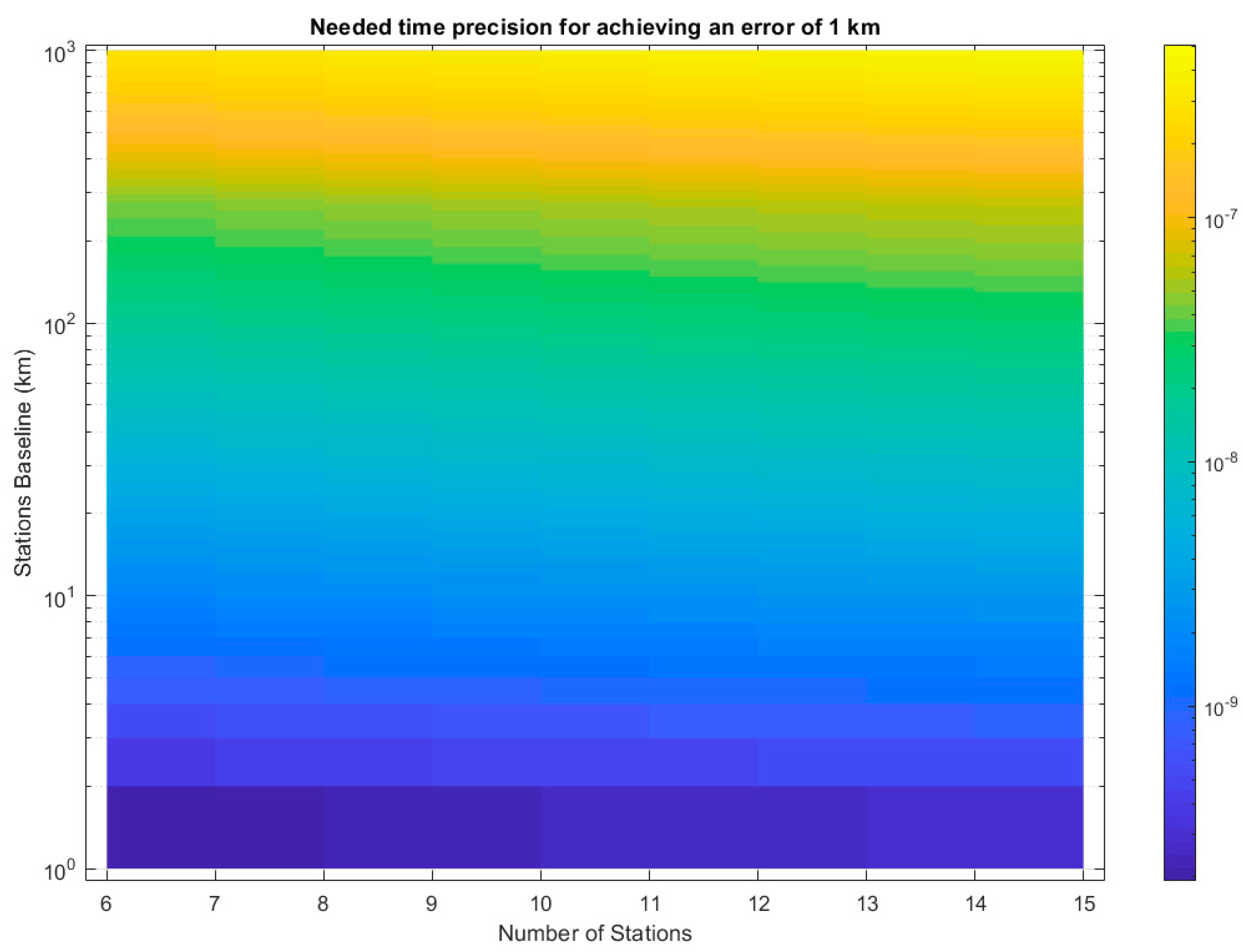
Another convenient utilization of the MDOP is brought by inverting its derivation equation in order to determine the needed performance (in terms of timer error standard deviation of the single sensors) from the single stations. By fixing a target accuracy of 1 km, the needed time precision from every sensor of the network is shown in Figure 11.
For shorter baselines (lower than 50 km), the network needs extremely high accuracy (around 10 ns or lower) for achieving positioning within 1 km. An accuracy around 100 ns is sufficient when considering large baselines, between 200 and 300 km depending on the number of stations. This typology of maps could become extremely helpful in the design phase of a network, in order to set up the baseline and number requirements prior to the discussion of the placement of the stations, which could or could not support a circular network, depending on the area.
5. Conclusions
Time Difference of Arrival networks could support the tracking and orbit determination of spacecraft, launcher and suborbital vehicles. TDOA is based on a distributed network of sensors assigning a timestamp to each received signal from the target. From the evaluation of the differences in the reception times, it is possible to retrieve the position of the target. The geometry of the TDOA network has some peculiarities with respect to the usual implementation of TDOA and hyperbolic tracking methods, mainly relying on the relative position of the receiving stations with respect to the tracked object. The dilution of precision (DOP) is a potentially efficient parameter to be used for the estimation of the network performance, but its value depends on the specific position of the tracked object, while a general performance parameter for the network, by evaluating all the possible angular positions of the target in the celestial vault, should be taken into account. The minimum DOP (MDOP) parameter is derived by comparing the predicted error (by the DOP model) with the mean error achieved through Monte Carlo simulations. The MDOP equals five times the minimum value of DOP registered during the object tracking in all the azimuth and elevation combinations and at a fixed orbit altitude. This value approximates efficiently the mean error when multiplied for the speed of light and the time precision of the sensors. Being dependent on the implementation of a linear least square solution for TDOA positioning, the MDOP coefficient describes the worst case scenario performance of the analyzed networks, so as to simulate the implementation of low-cost sensors and low-calculus power data processors for position calculation. With respect to what is shown by the MDOP, precision can be improved up to the theoretical maximum described by the Cramer−Rao lower bound.
The evaluation of the MDOP trend with respect to parameters such as the stations’ baseline (when considering circular configurations of ground-based stations), target altitude and number of stations has been computed. The MDOP does not appear dependent on the target altitude, while it strongly depends on the stations’ baseline and presents a lower impact related to the number of stations. Indeed, MDOP decreases by approximately one order of magnitude for each order of magnitude increase of the baseline (in km), and it decreases approximately by a factor of two for every 10 additional stations deployed.
Therefore, the baseline appears to be much more impactive on the MDOP decrease than the number of stations. Among the different configurations of networks analyzed in the paper, the most promising is the circle configuration without any sensors located at the circle center. The derivation of the MDOP can be used either for evaluating specific geometries of TDOA stations (an example of two possible configurations of stations in Italy is presented in the work) or for preliminary considerations on the networks to be implemented (with MDOP map, for example, with respect to number of stations and distance and by calculating the needed time precision of the sensors for a target mean localization precision).
Author Contributions
The analyses presented in this paper have been carried out by P.M., while F.S. and F.P. have supervised the research and paper writing. All authors have read and agreed to the published version of the manuscript.
Funding
This research received no external funding.
Acknowledgments
The authors acknowledge the support received by the Italian Space Agency in the framework of the IKUNS (Italian-Kenyan University Nano-Satellites) Programme (within the agreement “Accordo IKUNS-Italian/Kenyan University Nanosatellites—n.2015-031R.1-2018”) for the publication of this paper, whose study is aimed at implementing networks of RF-based and light-based sensors networks for spacecraft tracking and navigation.
Conflicts of Interest
The authors declare no conflict of interest.
References
- McDowell, J.C. The Low Earth Orbit Satellite Population and Impacts of the SpaceX Starlink Constellation. Astrophys. J. Lett. 2020, 892, L36. [Google Scholar] [CrossRef] [Green Version]
- Santoro, F.; Del Bianco, A.; Viola, N.; Fusaro, R.; Albino, V.; Binetti, M.; Marzioli, P. Spaceport and Ground Segment assessment for enabling operations of suborbital transportation systems in the Italian territory. Acta Astronaut. 2018, 152, 396–407. [Google Scholar] [CrossRef]
- Bonnal, C.; Francillout, L.; Moury, M.; Aniakou, U.; Dolado Perez, J.-C.; Mariez, J.; Michel, S. CNES technical considerations on space traffic management. Acta Astronaut. 2020, 167, 296–301. [Google Scholar] [CrossRef]
- Sciré, G.; Santoni, F.; Piergentili, F. Analysis of orbit determination for space based optical space surveillance system. Adv. Space Res. 2015, 56, 421–428. [Google Scholar] [CrossRef]
- Geeraert, J.L.; McMahon, J.W.; Jones, B.A. Orbit determination observability of the dual-satellite geolocation system with TDOA and FDOA. In Proceedings of the AIAA/AAS Astrodynamics Specialist Conference, Long Beach, CA, USA, 13–16 September 2016. [Google Scholar] [CrossRef]
- Hadji Hossein, S.; Acernese, M.; Cardona, T.; Cialone, G.; Curianò, F.; Mariani, L.; Marini, V.; Marzioli, P.; Parisi, L.; Piergentili, F.; et al. Sapienza Space debris Observatory Network (SSON): A high coverage infrastructure for space debris monitoring. J. Space Saf. Eng. 2019, 7, 30–37. [Google Scholar] [CrossRef]
- Chestnut, P.C. Emitter Location Accuracy Using TDOA and Differential Doppler. IEEE Trans. Aerosp. Electron. Syst. 1982, 2, 214–218. [Google Scholar] [CrossRef]
- Guo, F.C.; Fan, Y. A method of dual-satellites geolocation using TDOA and FDOA and its precision analysis. J. Astronaut. 2008, 29, 1381–1386. [Google Scholar]
- Dersan, A.; Tanik, Y. Passive Radar Localization by Time Difference of Arrival; IEEE: Piscataway, NJ, USA, 2002; Volume 2, pp. 1251–1257. [Google Scholar]
- Marzioli, P.; Frezza, L.; Amadio, D.; Santoro, F.; Romanelli, C.; Piergentili, F.; Santoni, F. Innovative tracking systems test on-board a stratospheric balloon: The STRAINS Experiment (paper code IAC-19,B2,4,8,x53632). In Proceedings of the 70th International Astronautical Congress (IAC), Washington, DC, USA, 21–25 October 2019. [Google Scholar]
- Díez-González, J.; Álvarez, R.; Prieto-Fernández, N.; Perez, H. Local Wireless Sensor Networks Positioning Reliability under Sensor Failure. Sensors 2020, 20, 1426. [Google Scholar] [CrossRef] [PubMed] [Green Version]
- Carotenuto, R.; Merenda, M.; Iero, D.; Della Corte, F.G. Mobile Synchronization Recovery for Ultrasonic Indoor Positioning. Sensors 2020, 20, 702. [Google Scholar] [CrossRef] [PubMed] [Green Version]
- Stefański, J. Hyperbolic Position Location Estimation in the Multipath Propagation Environment. In Wireless and Mobile Networking, Proceedings of the Joint IFIP Wireless and Mobile Networking Conference, Gdańsk, Poland, 9–11 September 2009; Wozniak, J., Konorski, J., Katulski, R., Pach, A.R., Eds.; Springer: Berlin/Heidelberg, Germany, 2009; pp. 232–239. [Google Scholar]
- Khalaf-Allah, M. Performance Comparison of Closed-Form Least Squares Algorithms for Hyperbolic 3-D Positioning. J. Sens. Actuator Netw. 2020, 9, 2. [Google Scholar] [CrossRef] [Green Version]
- International Telecommunication Union, ITU Spectrum Management. Available online: https://www.itu.int/pub/R-REP-SM (accessed on 31 August 2020).
- International Telecommunication Union, ITU. ITU Handbook: Mobile-Satellite Service (MSS) 2002; ITU: Geneva, Switzerland, 2002. [Google Scholar]
- International Amateur Radio Union, IARU. Amateur Radio Satellite Frequency Coordination. 2020. Available online: https://www.iaru.org/reference/satellites/ (accessed on 31 August 2020).
- di Palo, L.; Garofalo, R.; Bedetti, E.; Celesti, P.; Iovanna, F.; Frezza, L.; Marzioli, P.; Piergentili, F.; Volpe, A.; Curianò, F.; et al. Time Difference of Arrival for stratospheric balloon tracking: Design and development of the STRAINS Experiment. In Proceedings of the 2020 IEEE 7th International Workshop on Metrology for AeroSpace (MetroAeroSpace), Pisa, Italy, 22–24 June 2020; pp. 362–366. [Google Scholar]
- Marzioli, P.; Frezza, L.; Curianò, F.; Pellegrino, A.; Gianfermo, A.; Angeletti, F.; Arena, L.; Cardona, T.; Valdatta, M.; Santoni, F.; et al. Experimental validation of VOR (VHF Omni Range) navigation system for stratospheric flight. Acta Astronaut. 2021, 178, 423–431. [Google Scholar] [CrossRef]
- Di Palo, L.; Bandini, V.; Bedetti, E.; Broggi, G.; Collettini, L.; Celesti, P.; Di Ienno, D.; Garofalo, R.; Iovanna, F.; Mattei, G.; et al. VOR (VHF Omnidirectional Range) Based Attitude and Position Determination System on a Stratospheric Balloon: TARDIS Experiment; IEEE: Turin, Italy, 2019. [Google Scholar]
- Chen, Y.-H.; Juang, J.-C.; Seo, J.; Lo, S.; Akos, D.M.; Lorenzo, D.S.; Enge, P. Design and implementation of real-time software radio for anti-interference GPS/WAAS sensors. Sensors 2012, 12, 13417–13440. [Google Scholar] [CrossRef] [PubMed] [Green Version]
- Menchinelli, A.; Ingiosi, F.; Pamphili, L.; Marzioli, P.; Patriarca, R.; Costantino, F.; Piergentili, F. A Reliability Engineering Approach for Managing Risks in CubeSats. Aerospace 2018, 5, 121. [Google Scholar] [CrossRef] [Green Version]
- Cavaleri, A.; Motella, B.; Pini, M.; Fantino, M. Detection of Spoofed GPS Signals at Code and Carrier Tracking Level; IEEE: Piscataway, NJ, USA, 2010. [Google Scholar]
- Fernández-Prades, C.; Presti, L.L.; Falletti, E. Satellite radiolocalization from GPS to GNSS and beyond: Novel technologies and applications for civil mass market. Proc. IEEE 2011, 99, 1882–1904. [Google Scholar] [CrossRef]
- Abdul-Latif, O.; Shepherd, P.; Pennock, S. TDoA/AoA Data Fusion for Enhancing Positioning in an Ultra Wideband System; IEEE: Piscataway, NJ, USA, 2007; pp. 1531–1534. [Google Scholar]
- Sarwar, U.; Cheema, K.; Reid, T. Contabat: Designing and Prototyping an Attachable Sports Analytics Device that Provides Ball-Bat Impact Location for Performance Enhancement; American Society of Mechanical Engineers: New York, NY, USA, 2019; Volume 7. [Google Scholar]
- MacCurdy, R.; Gabrielson, R.; Spaulding, E.; Purgue, A.; Cortopassi, K.; Fristrup, K. Automatic animal tracking using matched filters and time difference of arrival. J. Commun. 2009, 4, 487–495. [Google Scholar] [CrossRef] [Green Version]
- Weiser, A.W.; Orchan, Y.; Nathan, R.; Charter, M.; Weiss, A.J.; Toledo, S. Characterizing the Accuracy of a Self-Synchronized Reverse-GPS Wildlife Localization System; IEEE: Piscataway, NJ, USA, 2016. [Google Scholar]
- Bard, J.D.; Ham, F.M. Time difference of arrival dilution of precision and applications. IEEE Trans. Signal Process. 1999, 47, 521–523. [Google Scholar] [CrossRef]
- Kaplan, E.; Hegarty, C. Understanding GPS: Principles and Applications. In Artech House Mobile Communications Series, 2nd ed.; Kaplan, E.D., Hegarty, C., Eds.; Artech House: Boston, MA, USA, 2006; ISBN 978-1-58053-894-7. [Google Scholar]
- Cakir, O.; Yazgan, A.; Kaya, I. Accuracy comparison of time difference of arrival based source localization methods. In Proceedings of the 2015 38th International Conference on Telecommunications and Signal Processing (TSP), Prague, Czech Republic, 9–11 July 2015; pp. 1–4. [Google Scholar]
- Chan, Y.T.; Ho, K.C. A simple and efficient estimator for hyperbolic location. IEEE Trans. Signal Process. 1994, 42, 1905–1915. [Google Scholar] [CrossRef] [Green Version]
- Fiorentin, P.; Bettanini, C.; Bogoni, D. Calibration of an autonomous instrument for monitoring light pollution from drones. Sensors 2019, 19, 5091. [Google Scholar] [CrossRef] [PubMed] [Green Version]
- Wu, P.; Su, S.; Zuo, Z.; Guo, X.; Sun, B.; Wen, X. Time Difference of Arrival (TDoA) Localization Combining Weighted Least Squares and Firefly Algorithm. Sensors 2019, 19, 2554. [Google Scholar] [CrossRef] [PubMed] [Green Version]
Figure 1.
Graphical representation of the variables and factors that will be influencing the dilution of precision (DOP) and minimum dilution of precision (MDOP) values in the paper. Plot (a) shows the top view, plot (b) shows the side view.
Figure 1.
Graphical representation of the variables and factors that will be influencing the dilution of precision (DOP) and minimum dilution of precision (MDOP) values in the paper. Plot (a) shows the top view, plot (b) shows the side view.
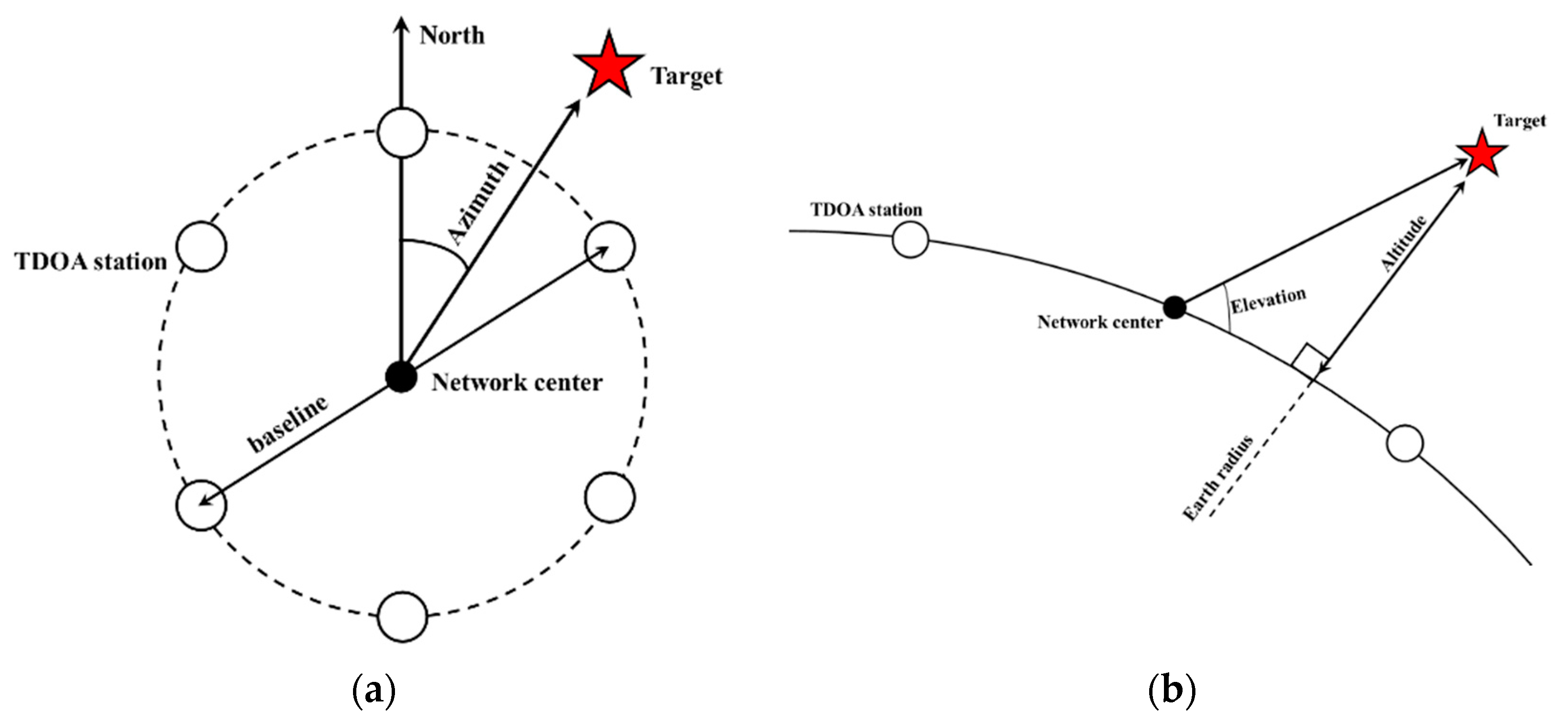
Figure 2.
Example DOP map for a 550 km high satellite, stations located on a circle at 100 km of distance.
Figure 2.
Example DOP map for a 550 km high satellite, stations located on a circle at 100 km of distance.

Figure 3.
DOP trend with respect to elevation (for different baseline values).

Figure 4.
Trend of the two coefficients kAVERAGE and kMIN versus baseline.

Figure 5.
Logarithmic plot of the mean and predicted error plots at different values of the baseline. The “k” coefficient expresses the proportionality coefficient to be decided.
Figure 5.
Logarithmic plot of the mean and predicted error plots at different values of the baseline. The “k” coefficient expresses the proportionality coefficient to be decided.

Figure 6.
Logarithmic plot of MDOP trend for a six station network versus baseline.
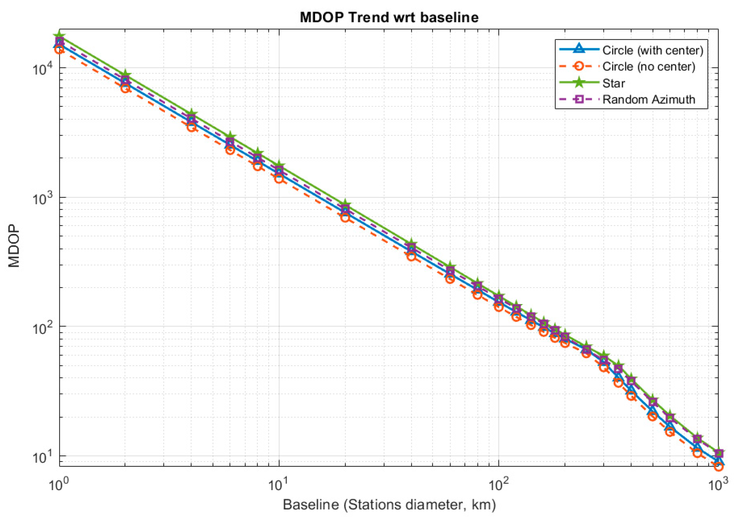
Figure 7.
MDOP trend versus target altitude at different baseline values.
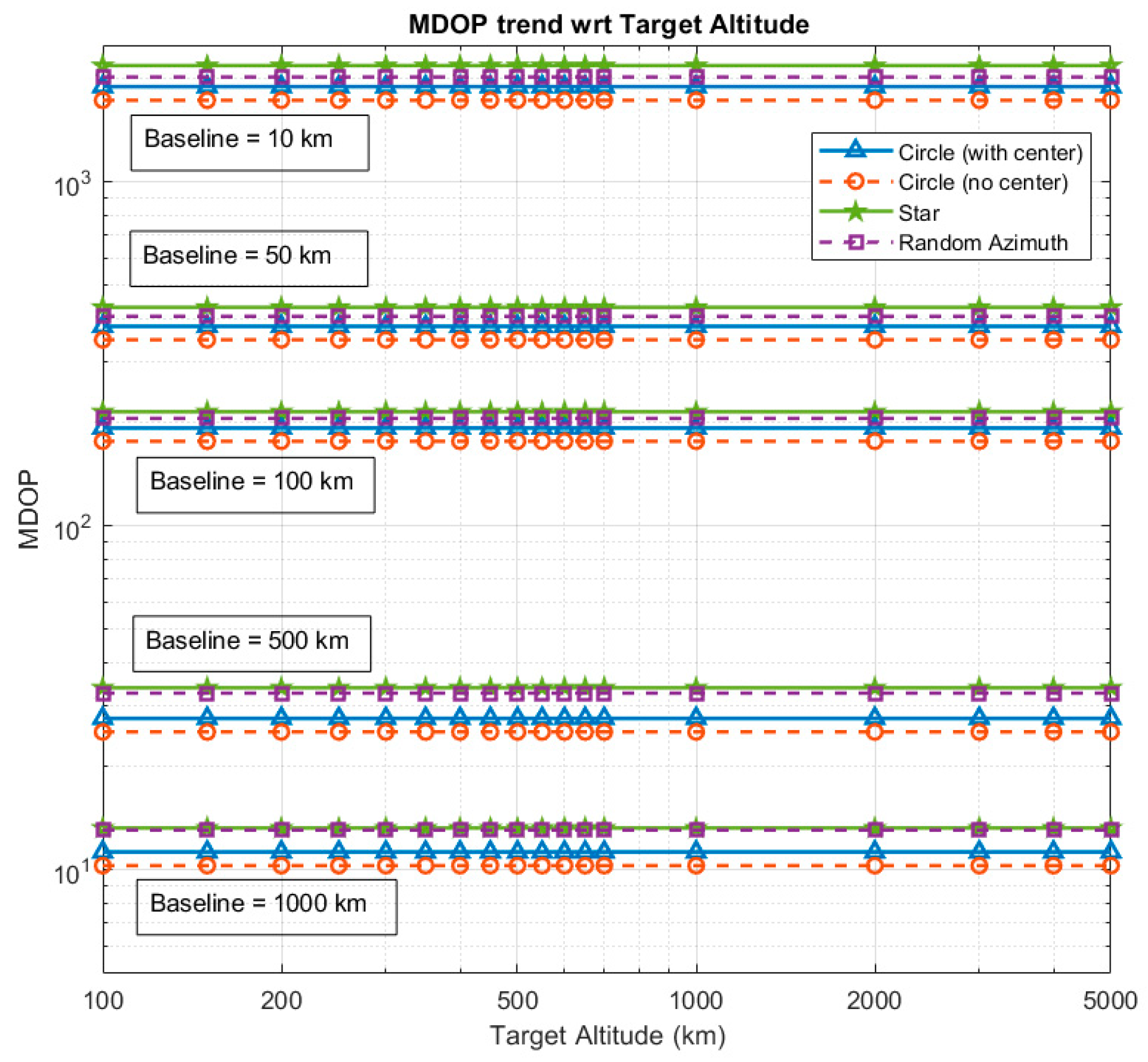
Figure 8.
Logarithmic plot of the MDOP versus the number of stations. The plot is presented for all the selected configurations and for different values of the baseline.
Figure 8.
Logarithmic plot of the MDOP versus the number of stations. The plot is presented for all the selected configurations and for different values of the baseline.
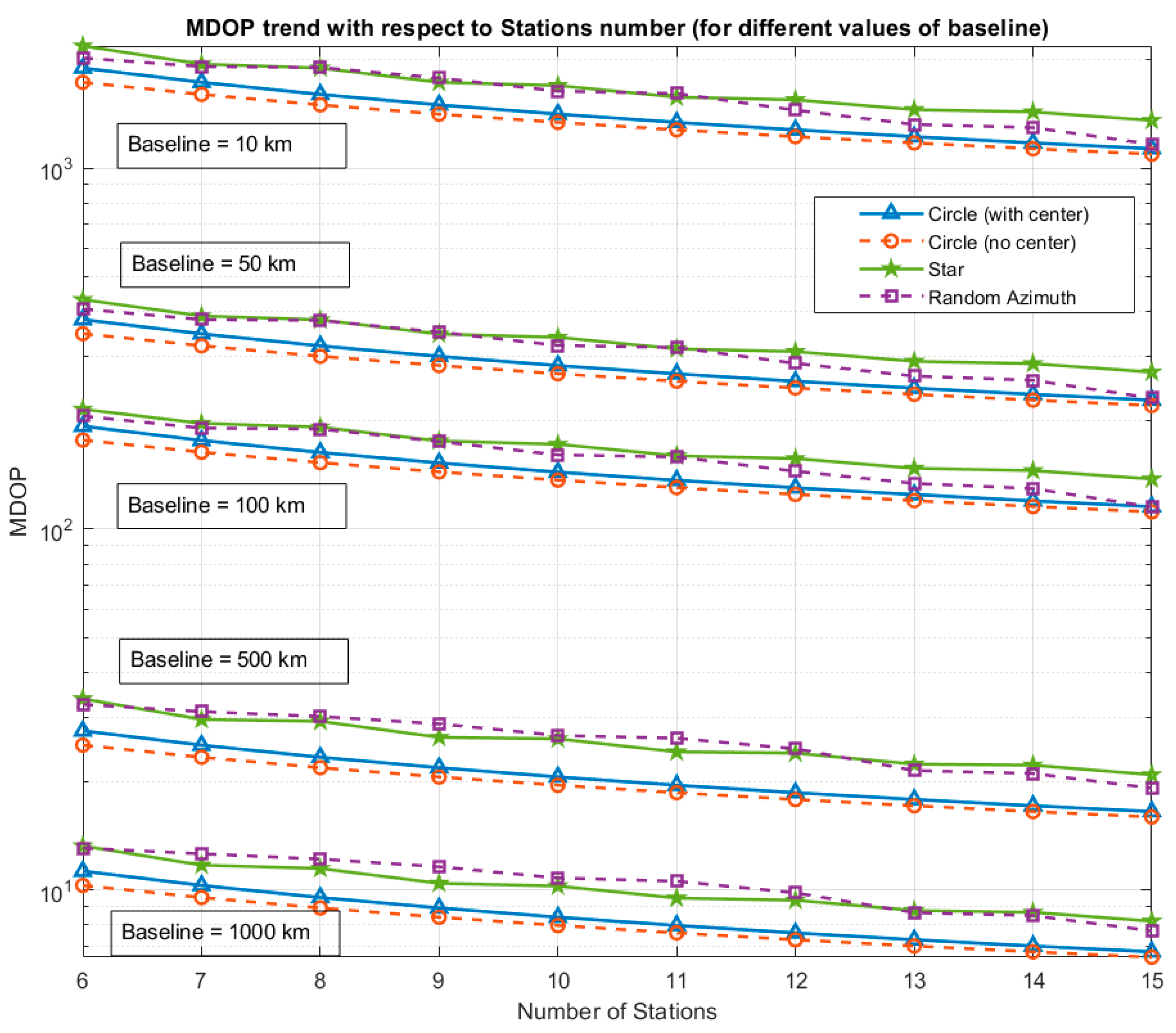
Figure 9.
Example Time Difference of Arrival (TDOA) network configurations to be evaluated. Plot (a) shows Configuration 1, plot (b) shows Configuration 2.
Figure 9.
Example Time Difference of Arrival (TDOA) network configurations to be evaluated. Plot (a) shows Configuration 1, plot (b) shows Configuration 2.
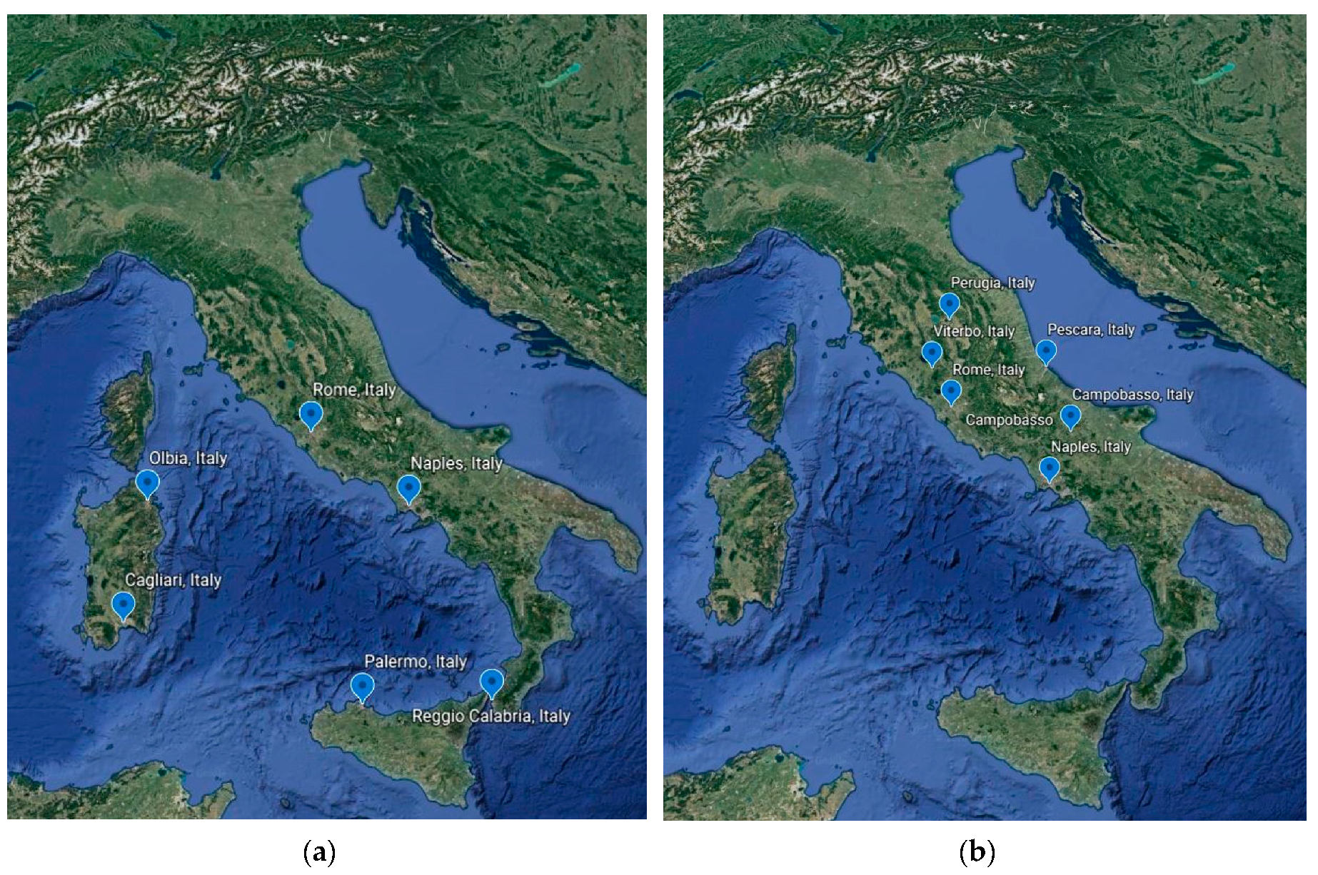
Figure 10.
MDOP value with respect to number of stations and baseline.

Figure 11.
Needed time precision to achieve an accuracy of 1 km in the TDOA position determination.
Publisher’s Note: MDPI stays neutral with regard to jurisdictional claims in published maps and institutional affiliations. |
© 2020 by the authors. Licensee MDPI, Basel, Switzerland. This article is an open access article distributed under the terms and conditions of the Creative Commons Attribution (CC BY) license (http://creativecommons.org/licenses/by/4.0/).
Share and Cite
MDPI and ACS Style
Marzioli, P.; Santoni, F.; Piergentili, F. Evaluation of Time Difference of Arrival (TDOA) Networks Performance for Launcher Vehicles and Spacecraft Tracking. Aerospace 2020, 7, 151. https://doi.org/10.3390/aerospace7100151
AMA Style
Marzioli P, Santoni F, Piergentili F. Evaluation of Time Difference of Arrival (TDOA) Networks Performance for Launcher Vehicles and Spacecraft Tracking. Aerospace. 2020; 7(10):151. https://doi.org/10.3390/aerospace7100151
Chicago/Turabian StyleMarzioli, Paolo, Fabio Santoni, and Fabrizio Piergentili. 2020. "Evaluation of Time Difference of Arrival (TDOA) Networks Performance for Launcher Vehicles and Spacecraft Tracking" Aerospace 7, no. 10: 151. https://doi.org/10.3390/aerospace7100151
Note that from the first issue of 2016, this journal uses article numbers instead of page numbers. See further details here.