Article

Constructive Aerodynamic Interference in a Network of Weakly Coupled Flutter-Based Energy Harvesters

by
Emmanuel Beltramo
1,†,
Martín E. Pérez Segura
1,†,
Bruno A. Roccia
2,†,
Marcelo F. Valdez
3,†,
Marcos L. Verstraete
2,† and
Sergio Preidikman
1,*,†
1
Instituto de Estudios Avanzados en Ingeniería y Tecnología (IDIT), Universidad Nacional de Córdoba—CONICET, Córdoba 5000, Córdoba, Argentina
2
Grupo de Matemática Aplicada, Facultad de Ingeniería, Universidad Nacional de Río Cuarto, Río Cuarto, Córdoba X5804BYA, Argentina
3
Facultad de Ingeniería and Instituto de Investigaciones en Energía no Convencional (INENCO), Universidad Nacional de Salta—CONICET, Salta 4400, Salta, Argentina
*
Author to whom correspondence should be addressed.
These authors contributed equally to this work.
Aerospace 2020, 7(12), 167; https://doi.org/10.3390/aerospace7120167
Submission received: 21 October 2020 / Revised: 14 November 2020 / Accepted: 20 November 2020 / Published: 24 November 2020
(This article belongs to the Special Issue Aeroelasticity, Volume II)

Abstract

:
Converting flow-induced vibrations into electricity for low-power generation has received growing attention over the past few years. Aeroelastic phenomena, good candidates to yield high energy performance in renewable wind energy harvesting (EH) systems, can play a pivotal role in providing sufficient power for extended operation with little or no battery replacement. In this paper, a numerical model and a co-simulation approach have been developed to study a new EH device for power generation. We investigate the problem focusing on a weakly aerodynamically coupled flutter-based EH system. It consists of two flexible wings anchored by cantilevered beams with attached piezoelectric layers, undergoing nonlinear coupled bending–torsion limit cycle oscillations. Besides the development of individual EH devices, further issues are posed when considering multiple objects for realizing a network of devices and magnifying the extracted power due to nonlinear synergies and constructive interferences. This work investigates the effect of various external conditions and physical parameters on the performance of the piezoaeroelastic array of devices. From the viewpoint of applications, we are most concerned about whether an EH can generate sufficient power under a variable excitation. The results of this study can be used for the design and integration of low-energy wind generation technologies into buildings, bridges, and built-in sensor networks in aircraft structures.

1. Introduction

The energy harvesting concept is related to the small-scale energy extraction of various sources, usually by means of unconventional mechanisms. For example, the unavoidable random mechanical vibrations of a structure, such as a building, a bridge, or an aircraft wing, may be transformed into an electrical signal with a properly designed transducer. Depending on the application, this electrical signal could potentially replace small batteries to power small devices, such as wireless sensors and transmitters for health monitoring, microelectromechanical (MEM) devices, low maintenance, and hard-to-access actuators, to mention a few examples.
Rather than feeding on the vibrations of existing systems, a popular option for wind energy harvesting relies on external devices, harvesters, especially designed to exploit one or more fluid-interaction phenomena. Among the most popular aeroelastic phenomena considered are vortex-induced vibrations, galloping, buffeting, and flutter.
Although the body of research on this field is continuously growing, the technology of wind energy harvesting is still far from mature to be 100% reliable. There are still open challenges that need to be addressed, the low power output being one of the most recurring.
The driving question of the present effort is: Can the energy harvesting ability (cut-in speed and power output) be enhanced through constructive aerodynamic interactions between multiple flutter-based harvesters? To the best of the authors’ knowledge, there is no comprehensive study, neither numerical nor experimental, on three-dimensional arrays of flutter-based cantilever harvesters in cross-flow. Thus, the aim of this article is to help fill in this research gap. In the end, a numerical analysis of an array of two low-aspect-ratio flutter-based harvesters in cross-flow, the first of its kind, is presented. The analysis undertaken is novel not only because it is based on a fully three-dimensional model but also because it uncovers a new realm of possibilities for harvesting energy at lower, more approachable wind speeds.
The computational framework developed and used in the present study involves coupled mechanical, piezoelectric, and aerodynamic systems. The aerodynamic model is based on the Unsteady Vortex Lattice Method (UVLM) for the solution of the incompressible and irrotational flow around the immersed bodies. The three-dimensional structure is modeled as a modified Euler–Bernoulli beam, which can accommodate embedded piezoelectric layers along all or part of its length.

Aeroelastic Energy Harvesting

A flexible body immersed in a fluid flow can experience oscillations as a consequence of interactions between inertial, elastic, dissipative, control, and aerodynamic forces [1]. Among the different aeroelastic phenomena, flutter has been extensively studied and pinpointed as the cause of many catastrophic civil and aeronautical events. A relatively recent research stream has focused on exploiting this nonlinear fluid–solid interaction phenomenon to produce electricity at a small scale [2], establishing the field of energy harvesting based on aeroelastic flutter (EHAF). Examples of such efforts exploring different designs of harvester devices can be found in [3,4,5,6,7,8,9]. One of the options to harvest energy from a flexible structure in a postcritical flutter response is to use piezoelectric materials. The embedded piezoelectric layers generate an electric voltage proportional to their deformation. Therefore, the deformation of the structure is transformed into an electrical signal that can be used as an electric energy source.
The risks, potentialities, and opportunity costs of EHAF technology can be assessed by means of nonlinear aeroelasticity analysis [10,11]. The flutter response of a system is generally dependent on a combination of several sources of nonlinearities: aerodynamics, material behavior, geometrical, structural coupling, free-play, and so on. These nonlinearities may lead to a different realm of dynamical behaviors, including bifurcations, limit cycle oscillations (LCO), chaos, and various types of resonances (internal and super/subharmonic). Along these lines, several seminal works that explore nonlinear torsional and flexural stiffness ([12,13]), free-play and cubic stiffness ([10,14,15]), stall flutter ([16,17]), and system parameter uncertainties [18] have been published to date. Most of these studies are numerical and deal with simplified bidimensional models specially tailored to quantify the effect of a particular parameter on the extracted electrical power.
Despite the progress in recent years, most of the studies in the literature were only able to produce limited power outputs, ranging from few microwatts ([3,4,5,6,11,14,19]) to tenths of watts ([17,20]). Some recent experimental and numerical studies ([21,22]) were able to show power outputs close to 7 milliwatts by exploiting the flag-flutter phenomenon through piezoelectric materials. The power limitation concern has prompted new designs involving tuning strategies ([23,24]), interference phenomena ([25,26]), hybrid systems using multiple physical phenomena ([27,28]), adaptive mechanisms [29], and multiple harvesters in different configurations ([30,31,32,33]) in order to ramp up the power output. Zhu et al. [23] reviewed several strategies to increase the operational frequency range of vibration-based harvesters. Some of the options are: resonant frequency tuning, bandwidth widening, intermittent and continuous tuning, and the use of nonlinear springs and bistable structures, among others. Hafezi and Mirdamadi [29] proposed a novel adaptive mechanism to displace a point mass along a piezoelectric beam. The change of the inertial properties of the harvester implies a wider flutter region and, in turn, more energy extraction.
In the context of multiple harvesters, Bryant et al. [30] provided novel insights on the effect of aerodynamic interference on the conversion efficiency of an array of harvesters. They showed that the amplitude and frequency of oscillation of a harvester, hence its power output, are significantly impacted by the interaction of this harvester with the vortical wake of an upstream device/harvester. Deivasigamani et al. [32] experimentally observed a 20% to 40% increase in the power output of the downstream harvester in a two-harvester tandem array aligned with the wind direction. On the same line, McCarthy et al. [31] studied two piezoelectric harvesters in tandem through experimental flow visualization and voltage data analysis. They observed that the leading-edge wake of the upstream harvester has a negligible impact on the power output of the downstream harvester. However, its trailing edge wake does produce an amplification of the power output. Recently, Kirschmeier and Bryant [34] experimentally investigated the effect of structural parameters on the aerodynamic coupling between two devices in a tandem configuration. They showed that the limit cycle and transient response of the downstream wing depend heavily on its own pitch stiffness. On the other hand, the aeroelastic stability and flutter point of the downstream wing is dictated by the upstream wing. Roccia et al. [33] proposed a two-dimensional computational model for predicting the piezoaeroelastic response of vertically arranged harvesters. They showed that the flutter region of the two-harvester system could be significantly extended by tuning the separation between them. Their results suggest that it is possible to extract energy at low airspeeds and improve the power output during the postcritical regime.
Despite the promising results, the use of harvesters arrays as a technological solution to the problem of the low power output of piezoelectric–aeroelastic systems has posed through another set scarcely explored challenges: effect of the spatial configuration of harvesters [35] (aerodynamic shadow interference) and wake–harvester interactions on the overall power output, effect of structural/mechanical/electrical coupling between harvesters, nonlinear synchronization phenomena, and so on.
The article is outlined as follows. In Section 2, the aerodynamic model (Section 2.1), structural model (Section 2.2), coupling strategy (Section 2.3) are presented. In Section 3, the results are presented. First, a verification study (Section 3.1) is performed to compare the predictions of the current framework with values reported in the literature. Finally, in Section 3.2, the main study of this article on the flutter and postcritical response of an array of two vertically aligned piezoelectric harvesters is presented.

2. Materials and Methods

In the following sections, the different components of the computational framework are presented. First, the aerodynamic model and the Unsteady Vortex Lattice Method is succinctly described. Next, the structural model and finite-element discretization are discussed. Finally, the coupling technique between these physics is laid out.

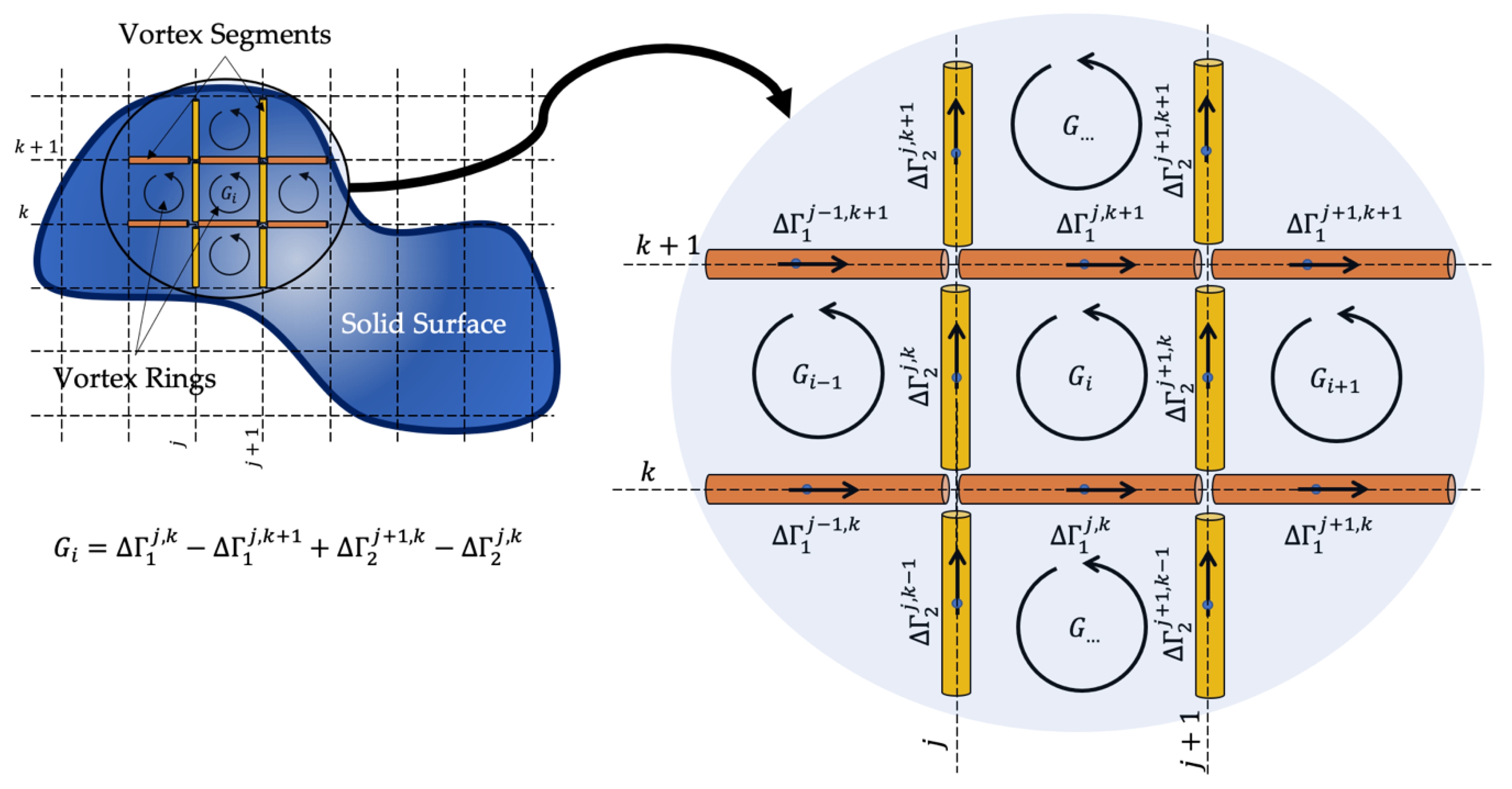
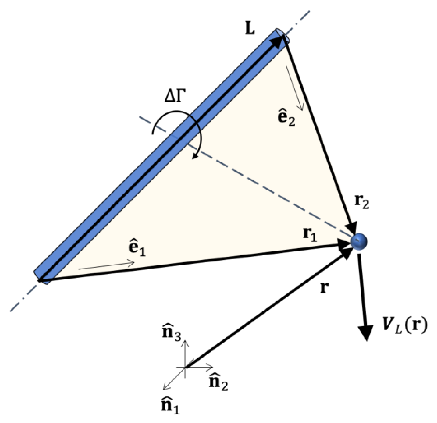
2.1. Aerodynamic Model

The main purpose of the aerodynamic model in the present framework is to provide an estimate of the aerodynamic loads. The well-known Unsteady Vortex Lattice Method (UVLM) was chosen for this purpose because it constitutes a trade-off between desired precision and computational cost compared to other flow solvers based on computational fluid dynamics (CFD) techniques such as Reynolds Average Navier–Stokes (RANS), Large Eddy Simulation (LES), Direct Numerical Simulation (DNS), and so on.
The UVLM is based on the premises of incompressible and irrotational flow outside the compact vorticity containing regions: boundary layers adjacent to the solid boundaries and wakes. In real flows at moderate to high Reynolds numbers, boundary layers develop adjacent to the surfaces of the bodies. Enough vorticity is present in this layer to smoothly build up the flow velocity from zero at the surface (no-slipping condition) to the outer flow condition. As the Reynolds number increases, the thickness of the boundary layer decreases due to the progressive reduction of the influence of viscous diffusion relative to convective linear momentum transport. In the limit of infinite Reynolds number, the boundary layers (and other regions containing vorticity) become extremely thin but still enclose enough vorticity to produce the velocity transition from no-slip to outer flow conditions. In fact, in this situation, the boundary layers appear to produce an almost discontinuous jump in the tangential velocity of the flow, resembling the ideal scenario of an infinitesimally thin vortex sheet. Two types of vortex sheets are recognized: bound vortex sheets modeling the boundary layers attached to the solid boundaries B and free-vortex sheets representing the wakes F . For problems involving N B bodies, the solid boundaries B i are collectively represented by B = i = 1 N B B i . Similarly, all N F vortex sheets are collectively represented by F = i = 1 N F F i . The bound vortex sheets move with the bodies; as a result, a finite pressure jump develops across them. Conversely, the free-vortex sheets grow and deform freely to attain force-free positions. The two types of vortex sheets merge at the points of the bodies where flow separation occurs. In this effort, it is assumed that the immersed bodies (harvesters) are very thin; therefore, the vortex sheets on both sides of the body effectively collapse into one.
The flow outside the vortex sheets is incompressible and irrotational; hence, a velocity potential Ψ exists and satisfies the Laplace equation (continuity for incompressible, irrotational flows):
2 Ψ = 0 .
The velocity field V ( r ; t ) = Ψ must satisfy at all times the no-penetration condition on the surface B of the bodies:
( V ( r ; t ) V S ( r ; t ) ) n ^ ( r ; t ) = 0   r B ,
where n ^ ( r ; t ) is the unit vector normal to the solid surface at the location r and V S ( r ; t ) is the velocity of the solid surface at r . Additionally, it is required that the perturbations introduced on the flow by the bodies decay to zero far away from them. This regularity condition at infinity is satisfied automatically by the fundamental solutions (vortex, source/sink, dipole) of the Laplace equation. Due to the linearity of the Laplace equation, the fluid velocity anywhere in the flow field can be decomposed into the free-stream component V and the fluid velocity due to the vorticity present on the bound and free-vortex sheet V B and V F , respectively:
V ( r ; t ) = V + V B ( r ; t ) + V F ( r ; t ) .
The last two components can be obtained from the vorticity in the vortex sheets through the Biot–Savart law:
V B ( r ; t ) = 1 4 π B   γ B ( r 0 ; t ) × ( r r 0 ) ( ( r r 0 ) ( r r 0 ) ) 3 2 d S ( r 0 ) ,
V F ( r ; t ) = 1 4 π F   γ F ( r 0 ; t ) × ( r r 0 ) ( ( r r 0 ) ( r r 0 ) ) 3 2 d S ( r 0 ) ,
where d S ( r 0 ) is an infinitesimal surface element and γ ( r 0 , t ) is the vorticity in the vortex sheets. This vorticity is spatially conserved as a consequence of the following kinematic relation:
γ ( r ; t ) = × V ( r ; t ) γ ( r ; t ) = 0 .
Finally, the unsteady Bernoulli’s equation can be used to obtain the pressure distribution on the body surface and the resultant aerodynamic loads. This equation is given by:
p p = ρ 2 ( V V V V ) t ( Φ Φ ) = 0 .
The resultant aerodynamic loads, force, and moment about a pivot point O i acting on each body B i are computed as follows:
F i ( t ) = B i   ( p ( r ; t ) p ) n ^ ( r 0 ; t ) d S ( r 0 ) ,
M O i i ( t ) = B i   ( r r O i ) × n ^ ( r 0 ; t ) ( p ( r ; t ) p ) d S ( r 0 ) .
In the UVLM formulation, the bound vortex sheets attached to each body are discretized with collections of finite-length vortex segments of constant circulation Δ Γ . In order to fulfill the spatial conservation of vorticity (Equation (6)), the vortex segments, in turn, must conform to an array of (ideally four-sided) closed vortex rings with constant circulation (Figure 1). Similarly, the wakes are discretized with vortex segments forming closed vortex rings of constant circulation that automatically satisfy the spatial conservation of vorticity.
A consequence of the discretization is that the no-penetration condition on a body B k can only be satisfied at a finite number M k of collocation points on its solid surface. It can be shown [36] that the contribution to the normal component of the fluid velocity at the location r i k B k of the collocation point i on the body B k due to all the bound vortex sheets can be approximated as follows:
V B k ( r i k ; t ) n ^ ( r i k ; t ) m = 1 N B j = 1 N m G j m ( t ) A i j k m ( t )   i = 1 , 2 , ,   M k
where A i j k m denotes the aerodynamic influence of the j-th vortex ring attached to the body B m over the i-th collocation point on the surface of body B k , G j m is the circulation of the j-th vortex ring attached to the body B m , and N m is the number of bound vortex rings in B m . The influence coefficients A i j k m are obtained by summing up the contributions to the normal component of the fluid velocity at the collocation point i due to the vortex segments (with unitary circulation) that make up the vortex ring j. The velocity due to a vortex segment of length L and unit circulation is given by:
V L ( r ) = 1 4 π L × r 1 L × r 1 2 2 L ( e ^ 1 e ^ 2 ) ,
where quantities L , r 1 , r 2 , e ^ 1 , and e ^ 2 are defined in Figure 2.
It is observed that V L ( r ) blows up when r 1 L ; that is to say, when the point where the velocity is evaluated lies along the direction of the vortex segment. This situation can potentially lead to numerical instabilities when updating the position of the free-vortex segment in the wakes. To avoid such a situation, it is customary to implement a smoothing or cut-off technique. In the current framework, a simple cut-off strategy is used that consists of replacing the denominator in Equation (11) by L × r 1 2 2 + ( δ L ) 2 [37], which effectively adds a finite core to the vortex segment. The no-penetration condition at the collocation point i of body B k is readily expressed as follows:
m = 1 N B j = 1 N m G j m ( t ) A i j k m ( t ) = V S ( r i k ; t ) n ^ ( r i k ; t ) V n ^ ( r i k ; t ) V F n ^ ( r i k ; t ) = RHS i k
It is noted that the contribution of the wakes (free-vortex sheets F ) was moved to the right-hand side of Equation (12). Once generated, the circulation of the free-vortex rings is conserved in time, and the rings move with the local fluid velocity to attain force-free configurations. Therefore, not only is their circulation known but also their location; therefore, their contribution to the fluid velocity on the collocation points is known through the Biot–Savart equation (Equation (5)).
It can be shown that the following algebraic system of equations is obtained upon enforcing the no-penetration condition on all the collocation points on all the bodies:
[   [ A i j 11 ] [ A i j 12 ] [ A i j 1 N B ] [ A i j 21 ] [ A i j 22 ] [ A i j 2 N B ] [ A i j N B 1 ] [ A i j N B 2 ] [ A i j N B N B ] ] { { G j 1 } { G j 2 } { G j N B } } = { { RHS i 1 } { RHS i 2 } { RHS i N B } }
where [ A i j k m ]   M k × N m , { G j m }   N m × 1 , { RHS i k }   M k × 1 , and RHS i k is the normal component of the fluid velocity on the i-th control point of body B k due to all other agents (free current, wakes, body motion, and so on) but the bound vorticity (vortex rings).
In Equation (13), a quasi-steady aerodynamic coupling between the different bodies is captured by the off-diagonal matrix blocks [ A i j k m ] with k m , which account for the bound vorticity interactions (aerodynamic shadow effect) of body B m over body B k . The other unsteady aerodynamic coupling between the bodies is encapsulated in the right-hand side terms RHS in which the effect of the wake of a body over another body is accounted for (Equation (12)).
The free-vortex sheets or wakes are created from the edges of the bodies where flow separation occurs by means of vorticity convection. Flow separation cannot be predicted within an irrotational framework (no-slip condition cannot be enforced) unless a boundary layer model or another more sophisticated strategy is incorporated. In the current effort, no such strategies are implemented. Instead, flow separation is assumed a priori to occur from specified locations, particularly from the trailing edge of streamlined bodies. The flow separation phenomenon is replicated in the current framework by the convection of the vortex segments along the trailing edge of the bodies into the flow field (Figure 3). By Equation (6), the advected vortex segments must also form closed vortex rings, hence they close on the trailing edge through vortex segments parallel to the flow field. Once a part of the wake, the vortex rings move with the local fluid velocity conserving its sectional circulation. The motion of a free-vortex ring is achieved by moving its four corner points with the local fluid velocity. The time stepping is done through the first-order forward Euler scheme as follows:
d r P ( t ) d t = V ( r P ; t ) r P ( t + Δ t ) r P ( t ) + V ( r P ; t ) Δ t

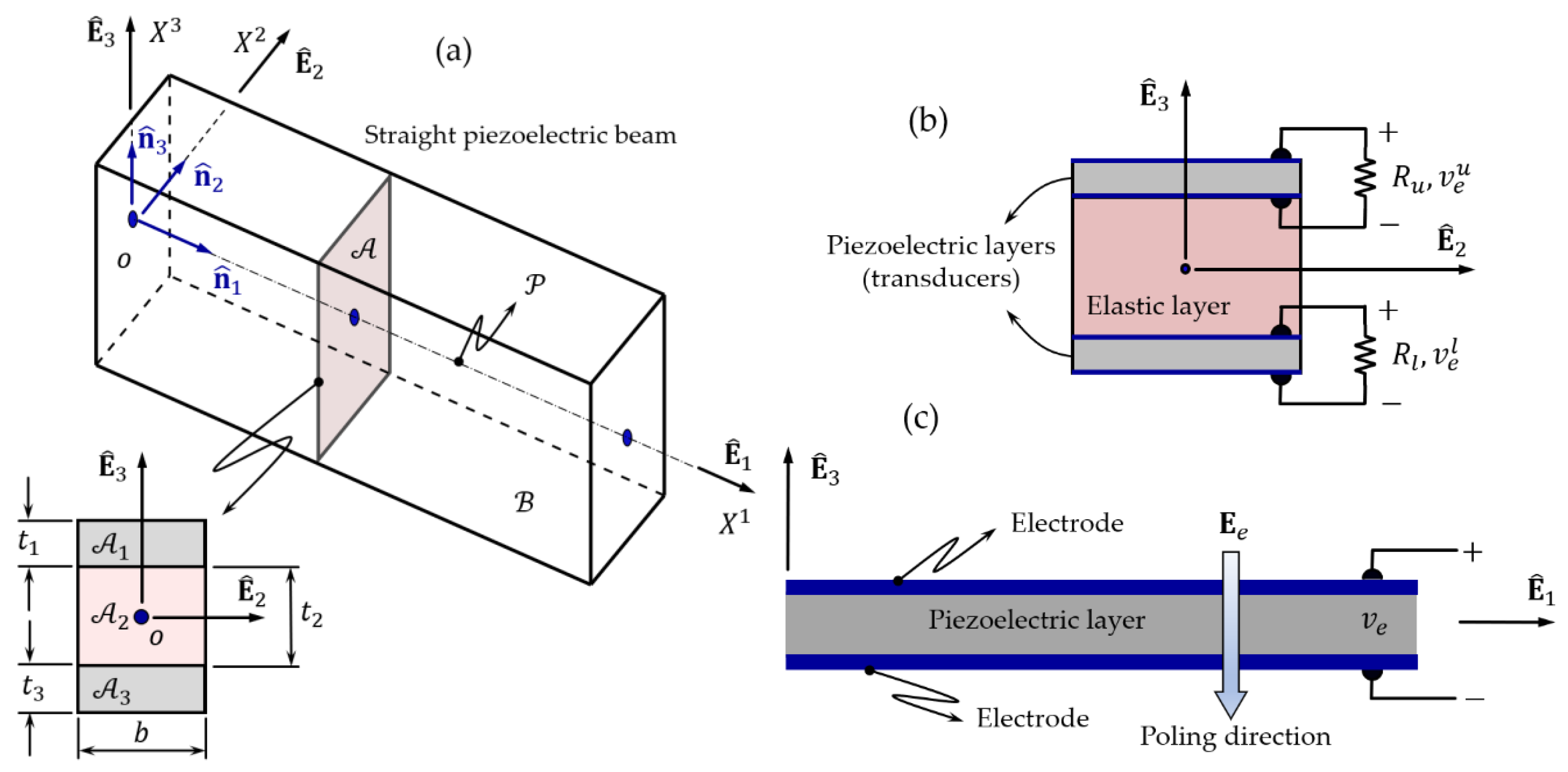
2.2. Structural Model

The main aspects of the structural model are summarized next. The equations of the motion of a finite-element, three-dimensional piezoelectric beam and its associated set of reduced-order equations are presented.
In this effort, the piezoelectric beam studied is composed of an elastic core and two exterior layers of piezoelectric material (transducers) with their respective electrodes. The piezoelectric layers are symmetrically arranged with respect to the bending neutral axis of the section. This beam is depicted schematically in Figure 4a.
The beam reference domain is decomposed as the Cartesian product of the beam axis P and the beam normal cross-section A . The cross-section A is decomposed in three subdomains A i ; that is to say, A = i = 1 3 A i , where A 1 and A 3 are the cross-sections of the piezoelectric layers and A 2 is the cross-section of the elastic layer. Each cross-section A i is rectangular with the same width b and thickness t i (Figure 4a). Each piezoelectric layer is covered by a pair of electrodes on their top and bottom surfaces. These electrodes are assumed to be perfectly conductive and to have negligible mechanical properties (Figure 4c). In addition, the transducers are electrically independent of one another, which means that the coupling between the axial and bending deformations can be accounted for. Therefore, two generalized coordinates, v e u and v e l , are employed for the electric potential difference across the upper and lower piezoelectric layer, respectively. To estimate the power, the electrodes in each layer are connected to the resistors R u and R l , as shown in Figure 4b. This electric configuration has been extensively used in similar studies.
Regarding the material properties, the elastic layer is assumed to be homogeneous and isotropic. On the other hand, the piezoelectric layers are idealized as transversely isotropic materials, with their isotropic plane normal to the poling direction [38].
In this effort, a Rayleigh-like beam element satisfying the following kinematic hypothesis is assumed:
H1. 
The cross-section A remains planar and does not suffer in-plane deformations. This means that in-plane shear strains and Poisson’s effect due to axial strains are assumed negligible;
H2. 
The rotated cross-sections are always orthogonal to the deformed beam axis. This is the well-known Euler–Bernoulli assumption; and
H3. 
The elastic core and the piezoelectric layers are perfectly bonded. This means that the deformation field is continuous across the elastic and piezoelectric layers.
In the description that follows, Latin indices i, j, k, and so on range from 1 to 3, and Greek indices range from 2 to 3. In addition, Einstein’s summation is implied unless otherwise specified.
The body kinematics under deformation are described by means of a reference and the current configurations, and D , respectively, both defined with respect to a global reference frame N = { n ^ 1 , n ^ 2 , n ^ 3 } . In order to describe the reference configuration, a right-handed orthonormal frame = { E ^ 1 , E ^ 2 , E ^ 3 } , called reference frame, is introduced, with an associated set of coordinates ( X 1 , X 2 , X 3 ) . This frame is such that E ^ 2 and E ^ 3 lay on a generic cross-section and E ^ 1 is parallel to the beam axis. The beam reference configuration is described by the position vector R 0 = X i E ^ i . To describe the beam current configuration, another right-handed orthonormal frame e = { e ^ 1 , e ^ 2 , e ^ 3 } , called moving or current frame, is introduced, such that e ^ k = Λ ( X 1 ) E ^ k and Λ ( X 1 ) S O ( 3 ) is a one-parameter rotation tensor. Due to the hypothesis (H1), the position in the deformed configuration of material points lying on an arbitrary cross-section are uniquely specified by the vector R ( X 1 , X 2 , X 3 ) = r ( X 1 ) + X α e ^ α = r ( X 1 ) + Λ ( X 1 ) X [39], where r ( X 1 ) is the position in the current configuration of a point lying on the beam axis and X = X α E ^ α .
In the present effort, only linear beam theory is considered. This means that the components of the displacement vector of a material point on the beam axis u 0 = r ( X 1 ) X 1 E ^ 1 are small compared to the beam length L, and the rotations are small enough so that the rotation tensor can be approximated to the first order by Λ ( X 1 ) 1 + θ ˜ ( X 1 ) [40]. Here, 1 stands for the second-order identity tensor, and θ ˜ is a skew-symmetric tensor whose components can be interpreted as infinitesimal rotations. It can be shown that two successive infinitesimal rotations are independent of the order (commutative property), and thus, they can be regarded as vectors. With these assumptions, the displacement vector field of a generic point belonging to the beam cross-section can be expressed as,
u ( X 1 , X 2 , X 3 ; t ) = u 0 ( X 1 ; t ) + θ ˜ ( 2 , 3 ) ( X 1 ; t ) X ,
where
θ ˜ ( 2 , 3 ) = [ 0 θ 3 ( X 1 ; t ) θ 2 ( X 1 ; t ) θ 3 ( X 1 ; t ) 0 0 θ 2 ( X 1 ; t ) 0 0 ] .
Here, θ 2 ( θ 3 ) denotes the rotation of the cross-section around the E ^ 2 ( E ^ 3 ) axis, and the axial vector associated to θ ˜ ( 2 , 3 ) is given by θ ( 2 , 3 ) = θ α E ^ α . It is recalled at this time that the theory above only relates to the bending motion of the beam, so the rotation about the axis E ^ 1 (torsion) is not included in order to fulfil Euler–Bernoulli hypothesis (H2) [41]. This is equivalent to the assumption that the torsional and bending deformation of the beam are independent (uncoupled). As it is customary in linear 3D beam formulations, the torsion effect is included in an ad-hoc fashion during the finite-element discretization procedure. Thus, a three-dimensional Euler–Bernoulli beam element is obtained, which includes torsion in a completely decoupled way.
From Equation (15), knowing that R = u + R 0 , the deformation gradient tensor F = k ( R ) E ^ k can be computed, where the symbol k ( ) stands for partial derivative with respect to X k and represents the tensor product. The Green–Lagrange strain tensor ε G L can then be computed by means of the displacement gradient tensor F ¯ = F 1 . Neglecting all higher-order strain terms in ε G L , except for the so-called von Kármán nonlinear strains, which involve the squares of 1 u 0 2 and 1 u 0 3 , leads to the following expression of the Green–Lagrange strain tensor [42],
ε G L = ( 1 u 0 + 1 θ ˜ ( 2 , 3 ) X θ ˜ ( 2 , 3 ) E ^ 1 ) E ^ 1 + 1 2 [ ( 1 u 0 2 ) 2 + ( 1 u 0 3 ) 2 ] E ^ 1 E ^ 1 .
Due to the hypothesis (H2), the shear strain components (coordinates of E ^ 1 E ^ 2 and E ^ 1 E ^ 3 ) in Equation (17) must be identically zero. This hypothesis leads to two additional kinematical constraints: θ 2 = 1 u 0 3 and θ 3 = 1 u 0 2 . Furthermore, the term 1 θ ˜ ( 2 , 3 ) , or equivalently, κ = 1 θ α E ^ α , can be recognized as the curvature vector of the beam axis.
The stress–strain constitutive relations for the elastic and piezoelectric layers are assumed to be linearly elastic, i.e., they follow Hooke’s law. In addition, piezoelectric materials generate an electric field when they are deformed; conversely, they suffer deformation when an electric field is applied across them. These phenomena are called direct and converse piezoelectric effects, respectively [38]. The piezoelectric behavior can be described by linear constitutive equations if the electric fields and the mechanical strains are sufficiently small, yielding the following standard form
σ = E e : ε G L ( d m ) T · E e D = d m : ε G L + e m ε · E e ,
where σ is the mechanical stress tensor, D is the electric displacement vector (or electric flux density), E e is the electric vector field, which is related to the electric potential v e as E e = v e , E e is the four-order elasticity tensor evaluated at a constant electric field, d m is the third-order tensor of piezoelectric coefficients, e m ε is the second-order dielectric permittivity tensor evaluated at constant strain field, and the notation “ : ” indicates tensor double-contraction operation. It should be noted that the constitutive relations exposed in Equation (18) reduce to the well-known generalized Hooke’s law σ =   : ε G L for elastic layers when the piezoelectric effect is ignored ( E e 0 ).
As can be observed in Figure 4c, the piezoelectric layer is poled across its thickness. In addition, the electric potential is assumed to vary linearly across the electrode pair, namely, the electric field is uniform along the thickness direction. Therefore, the electric vector field through the i-th piezoelectric layer has only one nonzero component and can be expressed as the voltage-to-thickness ratio E e = ( ± v e / t i ) E ^ 3 .
To obtain the equations of motion for the electromechanical beam introduced above, an extended version of the variational Hamilton’s principle that accounts for piezoelectric media is used [43,44]. There are two alternatives for dealing with the independent electrical variables. The first option is to use the electric charges as independent variables. The second option is to use the flux linkages as the independent variables. In any case, the electric fluxes can be related to the voltage through the constitutive relations of each electrical component. The resulting variational principle may be stated in Mandel’s notation as follows [45],
t 1 t 2 { δ ( 1 2 Ω   ρ u ˙ T u ˙ d Ω ) δ ( 1 2 Ω   ε ¯ T [ C E e ε ¯ d m T E e ] d Ω ) + δ ( 1 2 Ω   D T E e d Ω ) +   δ W ¯ n c } d t = 0 ,
where the over-dots denote time derivatives, ρ is the density of the piezoelectric/elastic layer, ε ¯ 6 is the Mandel representation of the second-order tensor ε G L , C E e 6 × 6 is the Mandel representation of E e , d m 3 × 6 is the Mandel representation of d m , and δ W ¯ n c is the nonconservative virtual work, which in the present effort is done by the fluid forces (Equations (8) and (9)) and by the electric dissipation “forces.” Due to the beam hypotheses adopted, ε ¯ 1 is the only nonzero component of the vector ε ¯ and therefore only C 11 E e is needed. Because of the electric field direction and the assumption of transversely isotropic material for the piezoelectric layers, matrices d m and e m ε are reduced to the scalars ( d m ) 31 and ( e m ε ) 33 , respectively.

Discretized Dynamic Formulation (Finite-Element Model)

The resulting partial differential equations obtained through the generalized Hamilton’s principle are then discretized in the spatial domain by the finite-element method. This technique requires the beam domain to be divided into a finite number, N e , of subdomains called finite elements. In this work, a two-node first-order finite-element is adopted. The local element reference frame k = E ^ 1 k , E ^ 2 k , E ^ 3 k and associated Cartesian coordinates system ( ξ 1 , ξ 2 , ξ 3 ) are shown in Figure 5. The origin is located at the first node and E ^ 1 k is parallel to the beam element axis, which is known as the elastic axis. Next, the displacement field given in Equation (15) is approximated by using a set of interpolation functions. In particular, Hermite cubic interpolation functions, H j ( j   =   1 , 2 , 3 , 4 ) , are adopted for the transversal displacement, and linear Lagrange interpolation functions, L j ( j   =   1 , 2 ), are used for the axial displacement. At this stage, the torsion effect is incorporated in an ad-hoc fashion and is also interpolated by using the linear functions L j [46]. Consequently, the displacement field u ( X 1 , X 2 , X 3 ; t ) is approximated, at the element level, as u k ( ξ 1 , ξ 2 , ξ 3 ; t ) = H k q e k . Here, H k ( ξ 1 , ξ 2 , ξ 3 ) is the so-called shape function matrix, and q e k = ( q 1 k , q 2 k ) T is the vector of nodal degree of freedom for the k-th element, where,
q 1 k = ( u 11 ,   u 21 , u 31 , θ 11 , θ 21 , θ 31 ) ,     and     q 2 k = ( u 12 ,   u 22 , u 32 , θ 12 , θ 22 , θ 32 ) .
After some algebraic manipulations, the following semidiscrete set of nonlinear ordinary differential equations (ODEs) for the k-th piezoelectric beam element in the structural mesh is obtained,
M e q ¨ e k + [ K e e l + K e g e o ( q e k ) ] q e k + [ Θ L i n u + Θ N L i n u ( q e k ) ] v e u + [ Θ L i n l + Θ N L i n l ( q e k ) ] v e l = F e ( t ) , [ Θ L i n u + Θ N L i n u ( q e k ) ] T q ˙ e k [ Θ N L i n u ( q e k ) ] T q e k + C u v ˙ e u + v e u R u = 0 , [ Θ L i n l + Θ N L i n l ( q e k ) ] T q ˙ e k [ Θ N L i n l ( q e k ) ] T q e k + C l v ˙ e l + v e l R l = 0 ,
where M e 12 × 12 is the local mass matrix, K e e l 12 × 12 is the local elastic stiffness matrix, K e g e o 12 × 12 is the local geometric stiffness matrix, which depends on the configuration, Θ L i n s 12 and Θ N L i n s 12 are the linear and nonlinear part of the electromechanical coupling vector, F e ( t ) is the local nodal force vector, and C s and R s are the capacitance and the resistance of the s-th electric circuit ( s = u for top circuit and s = l for bottom circuit). For a purely elastic beam element, without piezoelectric layers, Equation (21) reduces to M e q ¨ e k + [ K e e l + K e g e o ( q e k ) ] q e k = F e ( t ) .
The element geometric stiffness matrix K e g e o and the nonlinear coupling terms Θ N L i n s arise from the von Kármán nonlinear terms included in the strain Green–Lagrange tensor along with the following two assumptions: (1) the ( E ^ 2 k , E ^ 3 k ) directions are principal axes of inertia, and (2) the axial forces are constant within each element. It is important to note that these axial forces and the nonlinear coupling terms must be calculated at every time step of the time-stepping procedure because they both depend on the configuration.
Finally, the global governing equations for a multifunctional structure made up of purely elastic and piezoelectric members are obtained through a standard FEM assembling procedure as follows
M q ¨ + C d q ˙ + [ K e l + K g e o ( q ) ] q + [ Θ ¯ L i n u + Θ ¯ N L i n u ( q e k ) ] v e u + [ Θ ¯ L i n l + Θ ¯ N L i n l ( q e k ) ] v e l = F ( t ) , [ Θ ¯ L i n u + Θ ¯ N L i n u ( q ) ] T q ˙ [ Θ ¯ N L i n u ( q ) ] T q + C u v ˙ e u + R u v e u = 0 , [ Θ ¯ L i n l + Θ ¯ N L i n l ( q ) ] T q ˙ [ Θ ¯ N L i n l ( q ) ] T q + C l v ˙ e l + R l v e l = 0 ,
where M , K e l , K g e o , Θ ¯ L i n s and Θ ¯ N L i n s are the global mass matrix, elastic stiffness matrix, geometric stiffness matrix, and linear and nonlinear coupling matrices, respectively, C u ( C l ) = d i a g [ C u ] ( d i a g [ C l ] ) and R u ( R l ) = d i a g [ 1 / R u ] ( d i a g [ 1 / R l ] ) are diagonal matrices, F ( t ) is the global vector of external forces due to the surrounding fluid flow, v e u ( v e l ) is the vector of generalized voltages, and q is the vector of generalized coordinates. Structural damping is introduced in the equations of motion through the Rayleigh proportional damping C d = α M + β K e l , with α and β constant coefficients. Further details of the structural model can be found in [47].
An adequate representation of an energy harvesting structure may require a large number of beam elements, which, in turn, leads to a large number of both nodal variables and degrees of freedom. Next, the modal decomposition method is used to reduce the dimension of the problem. This method can be performed in the following steps:
(i) 
Obtain the structure’s natural frequencies and eigenvectors (mode shapes):
  • Express the nodal degrees of freedom as q = ϕ i e j ω i t .
  • Replace this expression into the linear, undamped, and homogeneous version of Equation (22) to obtain the generalized eigenvalue problem ( K e l ω i 2 M ) ϕ i = 0 .
  • Solve the eigenvalue problem by obtaining the natural frequencies ω i and associated eigenvectors ϕ i (free-vibration modes).
(ii) 
Obtain the actual response:
  • Express the nodal degrees of freedom as a linear combination of the free-vibration modes; that is to say, q = Φ η , where η N n m × 1 is a column vector whose components are the modal coordinates, and Φ = [ ϕ 1 | ϕ 2 | | ϕ N n m ] ( 12 × N e ) × N n m is the modal matrix, whose columns are the eigenvectors ϕ i such that Φ T M Φ = d i a g [ 1 ] N n m .
  • Replace this expression into Equation (22) and solve for the modal weights η .
  • Recover the vector of physical coordinates q from the modal coordinates η .
In Step (ii) b., the resulting equations of motion are
η ¨ + C ˇ d η ˙ + [ Λ ω + K ˇ g e o ] η + Θ ˇ u v e u + Θ ˇ l v e l = Φ T F ( t ) , ( Θ ˇ u ) T η ˙ [ Θ ˇ N L i n u ] T η + C u v ˙ e u + R u v e u = 0 , ( Θ ˇ l ) T η ˙ [ Θ ˇ N L i n l ] T η + C l v ˙ e l + R l v e l = 0 ,
where Λ ω = Φ T K e l Φ = d i a g [ ω i 2 ] is a diagonal matrix whose N n m diagonal elements are the squares of the natural frequencies ω i , C ˇ d = α Λ ω + β I N n m , K ˇ g e o = Φ T K g e o Φ , Θ ˇ u = Φ T [ Θ ¯ L i n u + Θ ¯ N L i n u ] , Θ ˇ l = Φ T [ Θ ¯ L i n l + Θ ¯ N L i n l ] , Θ ˇ N L i n u = Φ T Θ ¯ N L i n u , Θ ˇ N L i n l = Φ T Θ ¯ N L i n l . The system (23) is a set of 3 × N n m ordinary differential equations for the modal coordinates η . The modal coordinate transformation implies a significant reduction in the dimension of the problem, from ( 3 × 12 × N e ) degrees of freedom to ( 3 × N n m ) .

2.3. Communication between Models and Numerical Integration

A fundamental piece in the aeroelastic simulations is the strategy for transferring information (TI) between the aerodynamic grid and structural mesh [48]. This two-way information exchange consists of transferring forces from the aerodynamic grid to the structural mesh and displacements and velocities from the structural mesh to the aerodynamic grid. It is possible to relate the displacement of arbitrary points in the aerodynamic grid with the generalized displacements of some nodes in the structural mesh by means of the following expression
u A ( t ) = G A S q ( t ) ,
where u A ( t ) is a column vector with dimension 3 N m , which contains the three components of the displacement of the selected points of the aerodynamic grid, and q ( t ) is a column vector with dimension 6 ( N e + 1 ) , which contains the components of generalized displacement of a group of nodes of the structural grid. The linear-interpolation mapping G A S : q u A depends on: (i) the geometry of both grids; (ii) the selected points in the aerodynamic grid; and (iii) the particular type of finite elements used to discretize the structure.
It is recalled that the aerodynamic loads act on the control points of the aerodynamic grid, which do not necessarily coincide with the nodes of the structural mesh. According to Preidikman [48], G A S is a block-matrix whose individual blocks relate the translations of a point B on the aerodynamic grid to the generalized displacements of a set of nodal points on the structural mesh. To materialize this relation, point B is linked to the elastic-axis of the beam by means of a rigid arm which is required to be contained in the plane defined by E ^ 2 and E ^ 3 . In this sense, this procedure can be thought of as a master-slave scheme, with the structural nodes being the master nodes and the aerodynamic control points the slave nodes (Figure 6). Considering point A on the elastic axis in-between the structural nodes I and J, the displacement vector of the point B can be obtained as u B = u A ( X 1 ; t ) + θ ˜ ( X 1 ; t ) X * , where X * is the position vector of point B relative to point A, and θ ˜ is a skew-symmetric tensor, which accounts for immaterial rotations around axes E ^ k (already defined in Section 2.2). The displacement vector of point B can then be approximated, at the element level, by u B = H k q e k . Finally, it can be shown that matrix G A S is a block-matrix containing H k -like submatrices.
To relate the forces F ( t ) (on the right-hand-side of Equation (22)) that act upon the structure with the aerodynamic forces F A ( t ) given in Equation (8), an “abstract” equivalence is established between them. Concretely, it is required that the virtual work done by both system of forces under an arbitrary virtual displacement is the same, δ W ¯ A = δ W ¯ S . Considering the N m control points of body m, invoking the arbitrariness of virtual displacements, and performing some algebraic manipulations lead to the following force transfer map,
F ( t ) = G A S T | C P F A ( t ) ,
where G A S T | C P is the transpose of the linear-interpolation mapping evaluated at the control points. Further details of the TI, as well as examples of G A S matrices, can be found in [48].
In the approach followed here, the electromechanical FEM and airflow UVLM models are treated as two separate, though not independent, subsystems of a single dynamical system. Between these two subsystems, information is exchanged bidirectionally in an iterative sequence in order to continuously improve the estimation of the overall system response until convergence is reached. The time-marching numerical scheme used for the UVLM (Equation (14)) is well-known and has been previously reported in the literature [48,49,50]. On the other hand, the time-marching procedure adopted for FEM of the harvester array is based on Hamming’s fourth-order predictor–corrector method [51]. This method further requires the set of second-order differential equations presented in Equation (23) to be recast as a system of first-order ODEs.

Co-Simulation Strategy

Although the fluid (air) flow and piezoelastic structure are two physical fields that are independently modeled and computationally implemented of one another, the coupling procedure is indeed considered strong in the sense that information is bidirectionally exchanged, and the chosen time step, which advances the solution in time, is unique and shared by both simulation environments. The interested reader can consult references [52] and [33] for further details about the co-simulation strategy employed in the present effort.
The co-simulation strategy to compute the solution at time t + Δ t is implemented through the following steps:
  • The configurations of the wakes are updated. The new position of each node of the vortex segments in the wakes is estimated within the UVLM module according to Equation (14). Throughout the rest of the procedure for the current time step, and until convergence is achieved, the wake configuration remains frozen.
  • The current fluid flow variables (velocity field, pressure distribution, and aerodynamic loads) are solved within the UVLM module. The current aerodynamic loads F A ( t + Δ t ) computed at the control points of the aerodynamic grid are transferred to the nodal points of the structural FEM mesh by means of Equation (25). With F ( t + Δ t ) , the response of each harvester in the array is computed through Equation (23).
  • The computed state of the structure (nodal displacements and velocities) is transferred to the aerodynamic mesh through Equation (22). With the updated configuration a new prediction or correction of the aerodynamic loads is obtained.
  • Steps 2 and 3 are repeated until a convergence criterion is met. This criterion requires that the infinite norm of the relative error of the computed displacements between two consecutive iterations is less than 10 8 .
  • With the converged configuration of the structure, Step 3 is repeated one last time to obtain the final (converged) estimate of the aerodynamic loads.
It has been observed through a large number of simulations that, on average, between 2 and 4 iterations per time step are required when one harvester is considered and between 4 and 5 iterations when two harvesters are considered.

3. Numerical Results

The results obtained with the computational implementation of the methods described before are summarized in this section. First, in Section 3.1, a brief “validation” of the code is presented based on the case of a single isolated piezoelectric harvester immersed in a uniform free flow. This case has been previously studied and reported in the literature.
In Section 3.2, a comprehensive study on a two-harvester array is performed. In this case, the focus is on the effect of the mutual aerodynamic interaction between the harvesters on the overall behavior of the system and its energy harvesting capabilities.

3.1. Verification of the Numerical Model

In order to verify that the computational implementation is correct and able to reproduce physical phenomena, the study conducted by De Marqui et al. [53,54] on a piezoelectric-based power-generating wing is reproduced. The results obtained with the present numerical approach in terms of flutter speed and modal frequencies are contrasted with those of De Marqui et al.
De Marqui et al. combine an electromechanically coupled finite-element plate model (based on the Kirchhoff assumptions) and a version of the unsteady vortex lattice method with a prescribed planar wake. The electromechanical model is a cantilever plate-like wing with piezoelectric layers partially embedded in a substrate structure. As depicted in Figure 7, two identical piezoceramic transducers are perfectly attached to both the top and the bottom surfaces of the elastic substrate along the first third of the plate from the fixed end. The electrodes of both layers are connected in series, and a resistive electrical load R is included with the sole purpose of estimating the electrical power generated. The parameters of the model of De Marqui et al. are summarized in Table 1.
In the context of the present framework, the equivalent beam model is discretized with a total of 10 finite elements: three coupled electromechanical beam elements are used for the portion where the piezoelectric transducers are located (Section A) and seven elastic beam elements for the remainder of the structure (Section B). Although 60 different structural modes and natural frequencies are obtained through modal analysis, the accuracy of the high-frequency modes is known to be poor. Therefore, to obtain the reduced set of equations of motions (Equation (23)), only the first five structural modes are used for the modal decomposition. Regarding the aerodynamic model, a lattice of 30 spanwise by 8 chordwise elements is used (Figure 8). The imposed free flow direction is parallel to the y-axis (cross-flow), as shown schematically in Figure 7.
The main results of the present analysis are summarized in Table 2. The flutter speed V F I = 41.505 m/s of the system was predicted, slightly overestimating the value of 40.5 m/s reported by De Marqui et al.
To estimate the flutter speed, the bisection approach is employed. Simulations at increasing values of the wind speed are performed, and the system response is analyzed to detect bifurcation in the system response from a stable focus (damped oscillations) to a finite-amplitude limit cycle oscillation. Once this change is identified, simulations with successively smaller wind velocity intervals are performed until close enough lower and upper bounds of the critical flutter speed are identified to the desired precision. In this article, the upper bound so identified is referred to as “flutter speed.”
To understand the behavior of the system when the airflow speed is equal to the flutter speed, a transient simulation was performed. In this case, an initial condition of 3 deg pitch at the wing tip was imposed to trip the flutter response. In Figure 9, the time history of the tip displacement u t i p (Figure 9a) and rotation θ t i p (Figure 9b) obtained at flutter speed are presented. From the figure, it is possible to appreciate the presence of an oscillatory motion of constant amplitude, which corresponds to a limit cycle oscillation LCO (the phase portrait inserts in Figure 9a,b) associated with the nonlinearity of the aerodynamic model.
In order to determine the flutter frequency, the Fast Fourier Transform (FFT) is applied to the u t i p ( t ) and θ t i p ( t ) signals. The normalized FFT amplitudes are shown in Figure 10, along with the first five structural natural frequencies (i.e., free vibration frequencies) of the system ω i   ( i = 1 , , 5 ) .
From Figure 10, it can be appreciated that at flutter speed, all frequency components of the response coalesce to a unique value: the so-called the flutter frequency ω f . In this particular case, it is found that ω f = 72.6 rad/s, which lies between the second bending frequency ( ω 2 ) and the first torsion frequency ( ω 3 ). Additionally, the calculated value of ω f is in good agreement with the value reported by De Marqui ( ω f D M = 72.07 rad/s).
Table 2 summarizes the comparison between the results obtained with the present numerical model and those from De Marqui. The first five structural natural frequencies predicted through the present beam model are in good agreement with those obtained by De Marqui et al. using their plate model. The discrepancies between these predictions do not exceed 3%. Furthermore, the flutter frequency and speed are also well approximated through the approach proposed in this effort. These results show that the simulation framework is appropriate to study the aeroelastic behavior of the piezoelectric-based power-generating wing.

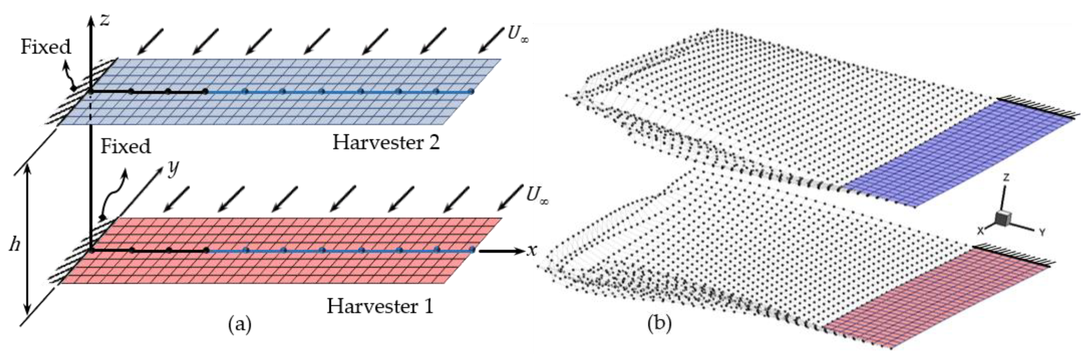
3.2. Case Study: Two Aerodynamically Coupled Harvesters

The case study considered herein consists of an array of two harvesters stacked vertically and separated by a vertical distance h (see Figure 11a). The main goal of this study is to characterize the combined piezoaeroelastic behavior of the system, quantifying the effect of the aerodynamic coupling between the harvesters. In order to assess the aerodynamic interaction, the flutter onset wind speed and the electrical output of the two-harvester system are compared with that of an isolated harvester. The model consists of two identical cantilevered harvesters, each with identical properties and discretization as the ones used in Section 3.1. Each harvester produces a vortex wake that is shed from the trailing edge and from the free tip of the plate, as shown schematically in Figure 11b.
For the first study on this configuration (Section 3.2.1), the influence of the separation distance h on the mutual interaction among harvesters and the global system characteristics are analyzed. For the last study (Section 3.2.2), the system’s postcritical behavior is studied for a particular fixed value of the separation h.

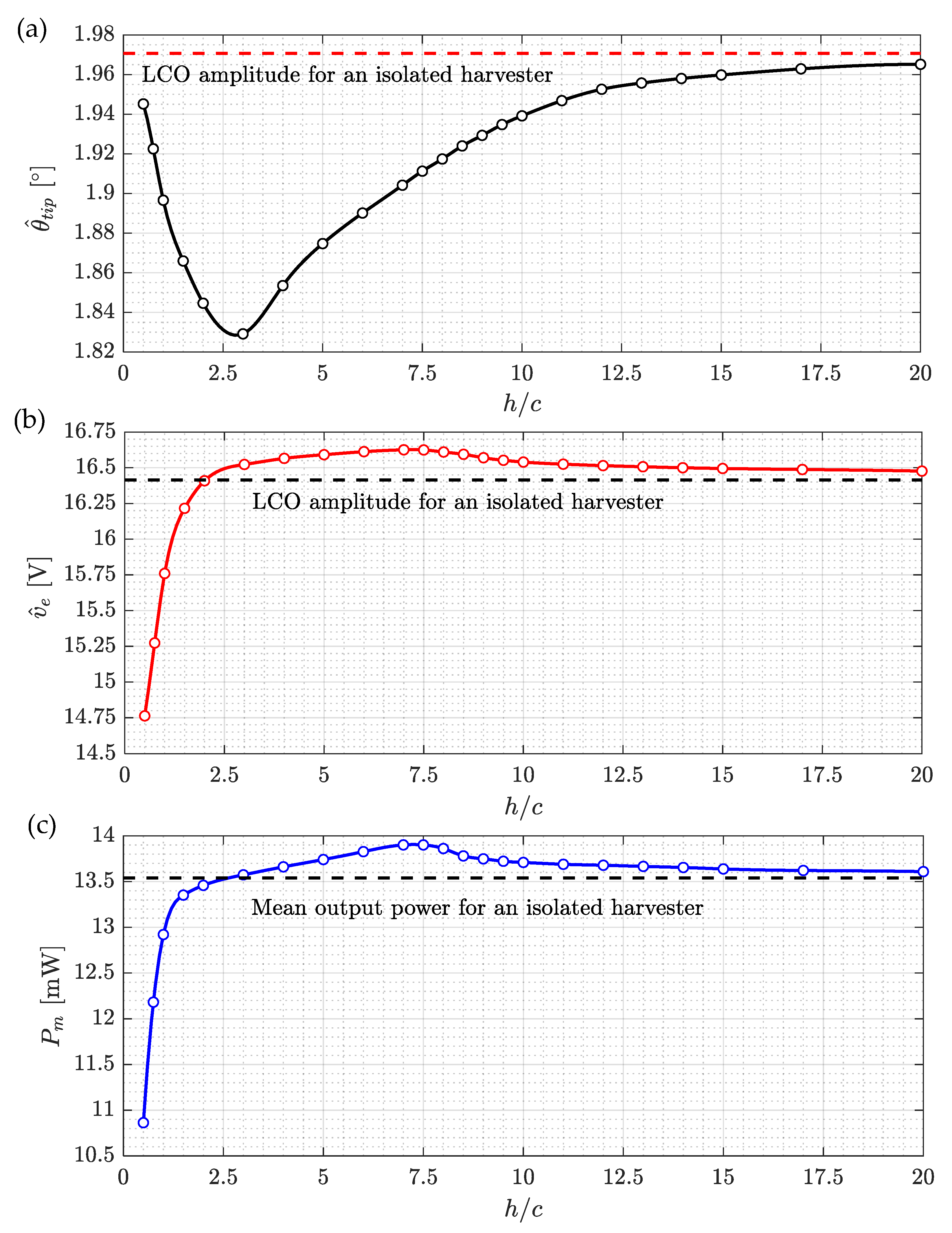
3.2.1. Influence of the Separation Distance

The flutter speed of the harvester array V F A was computed for increasing values of the separation distance h . The variation of the nondimensional flutter speed V F A ¯ with the vertical distance between the harvesters is shown in Figure 12 Here, V F A ¯ = V F A / V F I is the normalized flutter speed of the array with respect to the flutter speed V F I = 41.505 m/s of an isolated harvester.
Based only on the dependence of the flutter speed with the spacing h, two zones, favorable and unfavorable, are identified in Figure 12. It is recalled that each individual harvester in the system only undergoes self-sustaining limit cycle oscillations at or above the flutter speed. Therefore, a favorable characterization is given to the region where lower wind speeds are needed to achieve flutter. A lower flutter critical speed of the system allows the harvesters to operate over a wider range of free-stream wind velocities and to exploit the flutter phenomena at lower wind speeds, something otherwise impossible for the single isolated harvester configuration. Therefore, this scenario is deemed advantageous.
As it is shown in Figure 12, the transition between the favorable and unfavorable interaction zones occurs at a value of spacing h / c approximately equal to five. In the favorable zone, the flutter speed of the array is below the flutter speed of an isolated harvester ( V F A ¯ < 1 ). Conversely, in the unfavourable zone, the flutter speed of the array is above the flutter speed of an isolated harvester ( V F A ¯ < 1 ). In this last zone, it is observed that a maximum value of V ¯ F A is reached approximately at h / c = 7.5 . From this value on, on V F A decreases asymptotically approaching the reference value ( V F A ¯ = 1 ). This implies that as the distance increases beyond a certain point, the mutual aerodynamic interaction between harvesters becomes insignificant, and each harvester behaves effectively as if it was isolated.
Continuing with the analysis, the amplitudes of the LCO of the wing tip pitch angle θ ^ t i p and the output voltage v ^ e obtained at the flutter speed V F A of the array for different values of the gap h / c are presented in Figure 13. The value of the mean output electric power P m under the same conditions is shown Figure 13. These results correspond only to one of the harvesters in the array; thus, the total output power of the system is twice the value presented in Figure 13.
The amplitude of the LCO for the wing tip pitch angle is found to be smaller than the reference value corresponding to an isolated harvester across all the separation range considered. For values of h / c 3 , the amplitude θ ^ t i p is observed to decrease with increasing separation until a minimum value at approximately h / c = 3 is reached. From this value on, the amplitude of the pitching motion increases and slowly approaches the reference line.
The values of the amplitude of the output voltage v ^ e (Figure 13b) are well below the baseline value for small values of h / c . For h / c < 2.0 , the amplitude of the voltage LCO depicts a steep increase with the separation between harvesters. Approximately for h / c = 2 , the v ^ e curve crosses the reference value for an isolated harvester. Beyond this point, the voltage amplitude continues to increase until a maximum value is reached at h / c = 7.5 . For h / c > 7.5 the amplitude v ^ e decreases to asymptotically approach the baseline value.
The mean output power (Figure 13c) behaves qualitatively similar to the output voltage LCO amplitude. For values h / c < 3 , the presence of the second harvester produces the undesirable outcome of reducing the power harvested by each individual harvester. Approximately for h / c = 3 the mean power P m of each individual harvester in the system is the same as the mean power produced by an isolated harvester. For larger values of h / c , the power continues to grow to reach a maximum at h / c = 7.5 and finally decreases approaching the reference line.
Here, a holistic consideration is elaborated based on the results presented in Figure 12. It is observed that, for separation values h / c < 3 , the power output of each individual harvester is below their isolated values. This may suggest that the configuration is detrimental for the energy harvesting performance of each individual harvester. However, such values of the separation h / c lie within what was previously defined as the favorable zone. This means that each harvester is actually undergoing self-sustained LCO (flutter) and generating electrical power at values of the wind speed that would have resulted in no power output at all for a single isolated harvester. Hence, to be fair, a comparison should be made between the zero-power output of a single isolated harvester and the nonzero power output for the array of two harvesters at the given speed. From the above discussion, it is concluded that the definition of the favorable zone answers to the priority given to the ability to harvest energy at lower wind speeds. As a particular example, consider the case of two harvesters separated h / c = 0.5 where the mean power output of each harvester is about 20% lower than the value for an isolated harvester. For the same configuration, the system flutter speed is reduced by 22% with respect to the value for an isolated harvester. Therefore, the array is able to extract energy from a freestream with a 20% smaller speed when the isolated harvester would just simply stay still (or its oscillations damped out). Finally, it is recalled that although the power collected by each individual harvester is 20% lower, the combined power extracted by the two-harvester is actually 60% larger than that for a single isolated harvester. This means more power extraction at lower wind speeds but at a lower harvester individual efficiency.

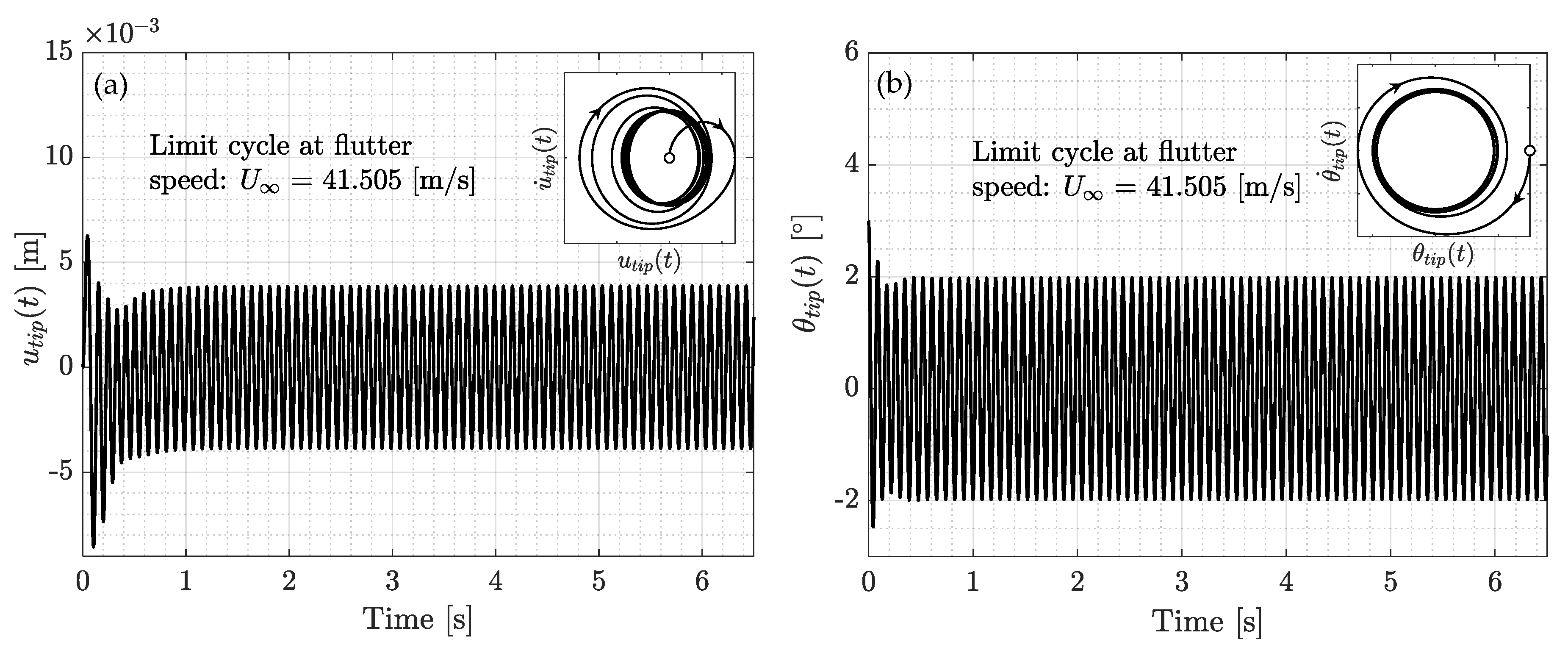
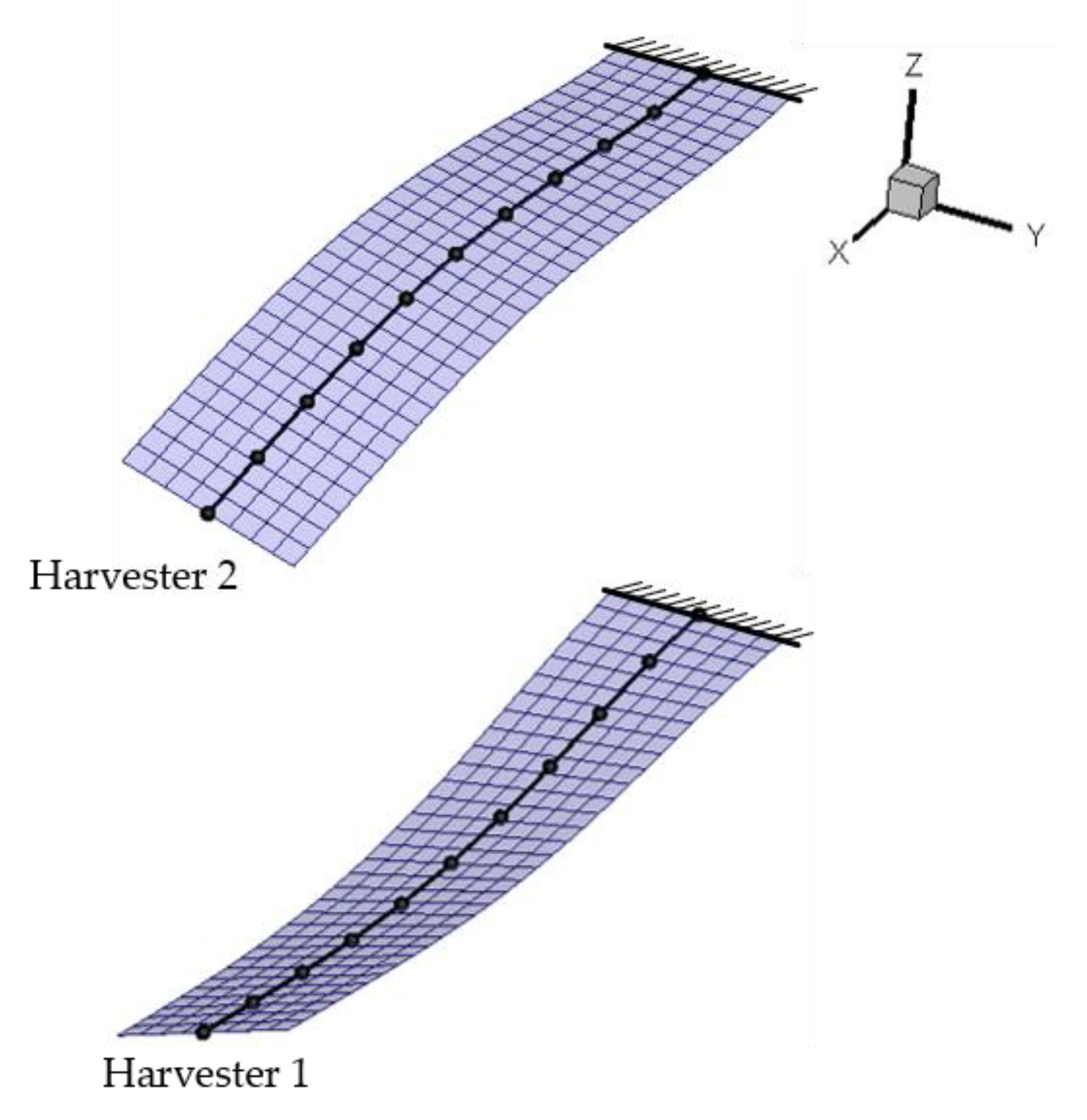
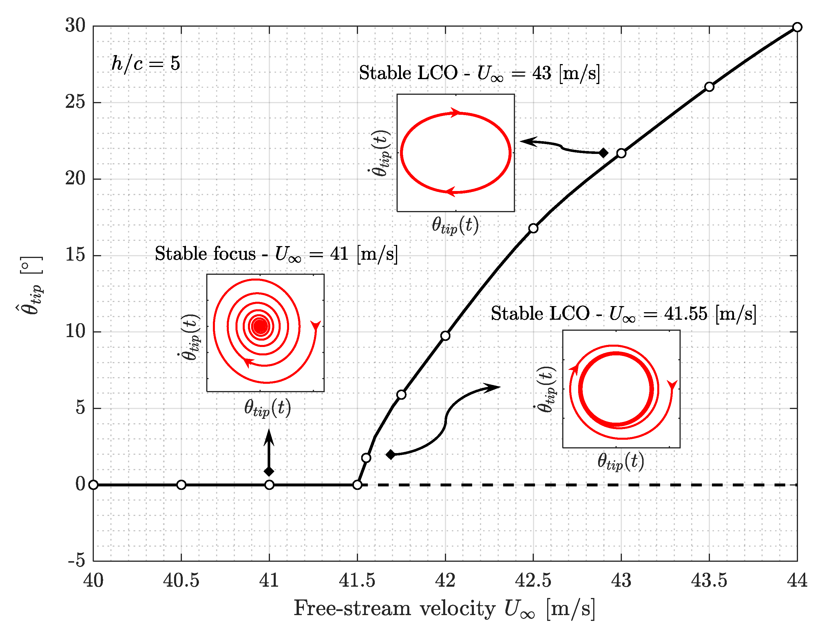
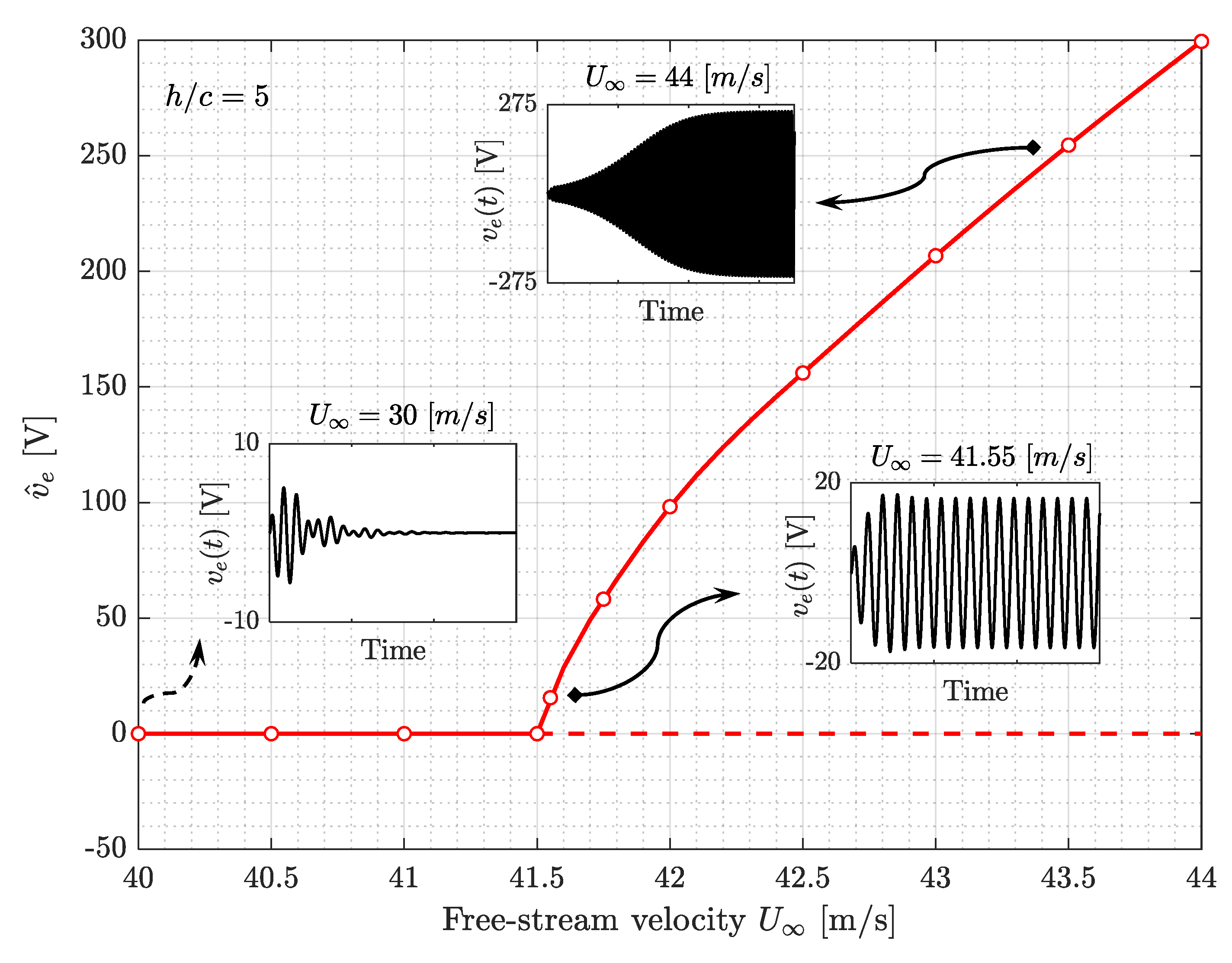
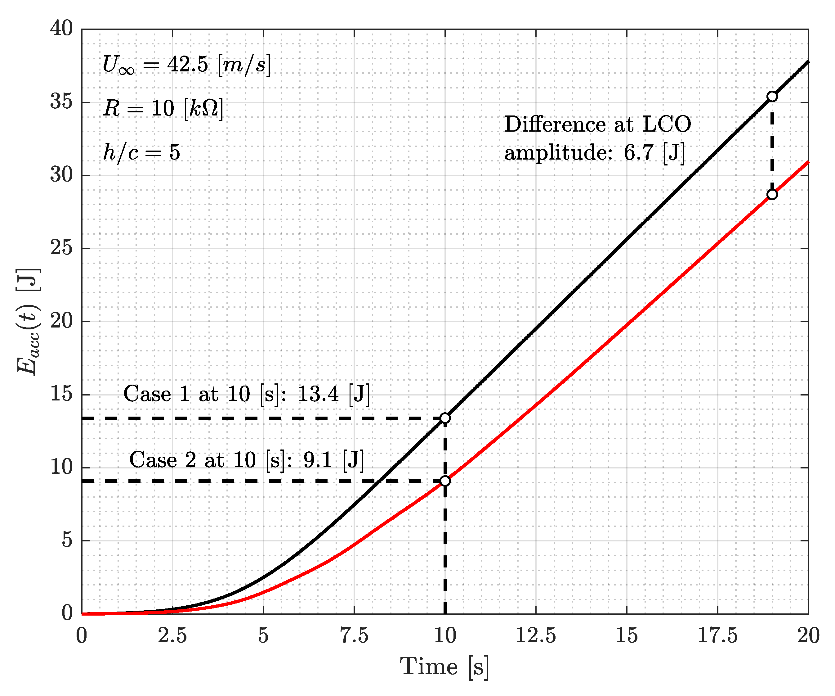
3.2.2. Postcritical Response Analysis

The postcritical behavior of the two-harvester array is analyzed for a fixed value of the dimensionless distance h / c = 5 . This separation is chosen because the flutter speed of the system was observed to be approximately equal to the value for an isolated harvester, whereas the voltage and power output are slightly higher due to the mutual aerodynamic interaction. For this particular case, the flutter mode shape, the postflutter behavior, and an analysis of the influence of initial conditions are presented.
As already mentioned, the flutter speed of the two-harvester system with h / c = 5 is equal to the value for one harvester; that is to say, V F A = 41.505 m/s. At this wind speed, because the frequencies of all the modes of the system coalesce into a unique value, the system response can be characterized through what is referred to as the flutter mode shape. This mode shape is presented in Figure 14. It can be observed that the mode consists of coupled bending–torsion motions and that the harvesters are in antiphase (with π radians phase offset), that is to say, the flutter mode is symmetric about the imaginary plane in-between the harvesters.
According to the model formulation, the weak aerodynamic interaction between the harvesters contributes sufficient enough nonlinearity to the system to allow postflutter bounded LCO. This is contrary to linear formulations that cannot predict the behavior past the critical speed. For the case under analysis, it is observed that once the flutter speed is exceeded, the system exhibits postcritical limit cycle oscillations. To provide an overall picture of the system response, the bifurcation diagram for the amplitude of the free tip pitch angle is presented in Figure 15. The presence of a supercritical Hopf bifurcation when the wind speed reaches the flutter critical speed is observed in this figure. For wind speeds below the critical speed, the phase diagram of θ t i p resembles the characteristic response of around a stable focus. In addition, it can be observed that the amplitudes of the LCOs monotonically increase for the range of velocities considered.
In Figure 16, a similar bifurcation diagram is presented for the output voltage amplitude. In line with the results for the pitch angle amplitude, the oscillations of the voltage output die away with time when the free-stream speed is below the flutter speed. For wind speeds beyond the flutter speed the output voltage exhibits self-sustained limit cycle oscillations with amplitude monotonically increasing with increasing wind speed.
A final analysis is performed to understand the influence of the initial conditions on the system outputs. For this purpose, the accumulated system electric energy as a function of time t is defined as follows:
E a c c ( t ) : = 0 t P ( τ )   d τ
where P ( τ ) = v e 2 ( τ ) / R is the instantaneous combined electrical power of the two harvesters.
The temporal evolution of E a c c is computed for two cases with different set of initial conditions:
  • Case 1: A 3 deg rotation of the free tip is imposed to both harvesters in a symmetrical configuration.
  • Case 2: A 3 deg rotation of the free tip is imposed only to the bottom harvester (Harvester 1).
The accumulated energy in time predicted for both cases is shown in Figure 17. It is observed that after a time of approximately 10 s, the accumulated energy in Case 1 is about 47% higher than the corresponding value for Case 2. In addition, the difference between the accumulated energy in both cases grows to reach a constant value of 6.7 J once the LCO amplitude is reached. At this point the curves become parallel to each other.
The time histories of the output voltage of each harvester for Cases 1 and 2 are presented in Figure 18. It is observed that for Case 1, the voltage signals of the harvesters are identical (despite the antiphase initial condition) and that both reach the limit cycle (LC) attractor in about 9 s. On the other hand, for Case 2, where only one of the harvesters has initial conditions, it is observed that the LC attractor is reached at a later time compared to the previous case, about 19 s after the start of the motion. Moreover, before reaching the LC, the amplitude of the output voltage of the harvesters appears to be modulated by envelopes that are lagged by 90 deg. This behavior could be interpreted as an exchange of energy between the harvesters. The behavior and the longer time to reach the LC may explain why for Case 2 total energy harvested is smaller than for Case 1.
The observed phenomena provide evidence of the relative importance of the initial conditions on the system’s harvesting performance when reduced periods of time are considered.

4. Conclusions

This effort is motivated by the need to understand the combined piezoelectric and aeroelastic behavior of arrays of flutter-based energy harvesters. The proposed array configuration is a potential technological solution to overcome the issue of low power outputs of single flutter-based energy harvesting systems. Insights on the effects of the weak aerodynamic coupling between the harvesters as a function of the separation between them are crucial for advancing the field towards reliable, wide operating range and high-power output harvesting systems. The studies presented in this article emphasize the capability of the developed approach to predict the piezoaeroelastic nonlinear response of harvester arrays.
To carry out the present study, a multiphysics framework based on a co-simulation strategy was developed. The three physics involved, fluid dynamics, structural mechanics, and piezoelectricity were represented as two independent, yet interacting, models: a UVLM-based model and computational implementation were developed to compute the aerodynamic forces, and a three-dimensional, a nonhomogeneous piezoelectric/elastic finite-element beam model was introduced to determine the structural response due to the fluid loads. The finite-element beam formulation is based on a classical Euler–Bernoulli beam augmented by the so-called von Kármán nonlinearities. The models were strongly coupled at the computational implementation level through a co-simulation scheme. This approach consists of a bidirectional exchange of information between the physics within an iteration loop at each time step and ensures convergence to a desired precision.
The correct implementation of the computational framework was verified by reproducing a study previously reported by other researchers in the literature. This study consisted of a single flutter-based piezoelectric power-generating wing whose flutter speed and frequency were estimated. The predictions of the current method were shown to agree well with those reported in the literature, thus providing confidence for its use on more complex systems and configurations.
The core study of this effort is on an array of two vertically stacked harvesters. The idea behind this configuration is exploiting the constructive aerodynamic interaction and synergy between the harvesters to enhance the overall performance of the system when compared to the typical single harvester configuration. In this article, the authors focus only on the effect of the vertical separation between harvesters over the cut-in speed of the system (the critical flutter speed at which the system starts harvesting). Other aspects, namely, horizontal separation, number of harvesters, structural coupling between harvesters, end boundary conditions, and so on, will be explored in future works.
From the results obtained, it can be concluded that the cut-in speed of the system can be substantially reduced with respect to the single harvester configuration when the spacing between the vertically stacked harvesters is below a certain threshold. For the particular geometry of the harvesters under study, the separation threshold was found to be approximately five chords. In view of this phenomenon, a favorable interaction region was identified for separation values below this threshold value. An array working in the favorable zone can harvest energy from the wind at speeds that would not induce any postcritical LCO, hence no energy output, on a single harvester alone. In addition, the system can be designed so that the gap between the harvesters can be varied during operation to accommodate the actual wind conditions. Finally, it was also observed that beyond the separation threshold, the cut-in speed and also the power output of each harvester in the array become larger than that of a single harvester configuration. As the separation becomes very large, the aerodynamic coupling between the harvesters becomes very weak, and each device in the array behaves effectively as if they were in a single harvester configuration.
The postcritical behavior of the harvesters is characterized by a supercritical Hopf bifurcation. At postcritical wind speed regimes, the weakly nonlinear aerodynamic interaction between the harvesters was observed to lead to stable LCOs with amplitudes that increase with increasing wind speeds. For these postcritical scenarios, the flutter mode shape could be extracted from the structural response of the system. It was observed that the flutter mode for each of the harvesters is a combination of bending and torsion modes. Moreover, the flutter modes of both harvesters together conform to a symmetric configuration (antiphase).
Finally, the cumulative extracted energy of the system in time was analyzed for two different sets of initial conditions. The goal of this final study was to better understand the transient effects of the nonlinear interaction and the impact of the initial conditions. The results obtained suggest that the initial conditions do have an impact on the elapsed time between the start of the motion and the moment when the stable limit cycle attractor is reached. Based on the observed histories of the accumulated energy, it is concluded that properly set initial conditions may reduce the time needed for the array to reach the attractor for its intended normal operation condition. The closer these initial conditions are to the flutter mode shape, the fastest the LC attractor is reached.
The promising findings reported in this article will help in filling in an important gap regarding the exploitation of constructive aerodynamic interaction and synergies for flutter-based energy harvesting. The results of this effort may find applications in the design and integration of low-energy wind generation technologies into buildings, bridges, and built-in sensor networks in aircraft structures.

Author Contributions

Conceptualization, B.A.R., M.F.V., M.L.V. and S.P.; Formal analysis, M.E.P.S.; Investigation, S.P.; Methodology, E.B., B.A.R., M.F.V., M.L.V. and S.P.; Project administration, S.P.; Resources, S.P.; Software, E.B. and M.E.P.S.; Supervision, S.P.; Validation, E.B., M.E.P.S. and M.L.V.; Visualization, E.B.; Writing—original draft, B.A.R., M.F.V. and M.L.V.; Writing—review & editing, B.A.R., M.F.V. and S.P. All authors have read and agreed to the published version of the manuscript.

Funding

This research was supported by Consejo Nacional de Investigaciones Científicas y Técnicas (CONICET), by Agencia Nacional de Promoción Científica y Tecnológica (ANPCyT), grant PICT 2016 number 1290, by Secretaría de Ciencia y Técnica, Universidad Nacional de Córdoba (SeCyT-UNC), grant number 33620180100563CB, as well as by Consejo de Investigación, Universidad Nacional de Salta (CIUNSa), grant Proyecto Tipo C number 2658.

Acknowledgments

We would like to express our deepest and sincere gratitude to our mentor, teacher, and beloved friend, Dean T. Mook, who passed away on 19 June 2020, for his support, contributions to our education, friendship, and for giving all of us the golden opportunity to work in this wonderful topic. Mook made important contributions to the development of applied mechanics in our country through personal interactions with many Argentinean colleagues and students. We have been blessed to have had Mook in our lives; to work with and to learn from him, as well as to be able to pass his teachings on through our own research and mentorship of others. He will be missed more than words can express.

Conflicts of Interest

The authors declare no conflict of interest.

References

  1. Hodges, D.H.; Pierce, G.A. Introduction to Structural Dynamics and Aeroelasticity; Cambridge University Press: Cambridge, UK, 2011; ISBN 9780511997112. [Google Scholar]
  2. Rostami, A.B.; Armandei, M. Renewable energy harvesting by vortex-induced motions: Review and benchmarking of technologies. Renew. Sustain. Energy Rev. 2017, 70, 193–214. [Google Scholar] [CrossRef]
  3. Bryant, M.; Garcia, E. Development of an aeroelastic vibration power harvester. In Proceedings of the SPIE Smart Structures and Materials + Nondestructive Evaluation and Health Monitoring, San Diego, CA, USA, 8–12 March 2009; p. 728812. [Google Scholar] [CrossRef]
  4. Dias, J.A.C.; De Marqui, C.; Erturk, A. Three-degree-of-freedom hybrid piezoelectric-inductive aeroelastic energy harvester exploiting a control surface. AIAA J. 2014, 53, 394–404. [Google Scholar] [CrossRef] [Green Version]
  5. Doarée, O.; Michelin, S. Piezoelectric coupling in energy-harvesting fluttering flexible plates: Linear stability analysis and conversion efficiency. J. Fluids Struct. 2011, 27, 1357–1375. [Google Scholar] [CrossRef] [Green Version]
  6. Erturk, A.; Vieira, W.G.R.; De Marqui, C.; Inman, D.J. On the energy harvesting potential of piezoaeroelastic systems. Appl. Phys. Lett. 2010, 96. [Google Scholar] [CrossRef]
  7. Safaei, M.; Sodano, H.A.; Anton, S.R. A review of energy harvesting using piezoelectric materials: State-of-the-art a decade later (2008–2018). Smart Mater. Struct. 2019, 28. [Google Scholar] [CrossRef]
  8. Elahi, H.; Eugeni, M.; Gaudenzi, P. A review on mechanisms for piezoelectric-based energy harvesters. Energies 2018, 11, 1850. [Google Scholar] [CrossRef] [Green Version]
  9. Yang, Z.; Zhou, S.; Zu, J.; Inman, D. High-performance piezoelectric energy harvesters and their applications. Joule 2018, 2, 642–697. [Google Scholar] [CrossRef] [Green Version]
  10. Bae, J.-S.; Inman, D.J. Aeroelastic characteristics of linear and nonlinear piezo-aeroelastic energy harvester. J. Intell. Mater. Syst. Struct. 2013, 25, 401–416. [Google Scholar] [CrossRef]
  11. Wu, Y.; Li, D.; Xiang, J.; Da Ronch, A. Piezoaeroelastic energy harvesting based on an airfoil with double plunge degrees of freedom: Modeling and numerical analysis. J. Fluids Struct. 2017, 74, 111–129. [Google Scholar] [CrossRef]
  12. Abdelkefi, A.; Nayfeh, A.H.; Hajj, M.R. Modeling and analysis of piezoaeroelastic energy harvesters. Nonlinear Dyn. 2012, 67, 925–939. [Google Scholar] [CrossRef]
  13. Abdelkefi, A.; Ghommem, M.; Nuhait, A.O.; Hajj, M.R. Nonlinear analysis and enhancement of wing-based piezoaeroelastic energy harvesters. J. Sound Vib. 2014, 333, 166–177. [Google Scholar] [CrossRef]
  14. Sousa, V.C.; de M Anicézio, M.; De Marqui, C., Jr.; Erturk, A. Enhanced aeroelastic energy harvesting by exploiting combined nonlinearities: Theory and experiment. Smart Mater. Struct. 2011, 20, 094007. [Google Scholar] [CrossRef]
  15. Zhao, Y.H.; Hu, H.Y. Aeroelastic analysis of a non-linear airfoil based on unsteady vortex lattice model. J. Sound Vib. 2004, 276, 491–510. [Google Scholar] [CrossRef]
  16. Dos Santos, C.R.; Marques, F.D.; Hajj, M.R. The effects of structural and aerodynamic nonlinearities on the energy harvesting from airfoil stall-induced oscillations. JVC J. Vib. Control 2019, 25, 1991–2007. [Google Scholar] [CrossRef]
  17. Bao, C.; Dai, Y.; Wang, P.; Tang, G. A piezoelectric energy harvesting scheme based on stall flutter of airfoil section. Eur. J. Mech. B Fluids 2019, 75, 119–132. [Google Scholar] [CrossRef]
  18. Abdelkefi, A.; Hajj, M.R.; Nayfeh, A.H. Sensitivity analysis of piezoaeroelastic energy harvesters. J. Intell. Mater. Syst. Struct. 2012, 23, 1523–1531. [Google Scholar] [CrossRef]
  19. Bryant, M.; Fang, A.; Garcia, E. Self-powered smart blade: Helicopter blade energy harvesting. In Proceedings of the SPIE Smart Structures and Materials + Nondestructive Evaluation and Health Monitoring, San Diego, CA, USA, 7–11 March 2010; p. 764317. [Google Scholar] [CrossRef]
  20. Elahi, H.; Eugeni, M.; Gaudenzi, P. Design and performance evaluation of a piezoelectric aeroelastic energy harvester based on the limit cycle oscillation phenomenon. Acta Astronaut. 2019, 157, 233–240. [Google Scholar] [CrossRef]
  21. Eugeni, M.; Elahi, H.; Fune, F.; Lampani, L.; Mastroddi, F.; Romano, G.P.; Gaudenzi, P. Numerical and experimental investigation of piezoelectric energy harvester based on flag-flutter. Aerosp. Sci. Technol. 2020, 97, 105634. [Google Scholar] [CrossRef]
  22. Elahi, H.; Eugeni, M.; Fune, F.; Lampani, L.; Mastroddi, F.; Romano, G.P.; Gaudenzi, P. Performance evaluation of a piezoelectric energy harvester based on flag-flutter. Micromachines 2020, 11, 933. [Google Scholar] [CrossRef]
  23. Zhu, D.; Tudor, M.J.; Beeby, S.P. Strategies for increasing the operating frequency range of vibration energy harvesters: A review. Meas. Sci. Technol. 2010, 21. [Google Scholar] [CrossRef]
  24. Zhu, D.; Beeby, S.; Tudor, J.; White, N.; Harris, N. A novel miniature wind generator for wireless sensing applications. In Proceedings of the IEEE Sensors, Kona, HI, USA, 1–4 November 2010; pp. 1415–1418. [Google Scholar]
  25. Hu, G.; Wang, J.; Su, Z.; Li, G.; Peng, H.; Kwok, K.C.S. Performance evaluation of twin piezoelectric wind energy harvesters under mutual interference. Appl. Phys. Lett. 2019, 115, 1–5. [Google Scholar] [CrossRef]
  26. Abdelkefi, A.; Scanlon, J.M.; McDowell, E.; Hajj, M.R. Performance enhancement of piezoelectric energy harvesters from wake galloping. Appl. Phys. Lett. 2013, 103, 033903. [Google Scholar] [CrossRef] [Green Version]
  27. Zhao, L.; Yang, Y. An impact-based broadband aeroelastic energy harvester for concurrent wind and base vibration energy harvesting. Appl. Energy 2018, 212, 233–243. [Google Scholar] [CrossRef]
  28. Bibo, A.; Abdelkefi, A.; Daqaq, M.F. Modeling and characterization of a piezoelectric energy harvester under combined aerodynamic and base excitations. J. Vib. Acoust. Trans. ASME 2015, 137. [Google Scholar] [CrossRef]
  29. Hafezi, M.; Mirdamadi, H.R. A novel design for an adaptive aeroelastic energy harvesting system: Flutter and power analysis. J. Braz. Soc. Mech. Sci. Eng. 2019, 41. [Google Scholar] [CrossRef]
  30. Bryant, M.; Mahtani, R.L.; Garcia, E. Wake synergies enhance performance in aeroelastic vibration energy harvesting. J. Intell. Mater. Syst. Struct. 2012, 23, 1131–1141. [Google Scholar] [CrossRef]
  31. McCarthy, J.M.; Deivasigamani, A.; Watkins, S.; John, S.J.; Coman, F.; Petersen, P. On the visualisation of flow structures downstream of fluttering piezoelectric energy harvesters in a tandem configuration. Exp. Therm. Fluid Sci. 2014, 57, 407–419. [Google Scholar] [CrossRef]
  32. Deivasigamani, A.; Mccarthy, J.; John, S.; Watkins, S.; Coman, F. Proximity effects of piezoelectric energy harvesters in fluid flow. In Proceedings of the 29th Congress of the International Council of the Aeronautical Science, St. Petersburg, Russia, 7–12 September 2014. [Google Scholar]
  33. Roccia, B.A.; Verstraete, M.L.; Ceballos, L.R.; Balachandran, B.; Preidikman, S. Computational study on aerodynamically coupled piezoelectric harvesters. J. Intell. Mater. Syst. Struct. 2020, 31, 1578–1593. [Google Scholar] [CrossRef]
  34. Kirschmeier, B.; Bryant, M. Experimental investigation of wake-induced aeroelastic limit cycle oscillations in tandem wings. J. Fluids Struct. 2018, 81, 309–324. [Google Scholar] [CrossRef]
  35. McCarthy, J.M.; Watkins, S.; Deivasigamani, A.; John, S.J. Fluttering energy harvesters in the wind: A review. J. Sound Vib. 2016, 361, 355–377. [Google Scholar] [CrossRef]
  36. Katz, J.; Plotkin, A. Low-speed aerodynamics, second edition. J. Fluids Eng. 2004, 126, 293–294. [Google Scholar] [CrossRef] [Green Version]
  37. Van Garrel, A. Development of a Wind Turbine Aerodynamics Simulation Module; Energy research Centre of the Netherlands ECN: Petten, The Netherlands, 2003. [Google Scholar]
  38. Chopra, I.; Sirohi, J. Smart Structures Theory; Cambridge University Press: Cambridge, UK, 2013; ISBN 9781139025164. [Google Scholar]
  39. Auricchio, F.; Carotenuto, P.; Reali, A. On the geometrically exact beam model: A consistent, effective and simple derivation from three-dimensional finite-elasticity. Int. J. Solids Struct. 2008, 45, 4766–4781. [Google Scholar] [CrossRef] [Green Version]
  40. Hassanpour, S.; Heppler, G.R. Approximation of infinitesimal rotations in calculus of variations. J. Guid. Control. Dyn. 2016, 39, 703–710. [Google Scholar] [CrossRef]
  41. Andersen, L.; Nielsen, S.R.K. Elastic Beams in Three Dimensions; Department of Civil Engineering, Aalborg University: Aalborg, Denmark, 2008. [Google Scholar]
  42. Reddy, J.N. An Introduction to Nonlinear Finite Element Analysis, 2nd ed.; Oxford University Press: Oxford, UK, 2010; ISBN 978-0199641758. [Google Scholar]
  43. Lerch, R. Simulation of piezoelectric devices by two- and three-dimensional finite elements. IEEE Trans. Ultrason. Ferroelectr. Freq. Control 1990, 37, 233–247. [Google Scholar] [CrossRef]
  44. Allik, H.; Hughes, T.J.R. Finite element method for piezoelectric vibration. Int. J. Numer. Methods Eng. 1970, 2, 151–157. [Google Scholar] [CrossRef]
  45. Brannon, R. Rotation Reflection and Frame Changes Orthogonal Tensors in Computational Engineering Mechanics; IOP Publishing: Bristol, UK, 2018. [Google Scholar]
  46. Przemieniecki, J.S. Theory of Matrix Structural Analysis; Courier Corporation: North Chelmsford, Chelmsford, MA, USA, 1985; ISBN 0486649482. [Google Scholar]
  47. Beltramo, E.; Balachandran, B.; Preidikman, S. Three-dimensional formulation of a strain-based geometrically nonlinear piezoelectric beam for energy harvesting. J. Intell. Mater. Syst. Struct. 2020. submitted. [Google Scholar]
  48. Preidikman, S. Numerical Simulations of Interactions among Aerodynamics, Structural Dynamics, and Control Systems. Ph.D. Thesis, Department of Engineering Science and Mechanics, Virginia Polytechnic Inst. and State University, Blacksburg, VA, USA, 1998. [Google Scholar]
  49. Konstandinopoulos, P.; Mook, D.T.; Nayfeh, A. A Numerical Method for General, Unsteady Aerodynamics; American Institute of Aeronautics and Astronautics (AIAA): Reston, VA, USA, 1981. [Google Scholar]
  50. Roccia, B.A.; Preidikman, S.; Massa, J.C.; Mook, D.T. Modified unsteady vortex-lattice method to study flapping wings in hover flight. AIAA J. 2013, 51, 2628–2642. [Google Scholar] [CrossRef] [Green Version]
  51. Carnahan, B.; Luther, H.A. Applied Numerical Methods; Wiley: New York, NY, USA, 1969. [Google Scholar] [CrossRef]
  52. Roccia, B.A.; Preidikman, S.; Balachandran, B. Computational dynamics of flapping wings in hover flight: A co-simulation strategy. AIAA J. 2017, 55, 1806–1822. [Google Scholar] [CrossRef]
  53. De Marqui, C.; Erturk, A.; Inman, D.J. Piezoaeroelastic modeling and analysis of a generator wing with continuous and segmented electrodes. J. Intell. Mater. Syst. Struct. 2010, 21, 983–993. [Google Scholar] [CrossRef]
  54. De Marqui, C.; Vieira, W.G.R.; Erturk, A.; Inman, D.J. Modeling and analysis of piezoelectric energy harvesting from aeroelastic vibrations using the doublet-lattice method. J. Vib. Acoust. Trans. ASME 2011, 133. [Google Scholar] [CrossRef] [Green Version]
Figure 1. Schematic representation of the vortex lattice discretization of the bound vortex sheet on a solid surface. Finite-length vortex segments with circulations Δ Γ 1 j , k and Δ Γ 2 j , k are used to discretize the continuous vorticity distribution over the surface. The subindices 1 and 2 indicate two directions of discretization. When connected, these vortex segments form vortex rings whose circulation is conserved spatially.
Aerospace 07 00167 g001
Figure 2. Velocity V L ( r ) at location r due to an oriented vortex segment of length L and constant circulation Δ Γ .
Aerospace 07 00167 g002
Figure 3. Schematic representation of the flow separation from the trailing edge at t = Δ t . This process is repeated every time step, whereas the previously created wake vortex rings are convected with the local fluid velocity according to Equation (14).
Aerospace 07 00167 g003
Figure 4. (a) Schematic representation of the layered piezoelectric beam: (b) detail of the electric connection for the piezoelectric layers, and (c) lateral view of a generic piezoelectric layer.
Aerospace 07 00167 g004
Figure 5. Typical finite-element beam with six degrees of freedom per node.
Aerospace 07 00167 g005
Figure 6. Schematic diagram of the transfer technique between the structural and the aerodynamic models.
Aerospace 07 00167 g006
Figure 7. Reproduction of the physical model proposed in [53,54].
Aerospace 07 00167 g007
Figure 8. Numerical model of piezoelectric-based power-generating wing.
Aerospace 07 00167 g008
Figure 9. Simulation results wind speed equal to the flutter speed U = 41.50 m/s. (a) Time history and phase portrait for the wing tip vertical displacement u t i p ( t ) ; (b) time history and phase portrait for the wing tip rotation θ t i p ( t ) .
Aerospace 07 00167 g009
Figure 10. Fast Fourier Transform (FFT) at flutter speed U = 41.505 m/s for u t i p ( t ) and θ t i p ( t ) .
Aerospace 07 00167 g010
Figure 11. Schematic representation of an array of two harvesters. (a) Model setup; (b) wakes visualization.
Aerospace 07 00167 g011
Figure 12. Nondimensional flutter speed V F A ¯ as a function of the nondimensional separation distance h / c between harvesters.
Aerospace 07 00167 g012
Figure 13. Output variables obtained during limit cycle oscillations (LCO) at the flutter speed of a two-harvester array as a function of the nondimensional separation distance h / c . (a) Amplitude of the pitch angle at the tip θ ^ t i p ; (b) amplitude of the output voltage of one harvester v ^ e ; (c) mean electrical power output P m .
Aerospace 07 00167 g013
Figure 14. Flutter mode shape for an array of two vertically stacked harvesters with gap h / c = 5 .
Aerospace 07 00167 g014
Figure 15. Bifurcation diagram of the tip pitch angle θ ^ t i p of one of the harvesters in a two-harvester array with separation h / c = 5 .
Aerospace 07 00167 g015
Figure 16. Bifurcation diagram for the output voltage v ^ e of one of the harvesters in a two-harvester array with separation h / c = 5 .
Aerospace 07 00167 g016
Figure 17. Temporal evolution of the accumulated electric energy E a c c of a two-harvester array with separation h / c = 5 obtained for two different sets of initial conditions.
Aerospace 07 00167 g017
Figure 18. Output voltage of each individual harvester in a two-harvester array with separation h / c = 5 obtained for two different sets of initial conditions.
Aerospace 07 00167 g018
Table 1. Geometrical and mechanical properties of the physical model of De Marqui et al. [53,54].
PropertyValue
Piezoceramic transducers
MaterialPZT-5A
Length ( l 1 ) [mm]400
Thickness ( t 1 ) [mm]0.5
Width ( b ) [mm]240
Electrical resistance ( R ) [kΩ]10
Substrate
Young’s modulus [Gpa]70
Constant ( α ) [rad/s]0.1635
Constant ( β ) [s/rad]4.1711 × 10−4
Mass density [kg/m3]2750
Length ( l 2 ) [mm]800
Thickness ( t 2 ) [mm]2
Thickness ( t 3 ) [mm]3
Airflow
Air density [kg/m3]1.225
Reynolds Number
Table 2. Comparison of results between the present model and the model of De Marqui et al.
CharacteristicPresent ModelDe Marqui et al.Error
f 1 (Bending) [Hz]1.63361.682.76%
f 2 (Bending) [Hz]10.205010.462.48%
f 3 (Torsion) [Hz]16.846316.661.11%
f 4 (Bending) [Hz]27.015527.742.61%
f 5 (Torsion) [Hz]48.071148.651.20%
Flutter Frequency f f [Hz]11.5511.470.70%
Flutter Speed [m/s]41.0540.51.35%
Publisher’s Note: MDPI stays neutral with regard to jurisdictional claims in published maps and institutional affiliations.

