How Well Can Persistent Contrails Be Predicted?


1
Deutsches Zentrum für Luft- und Raumfahrt, Institut für Physik der Atmosphäre, D-82234 Oberpfaffenhofen, Germany
2
Forschungszentrum Jülich, IEK-8, D-52425 Jülich, Germany
*
Author to whom correspondence should be addressed.
Aerospace 2020, 7(12), 169; https://doi.org/10.3390/aerospace7120169
Submission received: 29 October 2020
/
Revised: 20 November 2020
/
Accepted: 27 November 2020
/
Published: 2 December 2020
(This article belongs to the Special Issue Selected Papers from 3rd ECATS Conference on Making Aviation Environmentally Sustainable)
Abstract
:Persistent contrails and contrail cirrus are responsible for a large part of aviation induced radiative forcing. A considerable fraction of their warming effect could be eliminated by diverting only a quite small fraction of flight paths, namely those that produce the highest individual radiative forcing (iRF). In order to make this a viable mitigation strategy it is necessary that aviation weather forecast is able to predict (i) when and where contrails are formed, (ii) which of these are persistent, and (iii) how large the iRF of those contrails would be. Here we study several data bases together with weather data in order to see whether such a forecast would currently be possible. It turns out that the formation of contrails can be predicted with some success, but there are problems to predict contrail persistence. The underlying reason for this is that while the temperature field is quite good in weather prediction and climate simulations with specified dynamics, this is not so for the relative humidity in general and for ice supersaturation in particular. However we find that the weather model shows the dynamical peculiarities that are expected for ice supersaturated regions where strong contrails are indeed found in satellite data. This justifies some hope that the prediction of strong contrails may be possible via general regression involving the dynamical state of the ambient atmosphere.
1. Introduction
Persistent contrails contribute substantially to the climate effect of aviation (for recent estimates see, e.g., [1,2,3]). Before the shutdown of aviation early this year as a consequence of the COVID-19 pandemic, aviation demand continued its steady increase and the annual total fuel consumption and emission of carbon dioxide increased at an annual rate of % per year in the period from 2010 to 2018, in spite of growing engine efficiency and load factors [3]. The growth rates are higher in non-OECD than in OECD countries which implies that contrail coverage might grow especially in regions where they were rare in the past. The annual and global mean radiative forcing (RF) of all contrails is of the order 50 mW/m, which represents a third to one half of the total estimated RF of aviation. The instantaneous RF of a single contrail (iRF) can, however, be three orders of magnitude larger with both negative (cooling) and positive (warming) sign, such that the value reported by the Intergovernmental Panel on Climate Change (IPCC) and in the estimates mentioned above is just the small net effect that remains when large negative and positive contributions almost balance. The balance is not perfect, such that a small positive RF remains.
There are two atmospheric conditions necessary for persistent contrails. First, the so called Schmidt-Appleman [4] criterion must be fulfilled, which is a pure thermodynamic criterion that rules whether contrail formation is possible in a given situation or not. This criterion covers both short-term (lifetime seconds to a few minutes) and persistent contrails. Thus a second condition is required for persistent contrails: the ambient air must be in a state of ice supersaturation, that is, the relative humidity with respect to ice, must exceed 100% [5]. Only then, the ice crystals the contrail consists of, can grow or at least they do not sublimate as long as %. Measurement of Ozone and Water Vapour on Airbus In-service Aircraft [MOZAIC [6]] data show that averaged over all flights, an aircraft is in about 15% of its cruise distances in ice supersaturated regions [ISSRs [7]], and persistent contrails could in principle be avoided if aircraft would not fly in ISSRs [8]. However, newer results obtained from the MOZAIC data [9,10] demonstrate that the mentioned average value of 15% is an average of very few ISSRs above the tropopause (around %) and around 30% below it in the uppermost troposphere. That is, there is almost no need for aviation to consider ice supersaturation in the lowermost stratosphere, where about 40% of cruise distances are flown [11], but it is considerably more difficult to avoid flying in ISSRs at cruise levels below the tropopause, in particular when these occur in regions with high air traffic density. Furthermore avoiding ISSRs generally involves deviations from a straight flight path which leads to higher costs, longer flight time, more fuel consumption and higher amounts of other emissions that are bad for climate (e.g., CO, NO, etc.).
To mitigate contrail induced warming of the climate, it is not efficient to avoid all persistent contrails. Avoiding only those ones that produce individually the largest warming [measured for instance in terms of energy forcing, EF, see [12,13]] suffices to largely eliminate the overall climate effect of persistent contrails. For instance, demonstrated in a study using data from six weeks of airtraffic in Eastern Asia that only about 2% of all flight distances contribute 80% to the total EF of all flights together [14]. These especially strong contrails are called Big Hits [15]. Ref. [14] show that selectively diverting % of the considered flights could lead to almost 60% reduction of contrail EF, and the corresponding increase in fuel consumption and CO emission would be % for the considered fleet. The authors considered a low-risk strategy as well, where flights are only diverted if there is no need for additional fuel; in this case the total EF could still be reduced by 20%.
This indicates that a large fraction of contrail induced aviation climate warming could be avoided at relatively low cost for additional fuel and at relatively little additional emissions of other greenhouse gases, if we knew in advance, where and when an aircraft will produce not only a contrail, but a persistent one with large individual instantaneous radiative forcing (iRF), and perhaps with long life-time and large horizontal spreading (since the EF is a time integral over contrail life-time of iRF within the time-dependent contrail area, length × width). Thus we need the capability to predict Big Hits, which is a challenge because, as mentioned, we are looking for those few percent of flight distances that are prone to produce Big Hit contrails.
In the present paper we concentrate on contrail persistence and on the instantaneous radiative forcing, that is the difference in the net (longwave plus shortwave) radiative flux at the top of the atmosphere between a situation with and an otherwise identical situation without a contrail. As a weather forecast we use reanalysis data of the European Centre for Medium-Range Weather Forecast (ECMWF), more precisely its reanalysis 5 (ERA-5) [16], and compare its "predictions" with data measured from satellites and commercial aircraft. We use these data to compute whether (i) contrail formation is possible at all (Schmidt-Appleman criterion), (ii) whether a contrail would be persistent (ice-supersaturation, ISSR), and (iii) finally if (i) and (ii) are true, we compute iRF from the reanalysis data and compare it to corresponding satellite-derived data.
2. Data and Methods
2.1. Data from Commercial Aircraft
The Measurement of Ozone and Water Vapour on Airbus In-service Aircraft (MOZAIC) programme [6] started in August 1994 and was transferred into the new European Research Infrastructure IAGOS (In-service Aircraft for a Global Observing System, www.iagos.org) [17] in 2011. It is an observing system installed on a small number of commercial passenger aircraft; it started with measurements of ozone and water vapour (relative humidity), but now it measures other species as well (CO, nitrogen containing species, aerosol and cloud particles). Until today (March 2020) more than 60,000 flights contributed to the data base. Here we use only temperature and relative humidity. Flight position (longitude, latitude, pressure altitude) are given for each data record. The data contain also quality labels for each record. We use only data with quality flag “0”, which means that the measurement is reliable. Records with (or %, i.e., water supersaturation) are rejected.
For the current study we select months of data that represent the four seasons: January, April, July and October 2014. For these months we have simulation results available obtained using the Earth System model EMAC [18], see below. 230 flights from Europe to mainly Asia and North-America have been selected from the data base. Only cruise level data have been retained with pressure altitudes between 310 hPa and 190 hPa.
The routes covered in these data are mostly between Europe (Frankfurt, Germany) and either North America (Montreal, Canada, and destinations from the eastcoast to the westcoast in the United States), Africa (Khartoum and Addis Abeba), and Asia (mainly destinations in Japan, China and India, but also Dubai and Tehran).
MOZAIC data are recorded every 4 seconds. In order to avoid autocorrelation we select about 1% of all data points by invoking a (0,1)-uniform random number generator. We proceed with the analysis of an individual record only when the random variate is smaller than . This procedure secures the mutual independence of single data points. For each selected data point we then collect the corresponding data (humidity, temperature, ice cloud water content, radiation quantities) from ERA-5, see below.
2.2. Satellite Data
The Automatic Contrail Tracking Algorithm (ACTA) [19] is a tool to spot and track individual contrails during part of their life. It uses the Rapid Scan Service of the Meteosat Second Generation satellite to track contrails in 5 min intervals over the heavily flown areas of the North-Atlantic and Europe. The ACTA data set spans a full year and contains observational records of 2305 individual contrails, including their optical thickness, computed using the COCS algorithm [20], their effects on the radiation field at the top of the atmosphere, computed using the RRUMS algorithm [21], as well as their length and width. The data set is described in detail in [22].
The ACTA data set has been applied to determine the statistical distribution of contrail lifetimes [23], but here we will use it to study two cases where the RRUMS algorithm indicated very strong positive iRF. We selected two situations: (a) 25 August 2008, between 2235 and 2255 UTC at about 7 W, 41 N in about 12 km altitude, and (b) 15 May 2009, between 1740 and 1830 UTC at about 25 W, 33 N in about 12 km altitude, about 750 km west of Madeira. Both cases are night-time cases, such that the shortwave fluxes are zero. The iRF indicated in the data exceeds for both cases 50 W m. The optical thickness of these contrails (or more precisely, contrail segments) are to and to , respectively.
2.3. Reanalysis Data
ERA-5 data have been retrieved from the Copernicus Data Service [16]. We use dynamic and thermodynamic data on four pressure levels: 200, 225, 250 and 300 hPa, as well as radiation flux densities at the top of the atmosphere (i.e., the highest model level). Data are retrieved in two versions, one for the comparison with aircraft data, and another for a small selection of cases from satellite observations.
For comparison with aircraft data we use data from four months in 2014 selected above that each represents another season: January, April, July and October. The horizontal resolution is and data cover the northern hemisphere between the equator and N. Temporal resolution is one hour. We selected the pressure level fields cloud ice water content, relative humidity and temperature. Note that relative humidity is to be understood with respect to ice at temperatures lower than C in ERA-5. Additionally we use the radiation quantities mean top downward shortwave radiation flux, mean top net longwave radiation flux, and mean top net shortwave radiation flux. In ERA-5 these quantities are flux densities in W/m averaged over the hour preceeding the respective valid (output) time.
For the analysis of the two ACTA cases we retrieved reanalysis data from ERA-5 for two longitude-latitude areas, with a spatial resolution of , and for each 6 hours before and around the event with hourly resolution. Pressure levels are as above. For these case studies we retrieved dynamical quantities as well, that is, geopotential, divergence, vorticity, three velocity components (), and potential vorticity.
2.4. EMAC Simulation Data
For further comparison we use results from the ECHAM/MESSy Atmospheric Chemistry (EMAC) model which is a numerical chemistry and climate simulation system that includes sub-models describing tropospheric and middle atmosphere processes and their interaction with oceans, land and human influences [24]. It uses the second version of the Modular Earth Submodel System (MESSy2) to link multi-institutional computer codes. The core atmospheric model is the 5th generation European Centre Hamburg general circulation model (ECHAM5) [25]. For the present study we applied EMAC (ECHAM5 version 5.3.02, MESSy version 2.54.0) in the T42L90MA-resolution, i.e., with a spherical truncation of T42 (corresponding to a quadratic Gaussian grid of approx. 2.8 by 2.8 degrees in latitude and longitude) with 90 vertical hybrid pressure levels up to 0.01 hPa. We perform a hindcast simulation with specified dynamics, i.e., ERA-Interim reanalysis data serve as time dependent boundary conditions for the model in order to perform a simulation with specified dynamics for the year 2014 [18]. For the retrieval of atmospheric parameters along the aircraft trajectories of IAGOS aircraft we use a diagnostics module for online sampling, which extracts the value of temperature, relative humidity, etc., in the grid cell at the respective geographic position and altitude with a temporal resolution of 12 min.
2.5. Methods
For the comparison of ERA-5 with the selected MOZAIC data we use the actual time and position of the aircraft, including its flight pressure level, and determine the corresponding atmospheric properties by quadrilinear interpolation in the meteorological data set. If the actual aircraft flight level is between 310 and 300 hPa, or between 200 and 190 hPa, interpolation in the vertical direction is not performed. Instead the values at 300 or 200 hPa are used.
For EMAC we use 660 points along various MOZAIC flights in the first half of April 2014. These points are all between 190 and 310 hPa, as before. They are each 12 min apart (time step of the model) which translates to about 150 km flight distance. For the comparison we match the coordinates and times with the closest MOZAIC measurement. We didn’t use 12-min averages since contrail formation is a local phenomenon, not an average one.
For the comparison with the ACTA data we use more (6) time points than actually necessary (2). The idea behind this is to not only perform the best matching but to look as well at the development of the synoptic situation over six hours.
For the calculation of iRF we use radiation formulae from [26] with constants for “Myhre particles”. These are pseudo-particles with wavelenght-independent optical properties. We consider this simplification sufficient for the present purpose. The required radiation quantities are included in the ERA-5 data. We identify outgoing longwave radiation (OLR) flux with mean top net longwave radiation flux, solar direct radiation (SDR) with mean top downward shortwave radiation flux, and reflected solar radiation (RSR) flux with mean top net shortwave radiation flux. The effective albedo is RSR/SDR during sunlit hours and zero at night. The solar constant is set to 1361 W m. To compute optical thickness of contrails and nearby cirrus we use a simple formulation [27]. The necessary vertical extensions are assumed as 500 m for contrails and 1500 m for cirrus. Effective radii of ice crystals are taken as m for contrails and m for cirrus. Furthermore we need the ice concentration, for which we assume that all water mass in excess of ice saturation is condensed as ice. The iRF is computed for all grid and time points that correspond to a selected MOZAIC data record (if a persistent contrail is possible). The calculation is done using the relative humidity and temperature of both data sets, MOZAIC and ERA-5. Differences in iRF are thus due to differences in temperature and relative humidity alone.
The calculation of the Schmidt-Appleman criterion assumes an overall propulsion efficiency of .
3. Results
We begin with the statistical analysis using the comparison between MOZAIC and ERA-5 data to obtain general results. Then we proceed with the two ACTA cases.
3.1. Statistical Analysis
3.1.1. Conditions for Contrail Formation and Persistence
The condition for contrail formation is that the so called Schmidt-Appleman criterion [4] is fulfilled. In words, it says that the mixture consisting of the expanding exhaust gases and ambient air must transiently become water saturated during the expansion of the plume. This can be cast into the physical terms of the maximum temperature, , at which contrail formation is still possible and the relative humidity the mixture obtains at the moment when it has temperature . The Schmidt-Appleman criterion can then be expressed as follows: contrails form once the ambient temperature is below and (logical and) (100%). Note that can be negative for situations with . In this case it has no physical meaning. We prefer to express the contrail formation conditions in terms of because its value has implications for contrail microphysics as well: the fraction of exhaust soot particles that serve as condensation and ice forming nuclei increases with , that is, with the attained supersaturation with respect to liquid water.
Figure 1 shows from MOZAIC flights on the x-axis and from corresponding ERA-5 data on the y-axis. We use here a random selection of about 1% of all flight data in order to avoid autocorrelation (see Section 2.1). That is, the figure (and others to come) displays a sample. The data pairs follow the diagonal line (black) quite well in the four considered months (colour coded). A seasonal variation can be seen with the lowest values in summer and the highest in winter. The upper half of Table 1 casts the comparison between the two data sets into a contingency table with the following entries:
- Y/Y, hits: MOZAIC data show that a contrail is formed and the corresponding interpolated ERA-5 data have properties that would allow contrail formation as well.
- Y/N, miss: While the MOZAIC aircraft produces a contrail, ERA-5 data do not indicate that contrail formation is possible.
- N/Y, false alarm: While the MOZAIC aircraft does not produce a contrail, ERA-5 data indicate that contrails are possible.
- N/N, correct negatives: ERA-5 data indicate that contrail formation is impossible and indeed there was no contrail formed by the MOZAIC aircraft.
The interpretation of the contingency table is explained in Appendix A where we also introduce the equitable threat score, ETS, that we use to characterise the degree of agreement between the two data sets. Reasons for using ETS instead of other score types are given as well in the Appendix A. In short: ETS is unity for a perfect agreement, zero for a totally random relation between the two data sets, and negative when the two datasets tend to contradict each other. Note that the entries in the table are random numbers because of the random data selection method. The statistical stability of these values is discussed later. The rightmost column in the table lists the ETS. The values range from in July to in January. These values confirm the impression given in Figure 1 that the agreement between the two data sets with respect to the possibility of contrail formation is not bad. It is quite good in fall and winter, a bit less good in spring and, say, mediocre in summer.
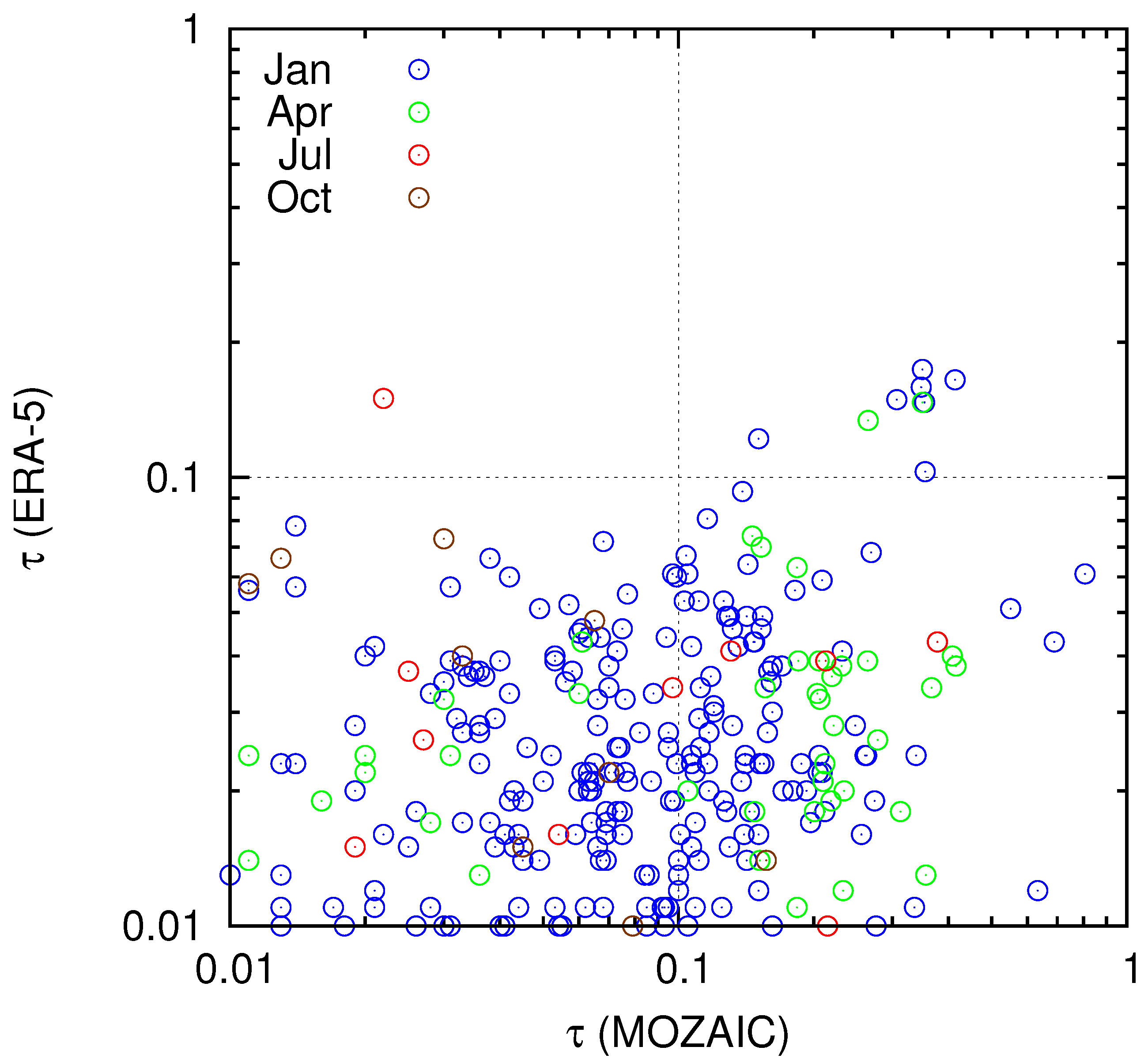
The Schmidt-Appleman criterion rules only contrail formation but not its persistence. For a contrail to exist more than a few minutes, and thus to be relevant to climate at all, it needs to be formed in an ice-supersaturated region (ISSR), that is, the ambient relative humidity with respect to ice, , must exceed unity (or 100%). Thus we compare now the measured from MOZAIC with the corresponding data from ERA-5. The result is presented in Figure 2 as a scatterplot and the degree of agreement between the data sets is shown in the lower half of Table 1. This comparison is, unfortunately, quite discouraging. The plot shows data pairs scattered all over the place, with only a weak indication of concentration of the points to the diagonal line. The entries of the contingency table (lower part of Table 1) and the corresponding ETS values confirm that the degree of agreement between the two data sets is quite low. Here we have at least a weak coherence in winter and spring with ETS values of and , respectively, but in the other seasons the relation is mostly random, although the computed slightly positive numbers are statistically significant. But this is merely the fortunate result of having a large number of cases.
Thus, the summary of this analysis is that while contrail formation can be forecasted quite reliably, their much more important property of persistence cannot currently be predicted reliably.
3.1.2. The Instantaneous Radiative Forcing
Figure 3 shows cumulative distribution functions (cdf) of instantaneous radiative forcing (iRF) for all cases where persistent contrails are diagnosed by MOZAIC, for the four months considered (colour coded) and separately for MOZAIC and the corresponding ERA-5 interpolated grid and time points. Please note that these curves refer to the mentioned random samples and not to all data. The most general observation is that cooling contrails (negative iRF) occur rarely, in less than 20% of the cases. Rather the cdfs rise steeply at zero and small positive iRF values which shows that most persistent contrails in the data sets have a slightly positive warming effect up to 10 W/m. The sample mean values plus/minus one standard deviation of iRF for the four months (01, 04, 07, 10) are in the MOZAIC data W/m and in the ERA-5 data W/m. That is, the iRF tends generally to higher values in MOZAIC than in ERA-5. As stated in the methods section, the only difference in the calculation is that we use the measured humidity and temperature for the radiation calculation in the MOZAIC case, which then translates into differences in the optical thicknesses. It turns out that these MOZAIC optical thickness values are often larger than their reanalysis counterparts, as Figure 4 demonstrates.
3.1.3. Comparison with EMAC Data
For April 2014 we have a sample of 660 matched data points for comparison. They cover a longitude range from 83 W to 138 E and extend in latitude from 14 N to 70 N. The temperature ranges from about 207 to 239 K, the model has a slight negative bias (mean difference) of K relative to the observations, with a standard deviation of K. For the relative humidity with respect to ice there is an average positive model bias of 13–14% (RHi percent, with standard deviation of 24%), although MOZAIC data have much higher maximum values than EMAC: the MOZAIC maximum is 150%, that of EMAC is 113%, but already the 3rd quartile is smaller for MOZAIC than for EMAC, 68% vs. 84%. Obviously there are many points in the EMAC data with RHi just around saturation, whereas MOZAIC, although showing some very high values, has the bulk of data with low RHi values. Note that the temperature bias is too small to explain the bias in relative humidity; there must be a bias in absolute humidity as well. The comparison for the water vapour volume mixing ratio suffers from an outlier in the EMAC data. If this outlier is removed, we find, in accordance to the results regarding RHi, a positive bias of 15 ppmv (with a standard deviation of 62 ppmv) of the EMAC data with reference to MOZAIC.
In spite of these biases the prediction of contrail formation would be quite successful with the EMAC data. A plot like Figure 1 to compare the pairs of looks as promising as in that figure (not shown), and indeed, the corresponding ETS is . But, unfortunately, the prediction of contrail persistence would be almost random with an ETS of . We see that EMAC with dynamics specified by using ECMWF meteorological fields as time dependent boundary conditions, has not better contrail formation and persistence prediction capabilities than the ECMWF model itself.
3.2. Case Studies
Let us begin with the case of 25 August 2008. This is a short story. We find that at the position and time when ACTA detected very strong contrails ERA-5 confirms the validity of the Schmidt-Appleman criterion with a of about , but is far from ice supersaturation with . This miss is not just a question of an error of a few degrees or a temporal mismatch of an hour or so. In fact, there is no ISSR closer than 10 in both longitude and latitude directions. For this case ERA-5 predicts short-living contrails where ACTA found very strong persistent ones.
Fortunately the case of 15 May 2009 is more yielding. The Schmidt-Appleman criterion is fulfilled with and there is an ISSR at the time and position of the contrail (Figure 5). However, the degree of ice supersaturation ERA-5 indicates is low (Figure 5, right panel); slightly exceeds 100% which has consequences for the estimate of the optical properties of the contrail. While the ACTA data indicate an optical thickness between around and , the contrail as predicted from ERA-5 data would perhaps just be visible under very clear conditions with an optical thickness between and (Figure 6, left). Consequently, the estimated iRF using ERA-5 data is with less than 1 W/m much smaller than what the ACTA data suggest, more than 55 W/m (Figure 6, right).
Although this looks discouraging, let us consider the meteorological situation for 15 May 2009 a bit closer. We identify the altitude of the contrails with the 225 hPa isobaric surface. At the location of the contrail there is a local minimum in the temperature field (215 K, Figure 7, left), which implies a local minimum in water vapour saturation pressure which hence favours the formation of ISSRs. The vertical air motion is relatively fast upward, about Pa/s (or about 5–6 cm/s, Figure 7, right). These circumstances promote not only ice supersaturation but also cirrus formation and indeed the contrail is found close to the western edge of a cirrus cloud that is embedded in a more extended cirrus field in the upper troposphere (Figure 8, left). Right at the position of the contrails there is a local maximum of upward motion. The contrail is in tropospheric air, but the dynamic 2-PVU tropopause is nearby to the west, perhaps 40 km (Figure 8, right). On the 200 hPa surface the PV does already exceed 2 PVU at the coordinates of the contrails; obviously these two contrails are indeed situated in the uppermost troposphere, directly beneath the dynamic 2-PVU tropopause. The upward motion encounters a barrier and is thus accompanied with a relatively strong (horizontal) divergence of 30 to more than s (Figure 9, left), which is typical for ISSRs but untypical for non-ISSRs [Table 1 of [5]]. The relative vorticity has a very strong gradient at the time and position of the contrails. On Figure 9, right, the contrails are situated just at the boundary between cyclonic and anticyclonic rotation. It seems that these Big Hits are situated at the top of an anticyclonic vortex that moves eastward. At 200 and 225 hPa the anticyclonic system is narrow. The vorticity in this anticyclonic system has at 1600 UTC quite large negative values that are again typical for ISSRs, around s, but the values at the contrail location increase steeply while the whole system moves west. At 1900 UTC the location is in cyclonic rotation and belongs to the stratosphere [or perhaps better, the extra-tropical transition zone, [28]]. Accordingly, there is then a strong decrease of the relative humidity to substantial subsaturation.
The ACTA cases thus show an ambivalent picture. In one case (25 August 2008) the forecast and observation disagree seriously, but in the second case (15 May 2009) there are a number of features present at the location of the Big Hits that are typical for ice supersaturation, in particular the dynamic situation characterised by cold air, upward motion close to the tropopause, strong divergence and anticyclonic rotation. The strong discrepancy between the retrieved and forecasted optical thickness and hence instantaneous radiative forcing results from the very small supersaturation in the reanalysis. The presence of nearby cirrus clouds in the model may yield an explanation, namely that supersaturation has been consumed by cirrus formation and growth. If cirrus formation takes place too early in the model, supersaturation is consumed too early as well and then there is not enough water to form thick contrails.
4. Discussion
4.1. Statistical Stability
In order to avoid effects of autocorrelation in the data analysis we selected randomly about 1% of the flight data to determine the entries in the contingency table. These entries are thus random numbers and the resulting ETS is random as well. If we had another random sample, the values would differ. Here we study how variable the numbers are when many samples are drawn. For this purpose we use all data of April 2014. From these 216,809 data we draw 1000 samples of size 2000 (i.e., ) and determine for each sample the ETS values for both the Schmidt-Appleman criterion and for supersaturation. From the resulting 1000 ETS values we determine their statistical properties. We obtain the following results:
- For the Schmidt-Appleman criterion we get an ETS range from to , the interquartile range is to , the mean value plus/minus one standard deviation is .
- For ice supersaturation we get an ETS range from to , the interquartile range is to , the mean value plus/minus one standard deviation is .
When we use all data, the corresponding ETS values are and , respectively, quite close to the sample mean. The entries in Table 1 are , which is close to the mean as well, and , which is in the upper quartile and thus not close to the mean.
4.2. Spin-Up Effects
Ice supersaturation was introduced in the ECMWF forecast system in 2006 [29], but only three years later in the analysis system. During this time the forecast ice supersaturation displayed spin-up in both extent and degree [30], leading to the recommendation to use forecasts with, say, 24 h lead time for applications that need supersaturation. However, since September 2009 this problem seems to be solved because the analysis system allows ice supersaturation as well. Ref. [31] show (in their (Figure 6, right)) that analyses and forecasts with 18 to 24 h lead time show quite similar statistics of relative humidity with respect to ice after September 2009. ERA-5 provides only short forecasts (18 h) so that tests of spin-up effects are confined to a comparison of 1 to 6 h lead time to 13–18 h lead time. We have tested these differences for the April data without finding significant changes relative to the evaluation presented above.
Ref. [31] show also that in-situ measurements of relative humidity from the CARIBIC measurement program [32] yields a RHi distribution with considerably higher values than both ECMWF analysis and forecast. This is probably due to the necessary assumption in the model that as soon a cirrus cloud forms all supersaturation within the cloud is immediately converted to ice (which actually can take hours, depending on crystal size distribution and number concentration). This might explain why the model indicates much thinner contrails than are found in the data sets.
4.3. Alternative Vertical Interpolation Procedures
So far we have used linear interpolation in p (pressure), which is not the best choice when a quantity like temperature rather varies linearly with altitude. We tested alternatives by replacing the interpolation in p with an interpolation in which is like a linear interpolation in geometric height (according to the barometric height formula). We also tested still another alternative weighting following [33], who use instead of p for vertical interpolation, where is the adiabatic coefficient for dry air (). This measure allows a better estimation of the tropopause pressure in data with coarse vertical resolution like reanalyses. We have tried both methods for a 1% sample of the April data: for the Schmidt-Appleman criterion we obtain , and for ice supersaturation . These are the same values that we had before in the p-system. Indeed it turns out that the alternative weights differ only very little from the weights in the linear p interpolation. The reason is that the pressure ratios of the ERA-5 levels (e.g., 300 to 250 hPa) are close to unity, and thus the functions , for instance, with or , are quite similar to .
4.4. The Relative Humidity Field
The results of this analysis seem to indicate that the relative humidity field in ERA-5 is unreliable, at least for the considered upper-tropospheric pressure levels. But this impression is not correct. In fact, the linear correlation between from MOZAIC and ERA-5 is relatively high for the drawn samples, ranging from for October to in July. However, high linear correlation is not enough for from ERA-5 to be a good predictor of contrail persistence. If we restrict the 4 samples to cases where both MOZAIC and ERA-5 find supersaturation, we find mean differences (ERA-5 minus MOZAIC) plus/minus corresponding standard deviations of for the four months, respectively; that is, the mean difference is in all cases negative, albeit insignificantly in July where ice supersaturation is rare, and as well insignificantly in October where the amount of flight data is lower than in the other months. These results indicate that ERA-5 underpredicts high humidity values and this is consistent with the result from above that the diagnosed optical thickness and resulting iRF values from ERA-5 are much smaller than the estimates based on the measurements. A possible reason for the underprediction is that the reanalysis provides grid-mean humidity values. When a grid box contains a cloud, the humidity in the cloudy part of the box is immediately (within one time step) reduced to saturation. The provided value of is a weighted mean: . When the humidity in the clear part of the grid box, , increases and surpasses a critical value, the cloud fraction C increases as well; this balancing effect inhibits the increase of grid mean humidity to observed maxima. For a successful forecast of contrail persistence it would be probably better to use the clear sky humidity values, . Although the clear-sky value can in principle be computed from and cloud fraction C, it is not a good strategy for our purpose, since becomes undefined when C approaches unity. Instead, one can simply try to choose instead of the grid-mean a C-weighted mean between the in-cloud value 1 and a maximum value that accounts for the threshold for homogeneous nucleation, given in Equation (4) of [29]. We tried both a linear (weights C and ) and a non-linear (weights and ) weighting; the resulting ETS values did not improve for contrail formation, but slightly for the prediction of persistence. However, with ETS values of for January, for both weightings for April, for July, and for October the resulting improvements are too low (and indeed within the statistical noise determined above) to base a successful contrail persistence prediction on this kind of clear-sky relative humidity.
5. Conclusions
In order to assess whether a promising strategy to eliminate a considerable share of contrail’s warming impact on climate is ready to be realized, namely to avoid the formation of Big Hits, which are contrails with a particularly large positive individual radiative forcing [15], we tested whether a state-of-the-art weather prediction model, represented by the ERA-5 reanalysis, is able to predict reliably (i) the formation of contrails, (ii) their persistence, and (iii) the magnitude of their instantaneous radiative forcing. As a representation of the actual conditions in the atmosphere we used measurements conducted on regular commercial passenger flights in the framework of the IAGOS/MOZAIC project. Additionally we used data from a global climate simulation from the EMAC model, extracted along the flight paths of a number of MOZAIC flights. These data have been analysed in a statistical fashion. Two case studies have been presented using strong contrail cases observed by satellites, that are available in the ACTA data.
It turns out that the thermodynamic condition for contrail formation can be predicted quite reliably, and this seems to work both for a pure weather prediction model and for a climate model in specified dynamics mode. The comparison of the results from the climate model simulation with the MOZAIC/IAGOS data shows that while the simulated temperature deviates only little from the measured one, the deviations in relative humidity are large. It is apparently the quality of the temperature prediction that leads to a promising result concerning contrail formation.
However, the problems of both weather and climate models to predict the relative humidity correctly, and in particular the underestimation of frequency and degree of ice supersaturation [see also [31]], lead to very low reliability in a forecast of contrail persistence. The underprediction of the degree of supersaturation leads to too low estimates of contrail optical thickness and thus to too low estimates of instantaneous radiative forcing. The results do not get substantially better with alternative vertical interpolation procedures or longer prediction lead times, nor with modified relative humidity values that might rather represent cloud-free areas than the standard grid-mean values that are provided in the reanalysis data.
We admit that this study may lack representativeness, since it covers only four months in one year and two case studies. We might have picked unlucky situations and the results might be better in other years or for other cases. Also using forecasts instead of reanalysis data may result in improved predictions of ISSR. The observations have their own uncertainties, but the statistical approach leads to cancellation of random errors. The determination of optical thickness and radiative forcing for the ACTA data is a problem when a contrail is located in cloudy background, because the determination of radiation fluxes for a cloud free environment turns out difficult. Thus there is a chance that the situation is better than what we have found here, but the necessary improvement is substantial.
Prediction of ice supersaturation at the right time and correct locations is basic to all operational contrail avoidance strategies. Some of them are quite complex and sophisticated, e.g., [34,35], but the current state of their concepts assume that the weather forecast is correct and that ISSRs will be where and when they are forecast. Before these concepts can be made operational, the prediction of ice supersaturation must become more reliable.
It seems that this reanalysis data has currently only limited capabilities for estimating real-world contrail formation along an aircraft trajectory. However, the ACTA data demonstrate that where thick contrails are found the model shows peculiar dynamical properties that are characteristic for ice supersaturation. This fact might offer new ways for prediction of Big Hits via general regression methods.
Author Contributions
Conceptualization, K.G. and S.M.; formal analysis, K.G.; data curation, S.M. and S.R.; writing–original draft preparation, K.G. All authors have read and agreed to the published version of the manuscript.
Funding
This work has received funding from the SESAR Joint Undertaking under grant agreement No 734161 and from the Research and Innovation Action ACACIA under grant agreement No 875036, both under the European Union’s Horizon 2020 research and innovation programme.
Acknowledgments
This work contributes to an ambition initiated by John Green and the Greener by Design working group of the Royal Aeronautical Society to take steps towards a real trial of reducing contrail formation by ATM measures. We thank Margarita Vázquez-Navarro (EUMETSAT) for provision of the ACTA data. Furthermore we thank Luca Bugliaro for critically reading the manuscript before submission and for his suggestions for improvement. A discussion with Robert Sausen on the methods was fruitful for the interpretation of the results. ERA-5 data are provided by the European Copernicus Data Service. Two anonymous reviewers helped to improve the paper. We are grateful for their positive assessment.
Conflicts of Interest
The authors declare no conflict of interest.
Appendix A. The Equitable Threat Score
There are several possibilities to describe how a certain dichotomous (e.g., 0/1, Y/N, black/white, etc.) feature in one set of data is reflected (or predicted) in another. Here we use contingency tables together with a certain measure of skill, the equitable threat score ETS. This and further skill scores are listed in [36].
A contingency table has 4 entries that are usually labelled hit (e.g., Y/Y), miss (Y/N), false alarm (N/Y), and correct negative (N/N). Let the numbers of these events be so that a is the number of hits, d is the number of correct negatives, and are the number of mixed results. The two datasets compare the better the larger is compared to and the degree of similarity can be expressed with skill scores. The nature of the data should guide the choice of the skill score. If the feature one is looking for is a rare event, d will be the largest number in the contingency table and this can feign a quite positive impression of the similarity of the two data sets, that is merely due to the rarity of the feature. It is thus appropriate to select a skill score that avoids to use d as much as possible. Furthermore, b and c should appear symmetrically in the formula if the same trust is given to both data sets or if one does not want to make one of the data sets the reference. The equitable threat score, with has the desired properties. for a perfect match (). For a completely random relation between the two data sets (), , and for a completely inverse relation () ETS is negative. In the case that N/N is predominant (i.e., the feature one is looking for occurs rarely), ETS approaches the threat score , that is, the predominant nature of d is filtered.
Monte Carlo experiments show that a purely random relation of the data gives an ETS of very nearly zero, since is quite large. Thus, all ETS values in the table indicate a statistically significant, albeit partly very weak agreement beween the data sets.
References
- Lee, D.; Fahey, D.; Forster, P.; Newton, P.; Wit, R.; Lim, L.; Owen, B.; Sausen, R. Aviation and global climate change in the 21st century. Atmos. Environ. 2009, 43, 3520–3537. [Google Scholar] [CrossRef] [Green Version]
- Grewe, V.; Dahlmann, K.; Flink, J.; Frömming, C.; Ghosh, R.; Gierens, K.; Heller, R.; Hendricks, J.; Jöckel, P.; Kaufmann, S.; et al. Mitigating the Climate Impact from Aviation: Achievements and Results of the DLR WeCare Project. Aerospace 2017, 4, 34. [Google Scholar] [CrossRef]
- Lee, D.; Fahey, D.; Skowron, A.; Allen, M.; Burkhardt, U.; Chen, Q.; Doherty, S.; Freeman, S.; Forster, P.; Fuglestvedt, J.; et al. The contribution of global aviation to anthropogenic climate forcing for 2000 to 2018. Atmos. Environ. 2020. [Google Scholar] [CrossRef]
- Schumann, U. On conditions for contrail formation from aircraft exhausts. Meteorol. Z. 1996, 5, 4–23. [Google Scholar] [CrossRef]
- Gierens, K.; Spichtinger, P.; Schumann, U. Ice supersaturation. In Atmospheric Physics. Background—Methods—Trends; Schumann, U., Ed.; Springer: Heidelberg, Germany, 2012; Chapter 9; pp. 135–150. [Google Scholar]
- Marenco, A.; Thouret, V.; Nedelec, P.; Smit, H.; Helten, M.; Kley, D.; Karcher, F.; Simon, P.; Law, K.; Pyle, J.; et al. Measurement of ozone and water vapor by Airbus in-service aircraft: The MOZAIC airborne program, An overview. J. Geophys. Res. 1998, 103, 25631–25642. [Google Scholar] [CrossRef]
- Gierens, K.; Schumann, U.; Helten, M.; Smit, H.; Marenco, A. A distribution law for relative humidity in the upper troposphere and lower stratosphere derived from three years of MOZAIC measurements. Ann. Geophys. 1999, 17, 1218–1226. [Google Scholar] [CrossRef]
- Mannstein, H.; Spichtinger, P.; Gierens, K. A note on how to avoid contrails. Transp. Res. Part D 2005, 10, 421–426. [Google Scholar] [CrossRef]
- Neis, P. Water Vapour in the UTLS—Climatologies and Transport. Ph.D. Thesis, Johannes Gutenberg- Universität Mainz, Mainz, Germany, 2017. [Google Scholar]
- Petzold, A.; Neis, P.; Rütimann, M.; Rohs, S.; Berkes, F.; Smit, H.; Krämer, M.; Spelten, N.; Spichtinger, P.; Nedelec, P.; et al. Ice-supersaturated air masses in the northern mid-latitudes from regular in situ observations by passenger aircraft: Vertical distribution, seasonality and tropospheric fingerprint. Atmos. Chem. Phys. 2020, 20, 8157–8179. [Google Scholar] [CrossRef]
- Hoinka, K.; Reinhardt, M.; Metz, W. North Atlantic air traffic within the lower stratosphere: Cruising times and corresponding emissions. J. Geophys. Res. 1993, 98, 23113–23131. [Google Scholar] [CrossRef]
- Schumann, U.; Graf, K.; Mannstein, H. Potential to reduce climate impact of aviation by flight level changes. In Proceedings of the 3rd AIAA Atmospheric Space Environments Conference, Honolulu, HI, USA, 27–30 June 2011; p. 3376. [Google Scholar] [CrossRef] [Green Version]
- Schumann, U.; Heymsfield, A. On the lifecycle of individual contrails and contrail cirrus. Meteorol. Monogr. 2017, 58, 3.1. [Google Scholar] [CrossRef]
- Teoh, R.; Schumann, U.; Majumdar, A.; Stettler, M. Mitigating the climate forcing of aircraft contrails by small-scale diversions and technology adoption. Environ. Sci. Technol. 2020, 54, 2941–2950. [Google Scholar] [CrossRef] [PubMed]
- Royal Aeronautical Society, Greener by Design; Annual Report 2018–2019; Royal Aeronautical Society: London, UK, 2019.
- Hersbach, H.; Bell, B.; Berrisford, P.; Biavati, G.; Horányi, A.; Muñoz Sabater, J.; Nicolas, J.; Peubey, C.; Radu, R.; Rozum, I.; et al. ERA5 Hourly Data on Pressure Levels from 1979 to Present. Copernicus Climate Change Service (C3S) Climate Data Store (CDS). Available online: https://cds.climate.copernicus.eu/cdsapp#!/dataset/10.24381/cds.bd0915c6?tab=overview (accessed on 14 June 2018).
- Petzold, A.; Thouret, V.; Gerbig, C.; Zahn, A.; Brenninkmeijer, C.; Gallagher, M.; Hermann, M.; Pontaud, M.; Ziereis, H.; Boulanger, D.; et al. Global-scale atmosphere monitoring by in-service aircraft—Current achievements and future prospects of the European Research Infrastructure IAGOS. Tellus B 2015, 67. [Google Scholar] [CrossRef] [Green Version]
- Jöckel, P.; Tost, H.; Pozzer, A.; Kunze, M.; Kirner, O.; Brenninkmeijer, C.; Brinkop, S.; Cai, D.; Dyroff, C.; Eckstein, J.; et al. Earth System Chemistry integrated Modelling (ESCiMo) with the Modular Earth Submodel System (MESSy) version 2.51. Geosci. Model Dev. 2016, 9, 1153–1200. [Google Scholar] [CrossRef] [Green Version]
- Vázquez-Navarro, M.; Mannstein, H.; Mayer, B. An automatic contrail tracking algorithm. Atmos. Meas. Tech. 2010, 3, 1089–1101. [Google Scholar] [CrossRef] [Green Version]
- Kox, S.; Bugliaro, L.; Ostler, A. Retrieval of cirrus cloud optical thickness and top altitude from geostationary remote sensing. Atmos. Meas. Tech. 2014, 7, 3233–3246. [Google Scholar] [CrossRef] [Green Version]
- Vázquez-Navarro, M.; Mayer, B.; Mannstein, H. A fast method for the retrieval of integrated longwave and shortwave top-of-atmosphere upwelling irradiances from MSG/SEVIRI (RRUMS). Atmos. Meas. Tech. 2013, 6, 2627–2640. [Google Scholar] [CrossRef] [Green Version]
- Vázquez-Navarro, M.; Mannstein, H.; Kox, S. Contrail life cycle and properties from 1 year of MSG/SEVIRI rapid-scan images. Atmos. Chem. Phys. 2015, 15, 8739–8749. [Google Scholar] [CrossRef] [Green Version]
- Gierens, K.; Vázquez-Navarro, M. Statistical analysis of contrail lifetimes from a satellite perspective. Meteorol. Z. 2018, 27, 183–193. [Google Scholar] [CrossRef]
- Jöckel, P.; Kerkweg, A.; Pozzer, A.; Sander, R.; Tost, H.; Riede, H.; Baumgaertner, A.; Gromov, S.; Kern, B. Development cycle 2 of the Modular Earth Submodel System (MESSy2). Geosci. Model Dev. 2010, 3, 717–752. [Google Scholar] [CrossRef] [Green Version]
- Roeckner, E.; Brokopf, R.; Esch, M.; Giorgetta, M.; Hagemann, S.; Kornblueh, L.; Manzini, E.; Schlese, U.; Schulzweida, U. Sensitivity of simulated climate to horizontal and vertical resolution in the ECHAM5 atmosphere model. J. Clim. 2006, 19, 3771–3791. [Google Scholar] [CrossRef]
- Schumann, U.; Mayer, B.; Graf, K.; Mannstein, H. A parametric radiative forcing model for contrail cirrus. J. Appl. Meteorol. Climatol. 2012, 51, 1391–1406. [Google Scholar] [CrossRef] [Green Version]
- Ebert, E.; Curry, J. A parameterization of ice cloud optical properties for climate models. J. Geophys. Res. 1992, 97, 3831–3836. [Google Scholar] [CrossRef]
- Hoor, P.; Gurk, C.; Brunner, D.; Hegglin, M.; Wernli, H.; Fischer, H. Seasonality and extent of extratropical TST derived from in-situ CO measurements during SPURT. Atmos. Chem. Phys. 2004, 4, 1427–1442. [Google Scholar] [CrossRef] [Green Version]
- Tompkins, A.; Gierens, K.; Rädel, G. Ice supersaturation in the ECMWF Integrated Forecast System. Q. J. R. Meteorol. Soc. 2007, 133, 53–63. [Google Scholar] [CrossRef] [Green Version]
- Lamquin, N.; Gierens, K.; Stubenrauch, C.; Chatterjee, R. Evaluation of Upper Tropospheric Humidity forecasts from ECMWF using AIRS and CALIPSO data. Atmos. Chem. Phys. 2009, 9, 1779–1793. [Google Scholar]
- Dyroff, C.; Zahn, A.; Christner, E.; Forbes, R.; Tompkins, A.; van Velthoven, P. Comparison of ECMWF analysis and forecast humidity data with CARIBIC upper troposphere and lower stratosphere observations. Q. J. R. Meteorol. Soc. 2015, 141, 833–844. [Google Scholar] [CrossRef]
- Brenninkmeijer, C.; Crutzen, P.; Boumard, F.; Dauer, T.; Dix, B.; Ebinghaus, R.; Filippi, D.; Fischer, H.; Franke, H.; Frieß, U.; et al. Civil aircraft for the regular investigation of the atmosphere based on an instrumented container: The new CARIBIC system. Atmos. Chem. Phys. 2007, 7, 4953–4976. [Google Scholar] [CrossRef] [Green Version]
- Reichler, T.; Dameris, M.; Sausen, R. Determining the tropopause height from gridded data. Geophys. Res. Lett. 2003, 30, 2042. [Google Scholar] [CrossRef] [Green Version]
- Rosenow, J.; Fricke, H. Individual condensation trails in aircraft trajectory optimization. Sustainability 2019, 11, 6082. [Google Scholar] [CrossRef] [Green Version]
- Avila, D.; Sherry, L.; Thompson, T. Reducing global warming by airline contrail avoidance: A case study of annual benefits for the contiguous United States. Transp. Res. Interdiscip. Perspect. 2019, 2, 100033. [Google Scholar] [CrossRef]
- Kästner, M.; Torricella, F.; Davolio, S. Intercomparison of satellite-based and model-based rainfall analyses. Meteorol. Appl. 2006, 13, 213–223. [Google Scholar] [CrossRef] [Green Version]
Figure 1.
Comparison of contrail formation conditions expressed as relative humidity in the exhaust plume in the moment when the temperature reaches , for MOZAIC (x-axis) and the corresponding ERA-5 data (y-axis). The seasons are plotted with intuitive colours: winter (January) blue, spring (April) green, summer (July) red, and fall (October) yellow. Contrails are possible when . Negative signifies conditions warmer than the maxmimum temperature where contrails are possible (that is, the plume does not get as cold as ).

Figure 2.
Comparison of relative humidity with respect to ice for MOZAIC (x-axis) and the corresponding ERA-5 data (y-axis). Colours are as in Figure 1. Contrails are persistent when .
Figure 2.
Comparison of relative humidity with respect to ice for MOZAIC (x-axis) and the corresponding ERA-5 data (y-axis). Colours are as in Figure 1. Contrails are persistent when .

Figure 3.
Cumulative probability distributions of instantanous radiative forcing of contrails for the four seasonal mid-months in 2014: January, April, July and October, both for MOZAIC data (solid lines) and the corresponding times and grid points in ERA-5 (dashed).
Figure 3.
Cumulative probability distributions of instantanous radiative forcing of contrails for the four seasonal mid-months in 2014: January, April, July and October, both for MOZAIC data (solid lines) and the corresponding times and grid points in ERA-5 (dashed).
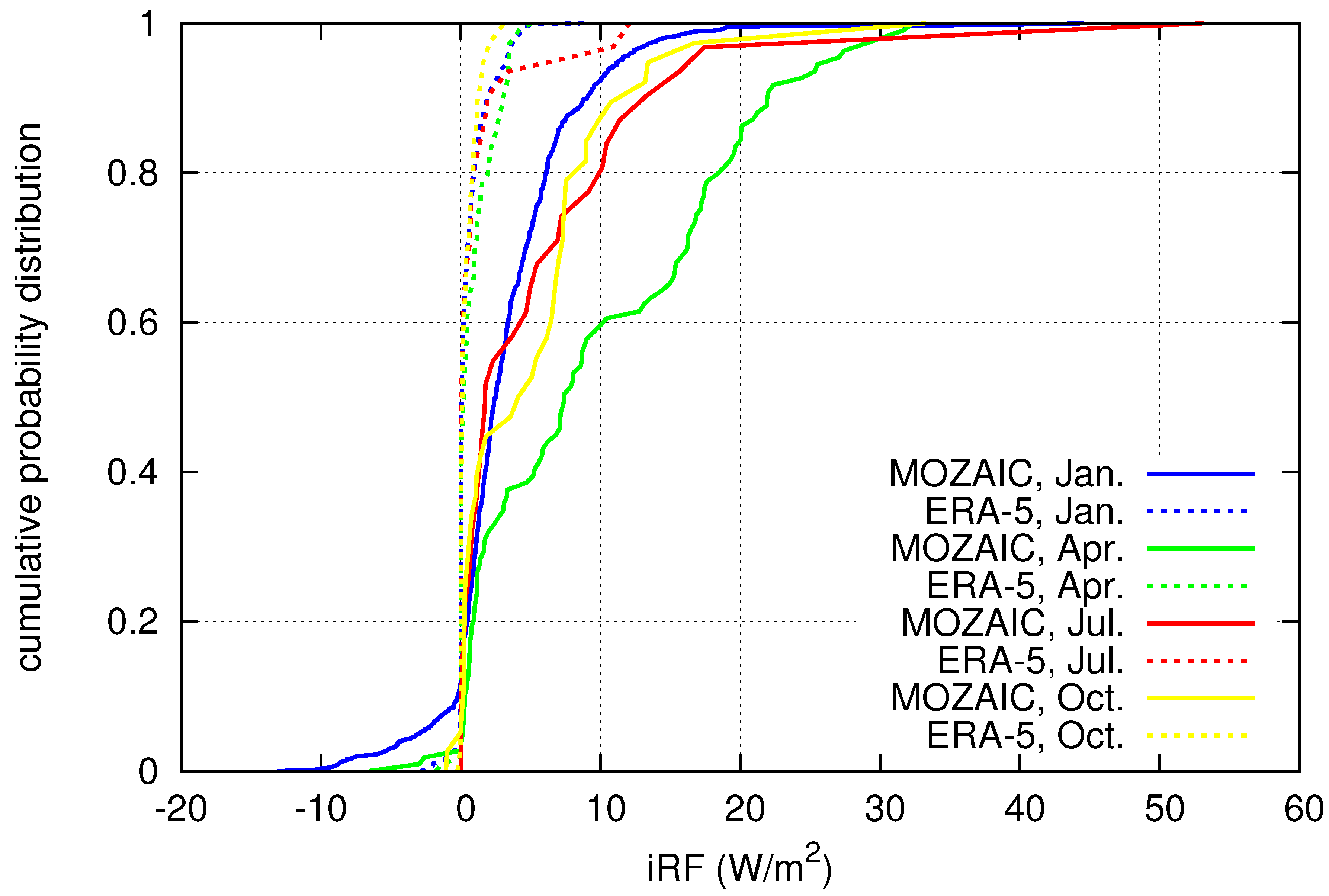
Figure 4.
Scatterplot of optical thickness values for persistent contrails that occur in both MOZAIC (x-axis) and ERA-5 (y-axis). Colour coding as before for the four months.
Figure 4.
Scatterplot of optical thickness values for persistent contrails that occur in both MOZAIC (x-axis) and ERA-5 (y-axis). Colour coding as before for the four months.

Figure 5.
(Left): Field of over a part of the Atlantic on 15 May 2009 at 18:00 UTC on the 225 hPa pressure surface. The positions where contrails have been observed by ACTA between 17:40 and 18:30 are marked as black dots. indicates that contrail formation is possible. (Right): The field of relative humidity with respect to ice for the same situation. The dashed line marks the transition between sub- to supersaturation.
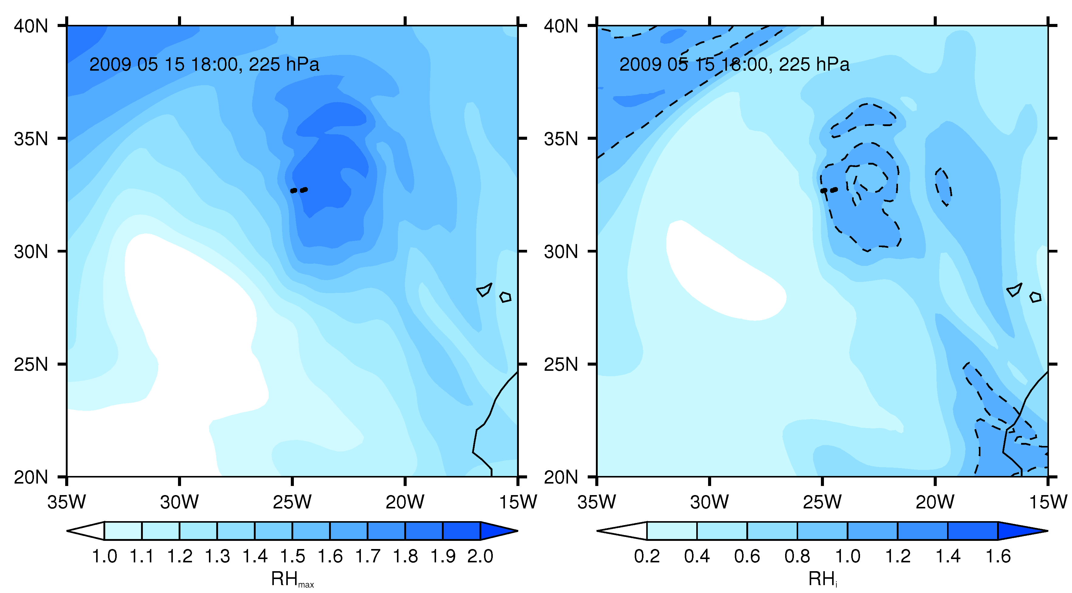
Figure 6.
(Left): Field of potential contrail optical thickness and (Right): Field of potential instantaneous radiative forcing for the situation of Figure 5.
Figure 6.
(Left): Field of potential contrail optical thickness and (Right): Field of potential instantaneous radiative forcing for the situation of Figure 5.
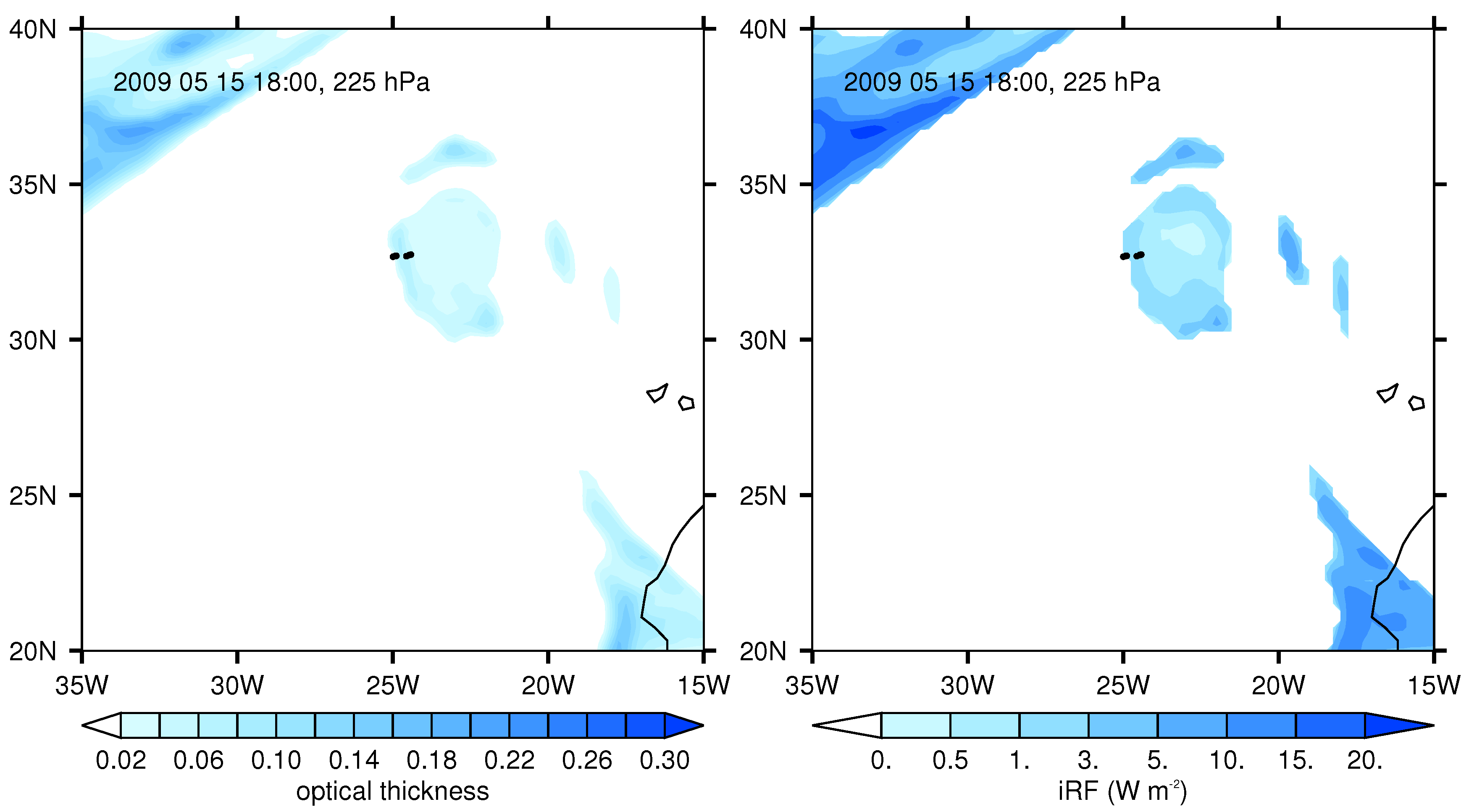
Figure 7.
(Left): Temperature field for the situation of Figure 5. The black line marks a temperature of C. (Right): Field of vertical velocity in pressure coordinates. Blue is upward, red downward.
Figure 7.
(Left): Temperature field for the situation of Figure 5. The black line marks a temperature of C. (Right): Field of vertical velocity in pressure coordinates. Blue is upward, red downward.
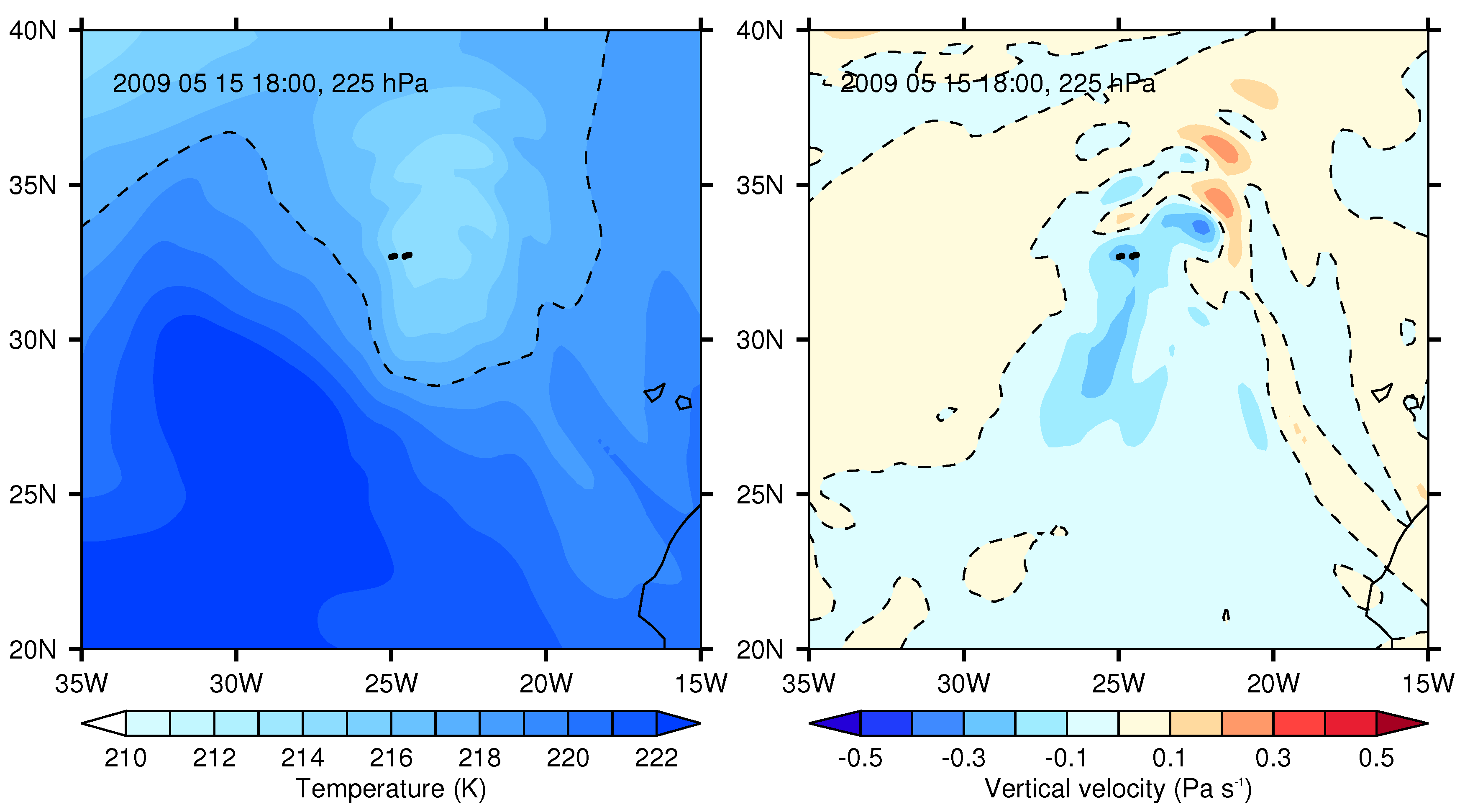
Figure 8.
(Left): Optical thickness of cirrus clouds for the situation of Figure 5. The black dotted lines represent the optical thickness integrated over the 200 to 300 hPa layer, while the coloured contours present the contribution of the layer around 225 hPa only. (Right): Field of potential vorticity (in PVU). The dashed line marks the 2 PVU surface, the dynamical tropopause or lower boundary of the tropospheric transition layer.
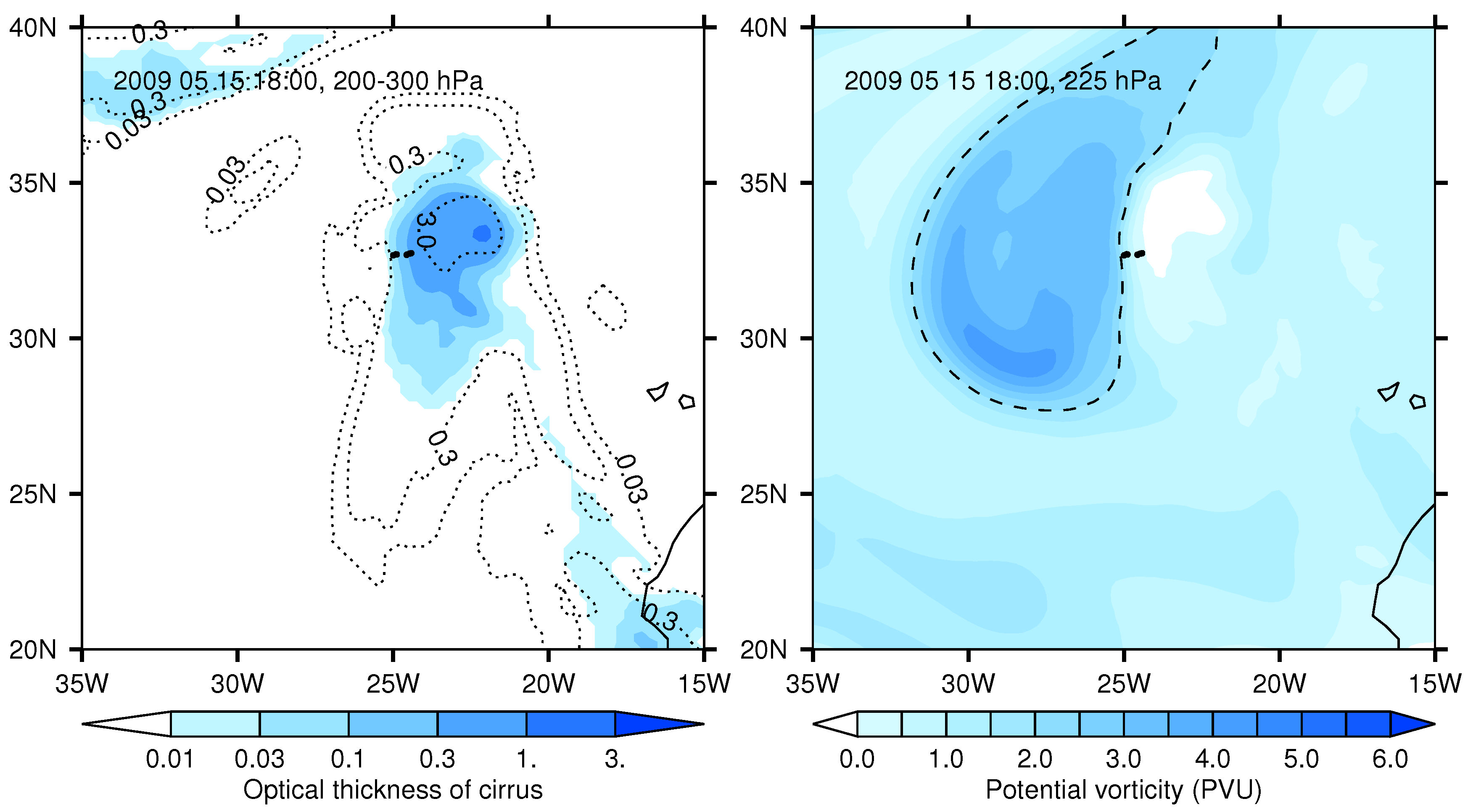
Figure 9.
(Left): Horizontal divergence for the situation of Figure 5. (Right:) Relative vorticity for the same case. The black dashed line marks in both cases zero, that is, the transition from convergence to divergence in the left panel and the transition from cyclonic to anticyclonic rotation in the right one.


Table 1.
Entries in contingency tables and equitable threat score (ETS); Y/N means that the feature exists in MOZAIC, but not in ERA-5. N is the number of data.
Table 1.
Entries in contingency tables and equitable threat score (ETS); Y/N means that the feature exists in MOZAIC, but not in ERA-5. N is the number of data.
| Month | N | Y/Y | Y/N | N/Y | N/N | ETS |
|---|---|---|---|---|---|---|
| SAC | ||||||
| 01 | 4706 | 3599 | 32 | 117 | 958 | |
| 04 | 2224 | 1726 | 8 | 103 | 387 | |
| 07 | 2552 | 679 | 13 | 319 | 1541 | |
| 10 | 1092 | 838 | 8 | 28 | 218 | |
| Ice-Supersaturation | ||||||
| 01 | 4706 | 34 | 157 | 199 | 4316 | |
| 04 | 2224 | 32 | 91 | 103 | 1998 | |
| 07 | 2552 | 9 | 35 | 102 | 2406 | |
| 10 | 1092 | 8 | 38 | 45 | 1001 | |
Publisher’s Note: MDPI stays neutral with regard to jurisdictional claims in published maps and institutional affiliations. |
© 2020 by the authors. Licensee MDPI, Basel, Switzerland. This article is an open access article distributed under the terms and conditions of the Creative Commons Attribution (CC BY) license (http://creativecommons.org/licenses/by/4.0/).
Share and Cite
MDPI and ACS Style
Gierens, K.; Matthes, S.; Rohs, S. How Well Can Persistent Contrails Be Predicted? Aerospace 2020, 7, 169. https://doi.org/10.3390/aerospace7120169
AMA Style
Gierens K, Matthes S, Rohs S. How Well Can Persistent Contrails Be Predicted? Aerospace. 2020; 7(12):169. https://doi.org/10.3390/aerospace7120169
Chicago/Turabian StyleGierens, Klaus, Sigrun Matthes, and Susanne Rohs. 2020. "How Well Can Persistent Contrails Be Predicted?" Aerospace 7, no. 12: 169. https://doi.org/10.3390/aerospace7120169
Note that from the first issue of 2016, this journal uses article numbers instead of page numbers. See further details here.