Article

Impact of Chinese and European Airspace Constraints on Trajectory Optimization

1
Institute of Logistics and Aviation, Technische Universität Dresden, 01069 Dresden, Germany
2
School of Electronic and Information Engineering, Beihang University, Beijing 100191, China
3
College of Civil Aviation, Nanjing University of Aeronautics and Astronautics, Nanjing 210016, China
*
Author to whom correspondence should be addressed.
Aerospace 2021, 8(11), 338; https://doi.org/10.3390/aerospace8110338
Submission received: 30 September 2021 / Revised: 1 November 2021 / Accepted: 2 November 2021 / Published: 10 November 2021
(This article belongs to the Collection Air Transportation—Operations and Management)

Abstract

:
Air traffic trajectory optimization is a complex, multidimensional and non-linear optimization problem and requires a firm focus on the essential criteria. The criteria cover operational, economical, environmental, political, and social factors and differ from continent to continent. Since air traffic is a transcontinental transport system, the criteria may also change during a single flight. Historic flight track data allow observation and assess real flights, to extract essential criteria and to derive optimization strategies to increase air traffic efficiency. Real flight track data from the Chinese and European air traffic show significant differences in the routing structure in both regions. For that reason, reference trajectories of historic ADS-B 24-h air traffic data in China and Europe have been extracted and analyzed regarding horizontal flight efficiency and the most restrictive criteria of trajectory optimization. We found that prohibited areas might be the most powerful reason to describe deviations from the great circle distance in the Chinese air traffic system. Atmospheric conditions, network requirements, aircraft types and flight planning procedures are similar in China and Europe and only have a minor impact on flight efficiency during the cruise phase. In a multi-criteria trajectory optimization of the extracted reference trajectories considering the weather, operational constraints and prohibited areas, we found that flown ground distances could be reduced by 255 km in the Chinese airspace and 2.3 km in the European airspace. The resultant reference trajectories can be used for further analysis to increase the efficiency of continental air traffic flows.

1. Introduction

An efficient air traffic network results from the superposition of sophisticated air traffic flow control and optimal individual trajectories. On a large scale, the air traffic flow management uses measures such as ground delay programs (GDP), re-routings or speed adjustments to optimize the air traffic flow [1]. On a small scale, single trajectories are optimized considering conflictive objectives for the sake of a sustainable and competitive transportation system recommended by the International Civil Aviation Organization (ICAO). This single trajectory optimization is going to be implemented in the framework of Trajectory Based Operations (TBO) as Reference Business Trajectory (RBT) until 2035, which was created by the Single European Sky (SES) Initiative [2].
The commercial air transport system has to comply with legal requirements which are declared in the Implementation Rules for Flight Operations (IR-OPS) [3]. Specifically, lateral path restrictions are defined in worldwide published route availability documents [4,5], available cruising pressure altitudes and aircraft mass constraints are regulated by ICAO in Doc. 4444 (Procedures of Air Navigation Services, Air Traffic Management) [6]. Furthermore, ICAO’s slot and Flight Level Orientation Scheme define airway and airport slot allocation in occupied air spaces and at busy airports [7].
Furthermore, the Radio Technical Commission for Aeronautics (RTCA) acts between stakeholders with competing interests and develops standards concerning critical aviation modernization issues. Their implemented performance standards significantly contributes to the safety, security, and overall health of an efficient aviation ecosystem. Specifically, SC-217, Aeronautical Databases and SC-186, Automatic Dependent Surveillance-Broadcast (ADS-B) recommends standards for the use, dissemination and archiving, as well as requirements on accuracy of aircraft flight track data. Thereby, RTCA attaches a great importance to being aligned with recommendations defined by the ICAO, and supports the goals set by SESAR, especially the Single European Sky (SES).
Additionally, political issues influence today’s flight planning and flight execution and thereby sometimes limit flight efficiency. These political instruments may define national airline policies and air traffic control methods with an impact on both the air traffic flow and single trajectory operations. These operational constraints change in time and space. For example, on average, military areas are blocking only a few per cent of European air space (see Figure 1), whereas the military controls 80 % of Chinese airspace [8]. In Europe, 25% of all flights are military flights [9].
The legal requirements and political boundary conditions lead to significant differences in flight planning and flight execution from continent to continent. From this it follows that trajectory optimization is more than a flight performance calculation.
Moreover, the distribution of knots (airports) within the network, their connectivity and the transport demand, compared to a usual aircraft capacity, strongly influences the efficiency of the network. Whereas Europe benefits from a relatively equal spatial distribution of airports, Asia suffers from hotspots with a high density of airports and areas with low air traffic activity. In Europe, large airlines (e.g., Lufthansa) act as network carriers by collecting long-haul passengers to hub airports and transporting them in large aircraft. In Asia, even the demand for short point to point connections (e.g., Shanghai to Beijing) already requires wide-body aircraft with high passenger capacity.
In this study, significant reference trajectories are extracted from real flight tracks (collected by radar data) and compared between China and Europe. The most likely trajectories are compared with optimized trajectories, considering as many operational constraints as possible. The differences in flight execution between both continents are going to be explained by operational conditions and typical weather conditions.

State of the Art

Besides these operational constraints, trajectory optimization relies on a precise flight performance model considering all forces of acceleration. Even if the equations of rotation are neglected in trajectory optimization, the three degrees of freedom aircraft model still induces six nonlinear first-order differential equations of motion. The aircraft performance model has to calculate and follow multi-criteria target functions for speed and altitude to be used as a trajectory optimizer. In advance, the conflicting goals on trajectory optimization, namely an increase in safety, economic efficiency and environmental compatibility, have to be transferred into key performance indicators (KPI) and quantified for each flight.
For this purpose, the flight performance model SOPHIA (Sophisticated Aircraft Performance Model) is used. SOPHIA is based to a large extent on purely physical laws, considers all forces of acceleration and uses the methodology published in [10]. Coefficients that cannot be estimated without aircraft-specific aerodynamic properties, such as drag polar and the maximum available thrust as a function of altitude and speed, are obtained from the open-source flight performance model OpenAp [11].
For extracting reference trajectories from flight track data, a cluster analysis is used. In this process, similar trajectories are grouped into clusters (i.e., points with similar characteristics) and reference trajectories are identified [12]. The goal of clustering is to divide data points into groups (clusters) so that objects of one group are as similar as possible and objects of different groups are as dissimilar as possible. Usually, multiple characteristics are used in cluster analysis. Cluster methods and their algorithms thus belong to the multilateral analysis methods [13].
There are different possibilities and variants to combine data points of a data set into clusters (cluster analysis) [14,15,16,17]. The algorithms of the various clustering methods differ mainly in the group definition, the complexity of the algorithms and the allowance of outliers [18], i.e., data points that are not assigned to a cluster. Similarity groups (clusters) of a method do not have to be similar in the sense of other methods. Cluster methods can be divided into hierarchical, partitioning, density-based, and some other, less common methods. The selection of a clustering method requires suitable modelling or determination of the similarity between data points. Depending on the modelling, the groups or clusters can have different sizes, shapes and densities, as well as be nested within each other.
On the one hand, partitioning (i.e., centre-based) clustering methods assign each cluster at least one object or data point and each object is assigned to exactly one cluster. For these methods, the number of clusters must be defined in advance. One of the most important partitioning clustering methods is the K-Means algorithm [19]. The prerequisite for the application of a partitioning method is the definition of the objects as points in an n-dimensional Euclidean vector space (real vector space with the scalar product). For the definition of similarity, the Euclidean distance (distance between two points in the vector space) is used.
Another partitioning cluster method, the fuzzy C-Means algorithm, calculates a degree of membership in a cluster for each data point [20]. When shifting the cluster centres during the calculation, distant objects with a low degree of membership have less influence on the shift than close objects. Thus, a relatively soft cluster assignment is achieved, since every point belongs to every cluster to a certain degree [20]. A big advantage of partitioning methods is that the clusters are not fixed during the calculation, so they can be dissolved and rearranged again and again and the objects can change their affiliation to a cluster during the shifting of the cluster centres. Disadvantages of partitioning methods are that the results are influenced by the increased reordering of the objects and that the starting position of the cluster centres or centroids is chosen randomly or subjectively and thus strongly influences the final result. Another disadvantage is that a complete application of the algorithm until the end of the enumeration is very computationally and memory intensive [20].
On the other hand, hierarchical clustering methods construct a sequence of partitions of the total object set. In contrast to the partitioning cluster methods, this set is not decomposed, but a hierarchy of clusters is constructed from the objects, from which a cluster structure can be derived. On one side you get a cluster with all objects and on the other side exactly as many clusters as you have objects [21]. For example, in agglomerative clustering methods, the clusters are merged further and further, using the Euclidean distance as a distance measure. Thereby, several fusion methods differ in the definition of the fusions, deciding which clusters are combined. Hierarchical clustering methods are highly flexible since complex distance measures can be combined. Furthermore, the result of the methods is always a cluster hierarchy, which allows substructures. However, in contrast to partitioning clustering methods, several clusters are produced as a result instead of a single one, resulting in high analysis effort. In addition, clusters are created from individual data points that have no similarities to others (outliers), which consist of only one or very few data points. This makes the model analysis more difficult for the user. Furthermore, once clusters have been formed, they can no longer be changed and individual data points can no longer be exchanged.
Third, density-based clustering methods calculate clusters according to the principle that objects are grouped in an n-dimensional space that is located close to each other. The clusters are separated from each other by areas with objects of lower density. For this purpose, parameters are set that define the distance measure as well as a minimum number of objects to form a cluster. An environment is dense if the minimum number of objects is reached or exceeded within the defined distance. A cluster is then formed from neighbouring dense environments. Density-based algorithms automatically detect data points or objects that do not fit into any of the clusters formed, so-called outliers. If outliers occur frequently, this is referred to as noise. Density-based algorithms sort them out and separate them from the formed clusters. The most important methods are the Density-Based Spatial Clustering of Applications with Noise algorithm (DBSCAN) [22], the Ordering Points To Identify the Clustering Structure algorithm (OPTICS) [23] and the Maximum Margin Clustering [24]. The most used algorithm, the DBSCAN algorithm, is defined by two parameters, the ε -environment and M i n c [a.u.]. To form a dense environment, a fixed minimum number of objects M i n c must lie within a fixed radius ε [a.u.] of a data point, which is defined as a core point. Multiple dense environments with core points whose distance is maximum ε form a cluster (see Figure 2).
In density-based clustering methods, the number of clusters does not have to be specified in advance and the clusters can assume any shape and size. However, this complicates the evaluation and interpretation of the results. Furthermore, these algorithms can be used with arbitrary distance functions and, in contrast to the partitioning clustering methods (especially K-Means), no centre point has to be calculated (i.e., no geometric space is necessary). Furthermore, the algorithm detects outliers or noise and filters them out [12]. In contrast, density-based clustering methods have difficulty detecting clusters of different densities. If the radius ϵ is chosen too large, areas with outliers are sometimes detected as clusters. Sometimes the algorithm has difficulties defining the density in case the objects have a lot of attributes or features [22].
Aircraft trajectories are mathematical point-based objects that describe the change in position of aircraft. The geographical position data (i.e., longitude, latitude and altitude), mapped in x- and y-coordinates onto a European projection can be used to form clusters in two-dimensional space. For the selection of the distance function, the Euclidean distance is suitable. ADS-B data are a highly frequent snap-shot of fast-moving objects. From this follows the possibility of noise (i.e., data points that do not show similarities to others), which cannot be declared as outliers by hierarchical clustering or partitioning clustering methods. The Gaussian Mixture Model (GMM) Algorithm based on the Expectation-Maximization Algorithm (EM-Algorithm) and the DBSCAN can deal with outliers. In contrast to the GMM algorithm, The DBSACN can estimate the optimum number of clusters. For that reason, the DBSCAN is used in this study.
In aviation, density-based clustering methods have already established themselves for many different issues. For example, for the assessment of safety issues by detecting abnormal operations, clustering algorithms are very useful. Li et al. developed ClusterAD [25] and applied this cluster-based anomaly detection on historic flight track data to identify abnormal operations. Furthermore, Campbell et al. [26] extracted possible go-around criteria of landing aircraft by clustering historic flight track data and Sheridan et al. [27] identified abnormal aircraft behaviors during the approach phase using the DBSCAN Cluster algorithm. All these studies benefit from the advantage of DBSCAN as an unsupervised learning method. Therefore, the result does not depend on the reliance of pre-defined parameter thresholds or definitions of these parameter thresholds. In addition, DBSCAN makes it possible to dispense with a presumably conservative delimitation of different events, the quality of which can be strongly influenced by subjective expert opinions [27]. For the same reason, Verdonk et al. [28] shares an efficient method to identify traffic flows (clusters of single aircraft trajectories) using DBSCAN. Ling et al. [29] provides a kernel-based DBSCAN algorithm to analyze the passenger behavior in civil aviation. Lee et al. [30] detects anomalous behaviours of aircraft engines in recorded flight data (FDR) to enable an improvement of airline maintenance operations. Unsupervised data-driven clustering analyses can be used for identifying significant impact factors on systems with many degrees of freedom. Therefore, feature extraction is a valuable instrument to focus on the right parameters in optimizations processes. Recently, Chakrabarti et al. [31] used data-driven clustering analysis to cluster trajectories in the approach phase considering air traffic control decisions. Furthermore, Saez et al. [32] used clustered trajectory prediction to develop optimal aircraft emergency trajectories. Olive et al. [33] summarize methods of data-driven trajectory analyzes and highlights the already mentioned the advantage of objectivity in data-based trajectory prediction and analysis. Promising methods from data science and artificial intelligence enable the possibility for controllers to predict and generate trajectories using only past observations [34]. This represents a significant step for a controller’s decisional support [35]. Zeng et al. [36] additionally highlighted benefits of the deep autoencoder and Gaussian mixture models to cluster aircraft trajectories in the Terminal Maneuvering Area (TMA).
In this article, we combine data-driven trajectory analyzes with our trajectory optimizer. The most recommended cluster algorithm DBSCAN is used to extract real reference trajectories of historical importance for two different busy air spaces. Subsequently the reference trajectories are optimized and assessed regarding historic detours. Those detours are investigated for their cause.
Using the clustered trajectories, historical reference trajectories and interpreted as the most flown trajectories in each continent. The idea of highly frequented routes has been also recommended by ICAO in the framework of the implementation of Area Navigation (RNAV) routes.
Air Traffic Flow Management (ATFM) aims to maximize Air Traffic Control (ATC) capacity and the air traffic volume [37]. Therefore, initial flight plans with primary airline intentions are balanced and sometimes rerouted in a pre-tactical phase of ATFM. Decision support for this task is provided by Traffic Orientation Schemes (TOS) which consist of traffic flow restrictions that are considered in flight plan optimization. In Doc 4444, ICAO recommends designing TOS in a way that direct routes are allowed whenever possible considering the highest possible flexibility, especially for long-haul flights [6]. For example, in Europe, TOS are used in the Route Availability Document (RAD). In the north-Atlantic region, TOS are defined in the North Atlantic Track Organised Track System (NAT OTS). RAD is published by Eurocontrol every 28 days together with the “Aeronautical Information Regulation And Control” (AIRAC) cycle. Therein, airway segments or single waypoints (i.e., flow elements) might be allowed, forbidden, or even mandatory to use. In 2001, ICAO recommended defining so-called Area Navigation (RNAV) trunk routes: In dense air spaces, aircraft are allowed to freely operate within a network of navigation beacons without navigating directly between these beacons, fulfilling a defined system capability [38]. Adopting this idea of trunk routes, we extract historic reference trajectories as a result of the clustering algorithm.
The article is structured as follows: Section 2 provides an overview of significant operational air traffic constraints in China and Europe and derives suspected main impact parameters for trajectory optimization in both regions. Section 3 focuses on continent-specific weather phenomena with suspected impact on trajectory optimization (despite political constrains). In Section 4 the methodology of the data analysis is described in detail and Section 5 provides the main findings of the clustered and analyzed historic flight track data. Section 6 provides a comparison of optimized and historic paths in both regions and highlights the significance of airspace constraints in China, which overcame the impact of weather-induced restrictions in the Chinese airspace. Finally, Section 7 provides a summary and conclusion of the main results.

2. Operational Constraints in China and Europe

The areas of investigation, eastern China and central-south Europe are similar in size, aircraft movements and inhabitants (Table 1). For this reason, they are well-suited for a comparison of clustered trajectories.

2.1. Chinese Constraints

Chinese airspace is composed of ten flightiInformation regions (FIR) (Shenyang, Beijing, Shanghai, Wuhan, Guangzhou, Sanya, Kunming, Chengdu, Lanzhou, Urumqi), 23 restricted areas and 176 prohibited areas [39]. Aircraft are not allowed to enter or cross restricted areas or prohibited regions [40,41]. In case restricted areas are available for temporal flight routes, the conditions are published 24 h beforehand for dispatchers to plan the flight [40]. Figure 3 indicates that most of the restricted areas are located in the eastern part of China, where the main air traffic also takes part.
In 2016, Chinese airport punctuality put it amongst the 20 worst airports in the world (Hangzhou with the worst Chinese on-time performance with 41%). For comparison, Haneda, the busiest airport in Tokyo, had an on-time performance of 92% [42]. There were various reasons for the poor on-time performance, including over-scheduling, weather and limited capacity airspace. A large number of military areas partly block more than 70% of eastern China’s airspace, while the airspaces are blocked on short notice and sometimes for long periods (in the order of magnitude of weeks). Luckily, around 30% of these military airspaces are open below 1000 m to ensure emergency service, such as for helicopters [42].
Flight planning in China is based on historical routes and their connectivity to hub airports. Dispatchers choose frequently used routes, but also check the weather patterns and often try to reduce the fuel consumption. All airline business models are also represented in Asia. Besides low-cost leisure carriers with limited service and low airfarse, business carriers are more sensitive to access time and punctuality.
In China, overfly charges are almost constant (see also Figure 3). They only differ in foreign and domestic airlines [40]. Furthermore, flying through the busiest area of responsibility (AOR) SANYA costs twice as much. Since these overfly charges are not publicly available for research purposes, we assume a rate of 1 € per kilometre in the AORs Hong Kong, Macau and Taiwan and 2 € per kilometre in SANYA AOR for foreign airlines. For domestic airlines, we assume 0.5 € per kilometre in Hong Kong, Macau and Taiwan and 1 € per kilometre in SANYA AOR. The actual kilometres flown shall be determined by the kilometres of the air route specified in the route chart published by the Civil Aviation Administration of China. For comparability with Europe, we focus on foreign airline charges.

2.2. European Constraints

In Europe, restricted airspaces play a minor role in air traffic operations. In fact, in December 2019, 55 Area Control Centers (ACCs) have already implemented so-called free route airspace (FRA) operations more or less completely. Airlines can file and operate along freely planed routes considering entry points, exit points and intermediate points. Full FRA operations within Europe are expected by 2024 [43]. Entry and exit points are located along the border of the Flight Information Regions (FIR). Sometimes, even in FRA, compulsory Air Traffic System (ATS) routes or directed segments are published in national route availability documents (RAD) or the Aeronautical Information Publication (AIP). However, 27 national air traffic control authorities from over 60 ACCs coordinate the airspace over Europe. Radio contact must be established with the ground station of each ACC flown through. ACCs vary greatly in their radar coverage and overflight charges. This fragmentation partly results in an airspace structure that is oriented towards national borders and sometimes hampers an efficient routing. In Europe, overfly charges C overfly [€] are very heterogeneously distributed in so-called charging zones (see Figure 1) and calculated by [44]
C overfly = U R · W F · D F .
For each zone, unit rates U R [€] are monthly adjusted and published by EUROCONTROL [44]. C overfly depend not only on the zone aircraft are flying through but also on the weight factor W F [a.u.]
W F = M T O W / 50
where the M T O W [kg] denotes the aircraft maximum take-off mass and by the distance factor D F [a.u.]
D F = D / 100
where D [km] denotes the great circle distance between the entry point (or airport) and the exit point (or airport) of the zone overflown. Since January 2020, the distance factor is calculated according to the actual flown route as known to the Network Manager [45].
Due to the civil-military integration of air traffic control, European air navigation service providers often not only control civil air traffic but also supralocal military air traffic. Therefore, air traffic can be controlled more flexibly and dynamically in a coordinated and joint use of airspace. Military airspace closures are adapted to the requirements of the armed forces and are initiated as rarely as possible. Furthermore, some military training flight operations can take place in parallel and with direct interaction with civil aviation. This optimises civil routing: flight routes are shortened because military restricted areas do not have to be flown around extensively [46].
Restricted and prohibited areas are defined in the AIRAC cycle [6] (Annex 15, Chapter 5) and are updated every 28 days. Since this information is not available for research purposes, we assume the prohibited areas as shown in Figure 1.

3. Weather Impact on Air Traffic in China and Europe

The high impact of atmospheric conditions on the air traffic system is considered by dispatchers in the flight planning phase for decades, because the weather does not only effect safety, efficiency and punctuality in the en-route phase of the flight but also cause delays and cancellations due to difficult conditions for airport operations [47,48]. Specifically, snow, sleet, and freezing rain combined with strong winds, low clouds, and reduced visibility may cause dangerous conditions in the Terminal Maneuvering Area (TMA) [47]. Furthermore, precipitation (liquid or solid) impacts the runway conditions and visibility. Crosswind conditions can hamper the ability of the aircraft to safely take off or land.
In the en-route phase, a low cloud ceiling can induce poor or no visibility of the sky. Wind direction and speed can change the course of aircraft with serious consequences. Heavy accumulations of ice, frost, and snow, as well as freezing rain or drizzle on aircraft surfaces, change the flow around the aircraft and thus its stability and controllability throughout the flight [48].
Some of those difficult atmospheric conditions are season-specific and might be predictable. Others prevail at least for several hours and thus can be considered in flight operations. For example, blizzards can be described as sustained winds with frequent gusts up to 16 m per second and large amounts of snow, which reduces the visibility frequently to less than 400 m). In the TMA, large amounts of ice and snow (more than 0.5 m) can also pull down trees and utility lines and therewith reduce the power and communication between aircraft and air traffic control [47].

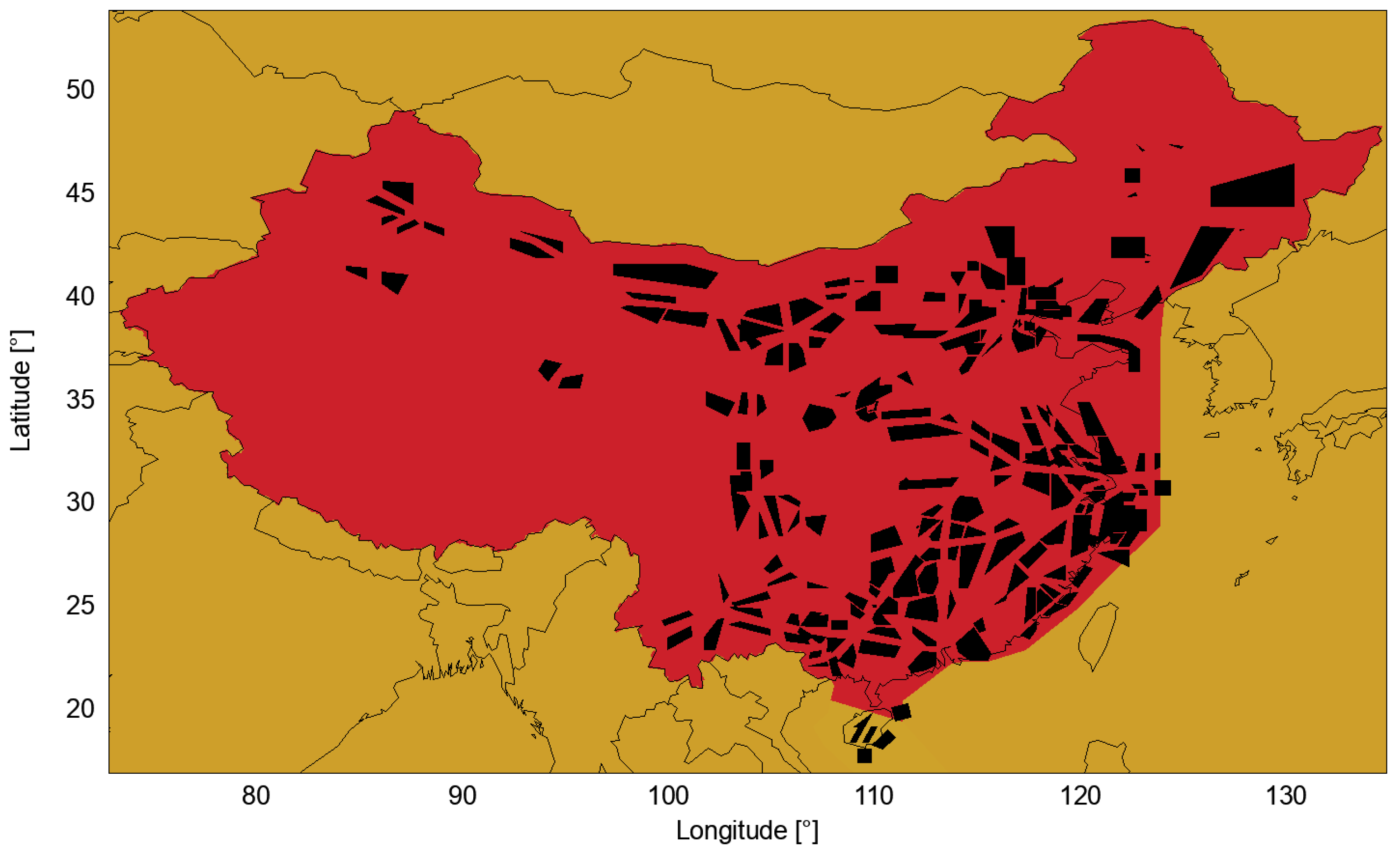
3.1. Chinese Weather Impact on Air Traffic

Typical weather conditions with impact on the air traffic route structure include monsoon rainfalls during summer from April to September in the Southern part of China [49,50]. On average, precipitation of 276 mm in June and 233 mm in July is measured in Guangzhou. These values are even higher in Hong Kong (323 mm in June), Shanghai (270 mm in June) and Shenzhen (327 mm in June) and Guangzhou (404 mm in June) [51]. Due to heavy rains, strong winds and severe turbulence appearance, these seasonal changes in precipitation reduce the ATM system capacity for relatively long periods, not only in the TMA but also in the en-route phase, by complicating the navigation performance [47]. Specifically, coastal areas are affected by spontaneous wind direction changes of up to 180 degrees and above-average clouds which have to be flown around [49].
Between May and December, south China is prone to typhoons, which are tropical cyclones in East and Southeast Asia, as well as in the northwestern part of the Pacific Ocean, formed in a powerful low-pressure area. Especially between July to September, the islands of Hong Kong and Taiwan and the coastal provinces of Guangdong and Fujian are faced with wind speeds of up to 55 m per second. These cyclones do not only complicate the navigation performance (strong wind speeds) but also lead to short-time severe rainfall and strong winds.
It is expected but not proven, that these seasonal weather occurrences have impact on lateral routing.

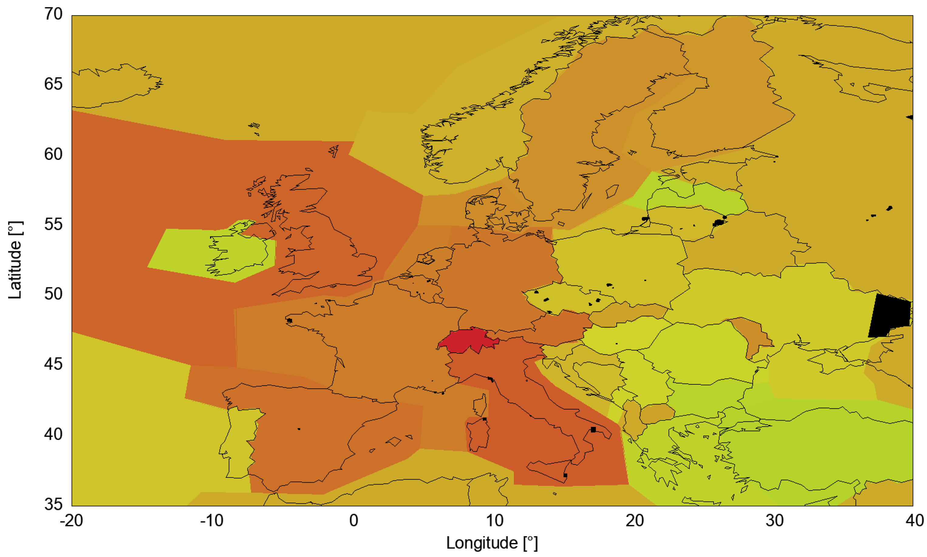
3.2. European Weather Impact on Air Traffic

Compared to China’s seasonal monsoon precipitation affecting air traffic, there are few typically European weather events with predictable impacts on air traffic, except for winter snowfall and frost. However, some local and short-term disruptions in Europe’s air traffic can be found in different weather phenomena causing limited visibility, severe thunderstorms, wind shear, and snowfall (Tafferner et al., 2010; Gerz et al., 2012) [52,53,54]. For example, in autumn, winter and spring, the mistral is a local cold, dry and often strong downdraft wind in France [55]. The resulting wind flows through the river valleys of the Rhön Mountains and is thereby constricted over a large area [55]. It can occur between the Western Alps and the Massif Central or between the Massif Central and the Pyrenees. In this area, a jet-like acceleration of the wind is possible. The mistral can occur abruptly and reach far into the western Mediterranean [55]. Bora also describes local, sometimes long-lasting, cold and gusty downdrafts on various coastal areas, especially between Trieste and the mouth of the Drim on the Croatian and Montenegrin Adriatic coasts. The bora usually occurs in winter. Individual gusts of these winds can reach peak speeds of up to 250 km/h west of the Velebit [55]. While the strong winds often affect airport operations, they rarely affect routing.

4. Data Analysis

High speeds, high cruising altitudes and the significant influence of the wind make it difficult to record a flight path by measuring the aircraft itself. For this reason, numerous methods have been established over the last decades to precisely record an aircraft trajectory so that it can be traced and evaluated later. The deviations between the methods have developed into a separate field of research. Precise FDR data, which are recorded in the aircraft’s own coordinate system, are rarely available to the research community for security reasons and to protect the personal rights of the flight crew. Although the observation of the flight in the earth-fixed coordinate system by means of ADS-B does not allow the availability of flight performance-specific data such as thrust, fuel flow or true air speed, this method provides a large amount of data through high-frequency transmission of the position data of each aircraft, which can be evaluated by the research community.

4.1. Automatic Dependent Surveillance Broadcast

Automatic Dependent Surveillance-Broadcast (ADS–B) is an advanced surveillance technology that combines an aircraft’s positioning source, aircraft avionics, and ground infrastructure to create an accurate surveillance interface between aircraft and ATC. With an appropriate ADS-B transponder installed in the aircraft, position and aircraft status data are broadcast periodically, called ADS-B out. This equipment is mandatory to cross many airspaces (e.g., in the US following Part 14 CFR 91.225). The signals can be received from other aircraft and ground stations at a distance of up to 200 NM (approx. 370 km) using SSR Mode S transmission, following range properties of the 1.090 MHz radio waves, and up to to 2000 NM (approx. 3700 km) if Low Earth Orbit (LEO) satellite navigation is used [56]. The aircraft system can create a traffic situation in its surrounding (Cockpit Display of Traffic Information) [56]. An advantage of ADS-B is, in contrast to ground-based surveillance systems in aviation, remote and mountainous areas can also be covered with surveillance functions.
In this study, the Chinese subset of ADS-B data is provided for research purposes by the Nanjing University of Aeronautics and Astronautics, which has a close relationship with Chinese aviation data provider VariFlight (https://www.variflight.com/, accessed on 20 March 2021).
The Chinese data set contains ADS-B flight parameter information of 13670 trajectories in the period from 21 November 2020 12:00 UTC+8 to 22 November 2020 23:59 UTC+8 from the Chinese and partially surrounding Asian region. At the end of November 2020, domestic air traffic in China was at 90% of pre-crisis levels, despite a global virus pandemic at that time [57]. The resulting baseline of available trajectory data is sufficient for extracting domestic reference trajectories in China.
The European data set is provided by the Open Sky Network (https://opensky-network.org/, accessed on 17 January 2021). The period chosen is Tuesday, 7 May 2019 10 a.m. to Wednesday, 8 May 2019 10 a.m., representing an average traffic-heavy period. The area of investigation is limited to longitudes from 10° West to 25° East and latitudes from 35° North to 55° North. The northern European region (of minor importance due to the lower volume of air traffic) is not included to limit the enormous amount of data. Only aircraft in cruise flight is analyzed above 24,500 feet (upper airspace), which corresponds to an altitude of 7467.6 m. In total, the ADS-B data set contains data of approx. 38,800 different trajectories with an update rate per trajectory of 1 s.
Both data sets provide the following information with relevance for the cluster analysis: transponder ID [string], time [Unix time stamp], latitude [°], longitude [°], altitude [ft], heading [°], ground speed [kt], callsign [string] and a registration [string].
The technical performance of ADS-B technology can be evaluated by the indicators of accuracy, latency, integrity and continuity. The maximum deviations are defined by ICAO and prescribed by law for the European Organization for the Safety of Air Navigation (Eurocontrol) [58].
The accuracy is defined as the difference between the position sent in the ADS-B message and the true position of the aircraft. The absolute deviation of the measured position from the actual position must not exceed a radius of 150 m (in air spaces with 3 nautical miles separation) by 95%. In practice, depending on the global navigation system used, position data determined utilizing GNSS achieve deviations of less than 15 m (GPS and GALILEO) or less than 8 m (GLONASS) with a 95% probability [59].
Latency is the measured time delay between the position determined by the aircraft via GNSS and the reception of the ADS-B message. The latency is specified in milliseconds. The ADS-B message does not contain the time that was current at the position measured by GNSS, which is why the receiver can only record the time at which the ADS-B message arrives with its clock. The measured latency time thus has a significant influence on the accuracy of the position of the aircraft. The average latency is less than 0.1 s [59]. Thus, the position deviation at a speed of 154 m per second (approx. 300 knots) is less than 15.4 m [56]. This means that the maximum total delay time of fewer than 1.5 s specified by ICAO is undercut in 95% of all ADS-B messages and therefore complies with [60].
Integrity is the correctness of data and the correct functioning of a system. In ADS-B systems, integrity describes the probability that information is true, as well as the reliability with which false information is correctly detected by the ADS-B system. An ADS-B message from an approved ADS-B transponder may be false with a maximum probability of 101-5 per flight hour and must be detected by the system in less than 10 s [59].
Continuity describes the probability that the system will perform the function required of it without unforeseen interruption. The continuity of certified ADS-B transponders must be less than 2 × 10 4 per flight hour, which corresponds to an average failure interval greater than 5000 flight hours [58].

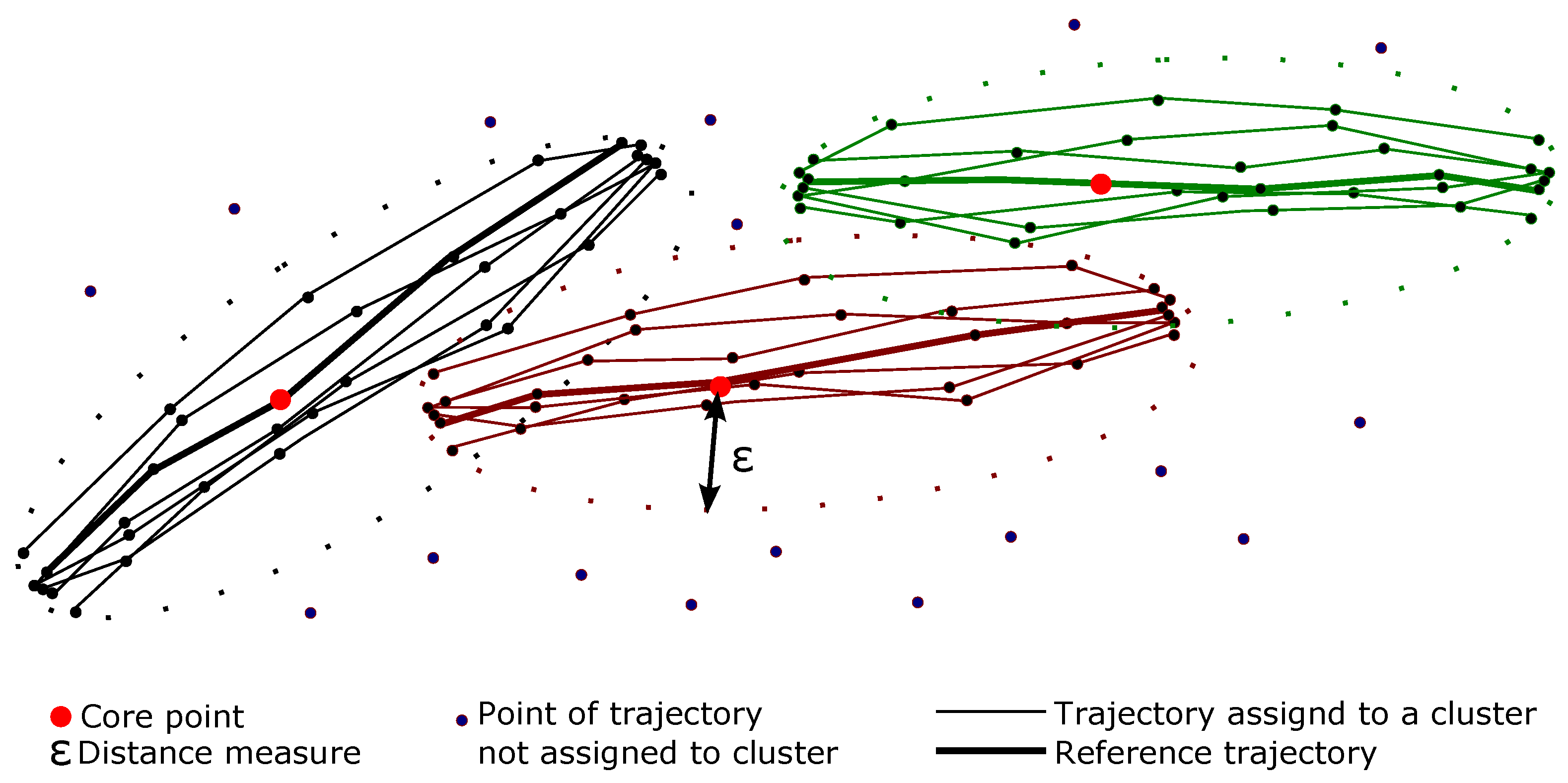
4.2. Clustering Flight Track Data

The cluster analysis has been done using the open-source air traffic data processing library Traffic [18]. For running a DBSCAN cluster analysis with acceptable computation time, the ADS-B aircraft position data are reduced to significant data points using the Douglas-Peucker-Algorithm with a maximum Hausdorff distance dimension between the original and the simplified curve ϵ = 0.5 [61]. After this step, each trajectory is represented by 15 data points, on average. The number of 15 data points per trajectory has been identified as a good compromise between calculation time and accuracy by [35]. Subsequently, all variables and objects with possible similarity characteristics are selected and the similarity or distance characteristic values of the data points are determined. These characteristic values might be adjusted iteratively to obtain the best solution. The results depend on the quality of the available data set as well as on the requirements for the classification of the clusters. For that reason, the aspired comparison of cluster results from two different data sets poses a challenge to the analysis. The problem is solved by using the same cluster algorithm for all data sets and by using algorithms for parametrization.
Similarity between objects ( o 1 , o 2 ) is defined by a distance or similarity function d i s t ( o 1 , o 2 ) or s i m ( o 1 , o 2 ) . For a distance function d i s t , the value d i s t ( o 1 , o 2 ) becomes smaller, the more similar two objects ( o 1 , o 2 ) are and vice versa [13]. Usually, a weighted euclidean distance
d i s t ( x j , x k ) = i = 1 n ( w i ( x j i x k i ) 2 )
is used, where ( x j , x k ) describe a pair of data points (objects), w i denote a weighting of the attributes ( x j i , x k i ) which which in turn represent the geographic coordinates longitude [°], latitude [°] and track [°] of the objects. The track, defined as path angle over ground compared to true North [°], has been unwrapped by replacing large numerical gaps between 359° and 1° by the complement [18]. Considering the track in cluster analysis separates similar trajectories with a track in the opposite directions. Furthermore, the following conditions must be fulfilled:
d i s t ( o 1 , o 2 ) = d R > 0
d i s t ( o 1 , o 2 ) = 0 for o 1 = o 2
d i s t ( o 1 , o 2 ) = d i s t ( o 2 , o 1 )
For the parametrization of ε and M i n c , the balanced ratio between the number of clusters and the number of accepted outliers must be found. Since the final aim of this clustering is the extraction of reference trajectories, the number and size of clusters should allow the definition of reference trajectories between important airports. For comparability, these parameters should be equal for both the Chinese and the European data sets. We found ε = 0.5 and M i n c = 10 yield is distinguishable reference trajectories and an acceptable number of outliers. The result of the cluster analysis are spatially grouped trajectories with similar tracks (compare Figure 4).

4.3. Extraction of Reference Trajectories

This study aims to identify and assess reference trajectories concerning efficiency. Therefore, within each cluster, the trajectory closest to all other trajectories of the cluster is identified as reference trajectory using the Euclidean distance (Equation (4)). The similarity between the attributes longitude [°], latitude [°], track [°], ground speed [m s 1 ] and altitude [m] is considered. Again, each reference trajectory is represented utilizing approximately 15 data points. This approach has the advantage that a real trajectory is identified as a reference for this cluster, which can be easily recalculated and optimized using a flight performance model.

4.4. Multi-Criteria Trajectory Optimization

Subsequently, the extracted reference trajectories are used as representatives and are analysed in more detail. First, the trajectories are modelled and assessed with a flight performance model SOPHIA. Second, the representatives are optimized and assessed with the Toolchain for Multi-criteria Aircraft Trajectory Optimization (TOMATO) [10,62,63,64] which includes the aircraft performance model SOPHIA for vertical optimization and the quantification of the emissions. Besides, typical input variables for trajectory optimization, such as city pair, aircraft type, engine type, payload, optimization function (i.e., minimum fuel burn, minimum time of flight, minimum contrail impact or multi-criteria optimization), the implemented key performance assessment in TOMATO allows a trajectory optimization and assessment. In TOMATO, the trajectory is optimized iteratively by assessing each interim solution regarding several key performance indicators (KPI).

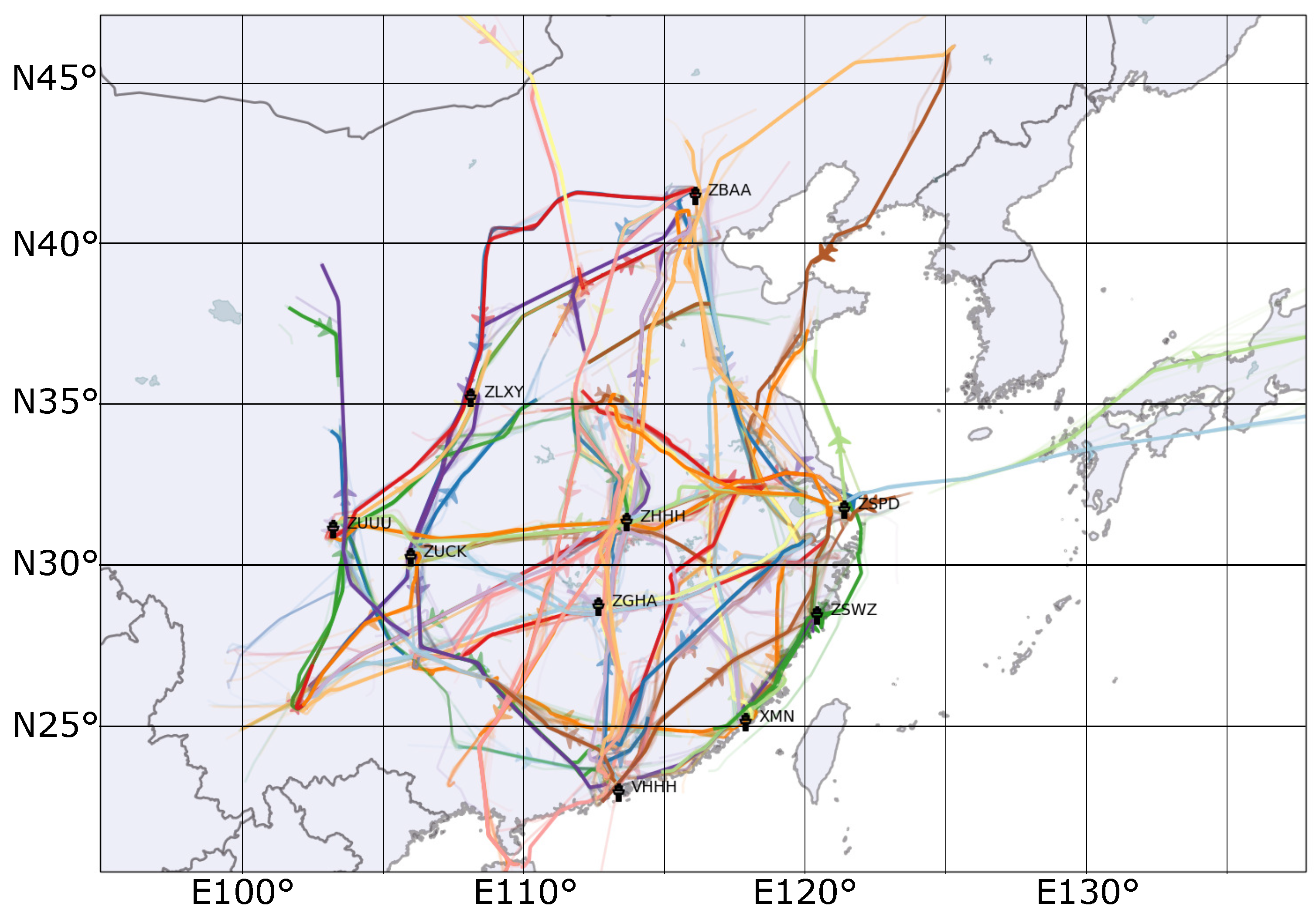
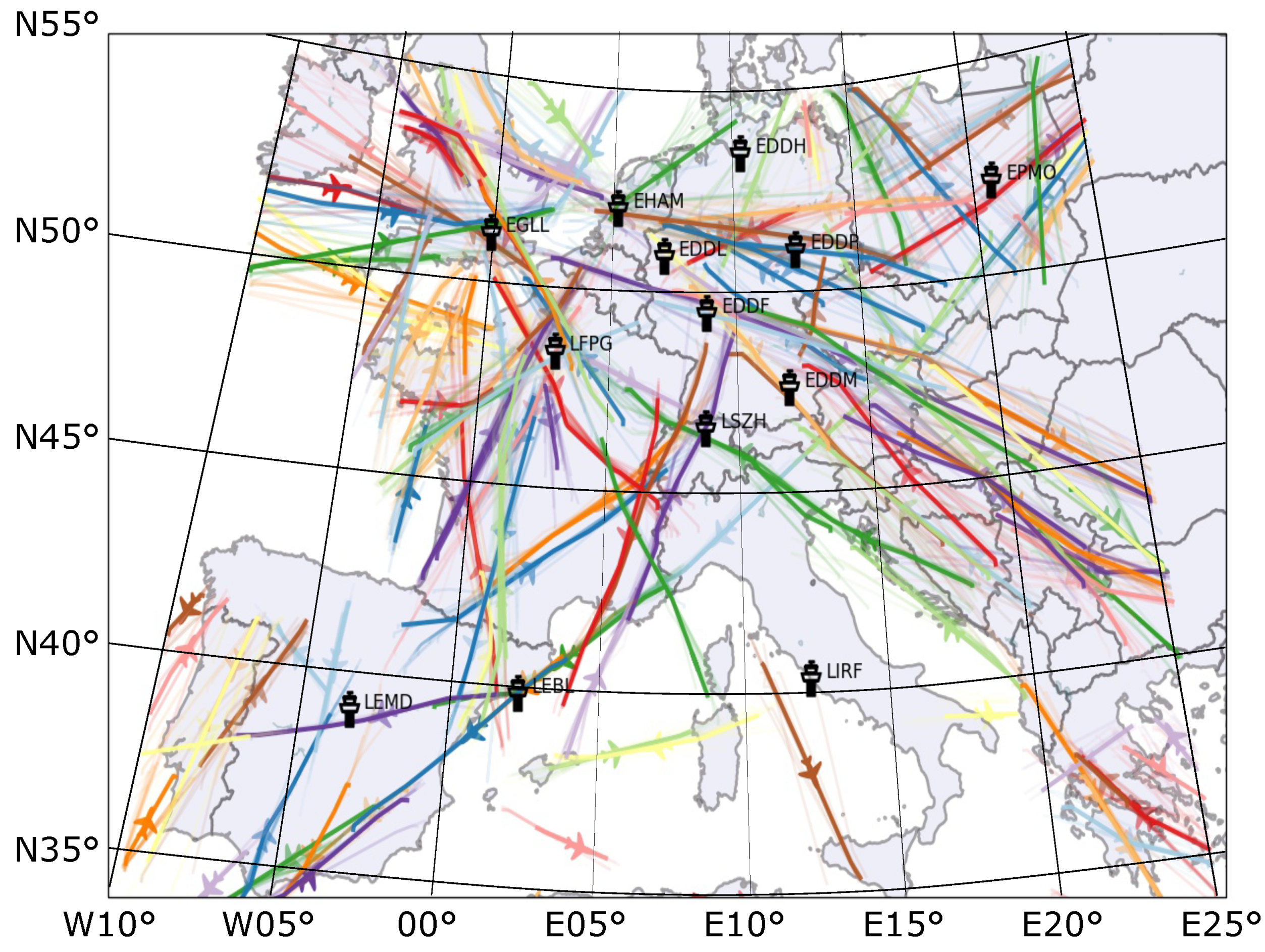
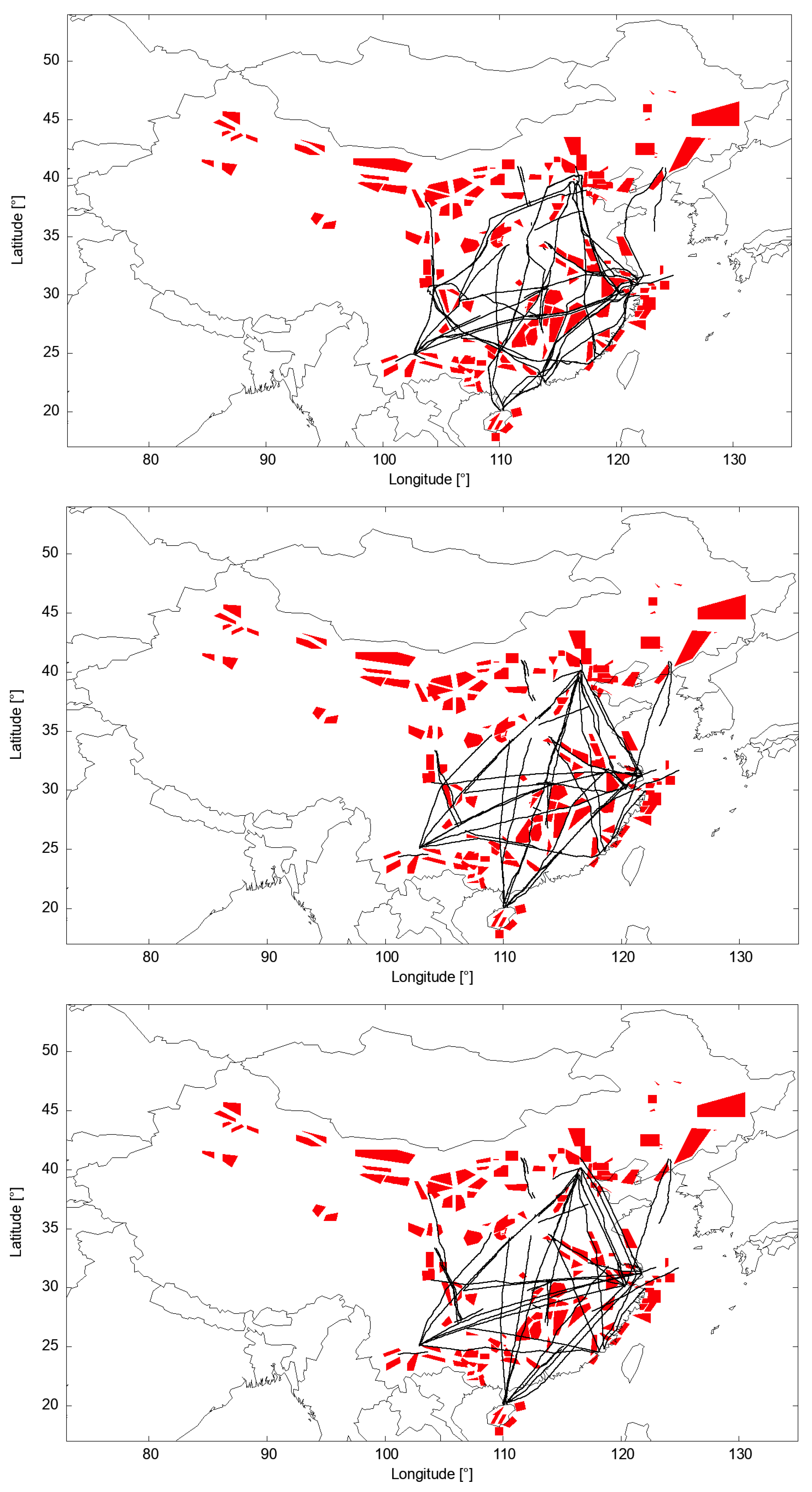
5. Chinese and European Representative Reference Trajectories

In the European data set, the final trajectory DBSCAN clustering using the parameters ε = 0.5 and M i n c = 10 forms 160 clusters. In total, 8670 of the 18,264 (i.e., 43%) trajectories has been assigned to clusters (as shown in Figure 5). For comparison, clustering the Chinese data set with the parameters ε = 0.5 and M i n c = 10 yields 99 clusters including 1653 of the 12,721 trajectories (i.e., 13%, see Figure 4).
Figure 4 and Figure 5 indicate clear differences in the distribution of air traffic within a similar area size, although a similar number of trajectories is considered. In Figure 4 and Figure 5 all trajectories belonging to a cluster are shown in the same colour in higher transparency as the reference trajectory. Compared to the European clusters, Chinese trajectories cluster more tightly around the reference trajectory and scatter less. Chinese air traffic appears to be limited to a few airways due to the high number of prohibited areas (176, see Figure 3).This seems to be the main reason for deviations from the great circle distance.
For a further comparison of the reference trajectories, the en-route horizontal flight efficiency (HFE) is compared between both continents. As a performance indicator for the route efficiency, HFE is the difference between the actual route flown and the shortest possible route, the great circle distance d GC [km]. Before calculating d GC , the trajectories are trimmed by the distance travelled in the TMA, approx. 40 NM around the airport reference point [65]. The HFE is used as a standard for data collection and processing under the responsibility of the Operations Unit in the Performance Review Unit’s (PRU) Department for Quality of Service Department and complies with IR317/2019. Both processes and procedures associated with the so-called HFE data flow are documented by the PRU’s quality management system. The indicator takes into account the en-route segments of flight f crossing an airspace (sector i) and compares the distance flown d flown , i , f with the achieved distance d achieved , i , f . Since this indicator focuses the horizontal efficiency, the achieved distance corresponds to the great circle distance d GC [65].
H F E i , f = d flown , i , f d achieved , i , f 1 · 100 %
Within a single sector, i, the distance flown d flown , i , f corresponds to the ground distance (in this study calculated from the ADS-B position data). The achieved distance d achieved , i , f is the difference between the great circle distance d GC from a sector entry point to the destination and the great circle distance from the sector exit point to the destination [65]. From this follows, the achieved distance d achieved , i , f depends on the fragmentation of the airspace, i.e., the number of sectors flown through. Furthermore, the achieved distance d achieved , i , f depends on the location of sector entry points and exit points. Giving a simple example by assuming a distance flown of d flown , i , f = 220 km within a sector i and an achieved distance of d achieved , i , f = 200 km , Equation (8) yields HFE = 10 % , i.e., the aircraft flew a 10 % diversions. The description ‘horizontal flight efficiency’ might be a bit misleading because following Equation (8) low values of HFE indicate a high efficiency [66,67].
However, since 2014, the Performance Review Report, published by Eurocontrol’s Performance Review Commission, publishes high values in Europe of HFE between 96.5 % HFE 98 % [37,68] indicating high efficiency. It seem, that the Performance Review Commission inverted dividend and divisor in Equation (8). Furthermore, ICAO discusses HFE as the efficiency with percentage values close to HFE = 100 % [69].
For example, in 2017, the worldwide HFE was between 92% and 94%, which corresponds to a deviation from d GC between 6% and 8%. In the Europe/North Atlantic region, the HFE reached 97.3 %, and in the Asia/Pacific region around 94% [69].
Nevertheless, this study strictly sticks with Eurocontrol’s definition of HFE in Equation (8) and calculates low values indicating high efficiency.
Although long flights usually approach d GC more closely than short distances [70] and in the observed Chinese flights have significantly longer distances, the deviation from d GC in Europe is an order of magnitude smaller than that in China (see Figure 6).
Ten of the 81 reference trajectories examined in the Chinese data set with a minimum distance of 200 km are below an HFE of 2%. For 48 Chinese trajectories, i.e., about 60% of the trajectories, the deviation was between 6 to 10%. Eight trajectories had an HFE of only 83 to 86%. On average, the HFE was 7.34 % or 84.7 km with an average route length of 1185 km (see Figure 7 for more details). The average route deviations of the Chinese reference trajectories, classified according to the length of the flight route is shown in Figure 6. Of the 81 trajectories examined, 55 were short-haul and 26 medium-haul flights. The lowest average deviation of 5.38 % is calculated for the extreme short-haul flights (flight distance 200 to 500 km), while short-haul flights with a flight distance of 1000 to 1500 km have the highest HFE of 9%.
In the European airspace, 147 of the 160 mean trajectories of the clusters (route length longer than 200 km) were investigated. 137 reference trajectories have an HFE of less than 2% (Figure 7). For 121 trajectories (82% of the trajectories), HFE is below 1%. The remaining six trajectories are assessed with an HFE between 2% and 6%. On average, European reference trajectories have an HFE of 0.67 % (see Table 2), corresponding to 3.5 km for an average route length of 508 km. 81 trajectories with a total distance between 200 and 500 km correspond to a mean HFE of 0.67 % (Figure 6). On average, HFE of 66 trajectories with a total distance between 500 and 1000 km was slightly higher with 0.69 %.

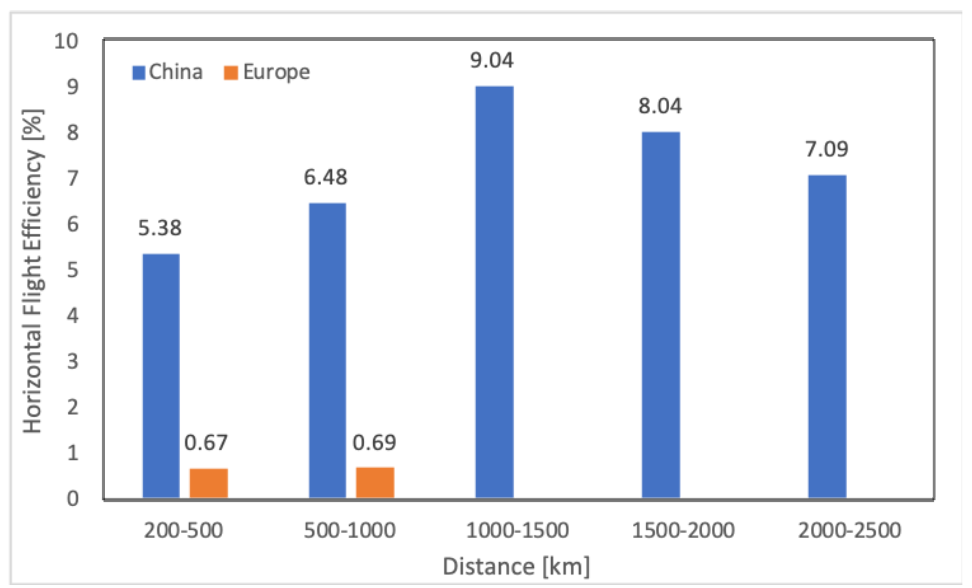
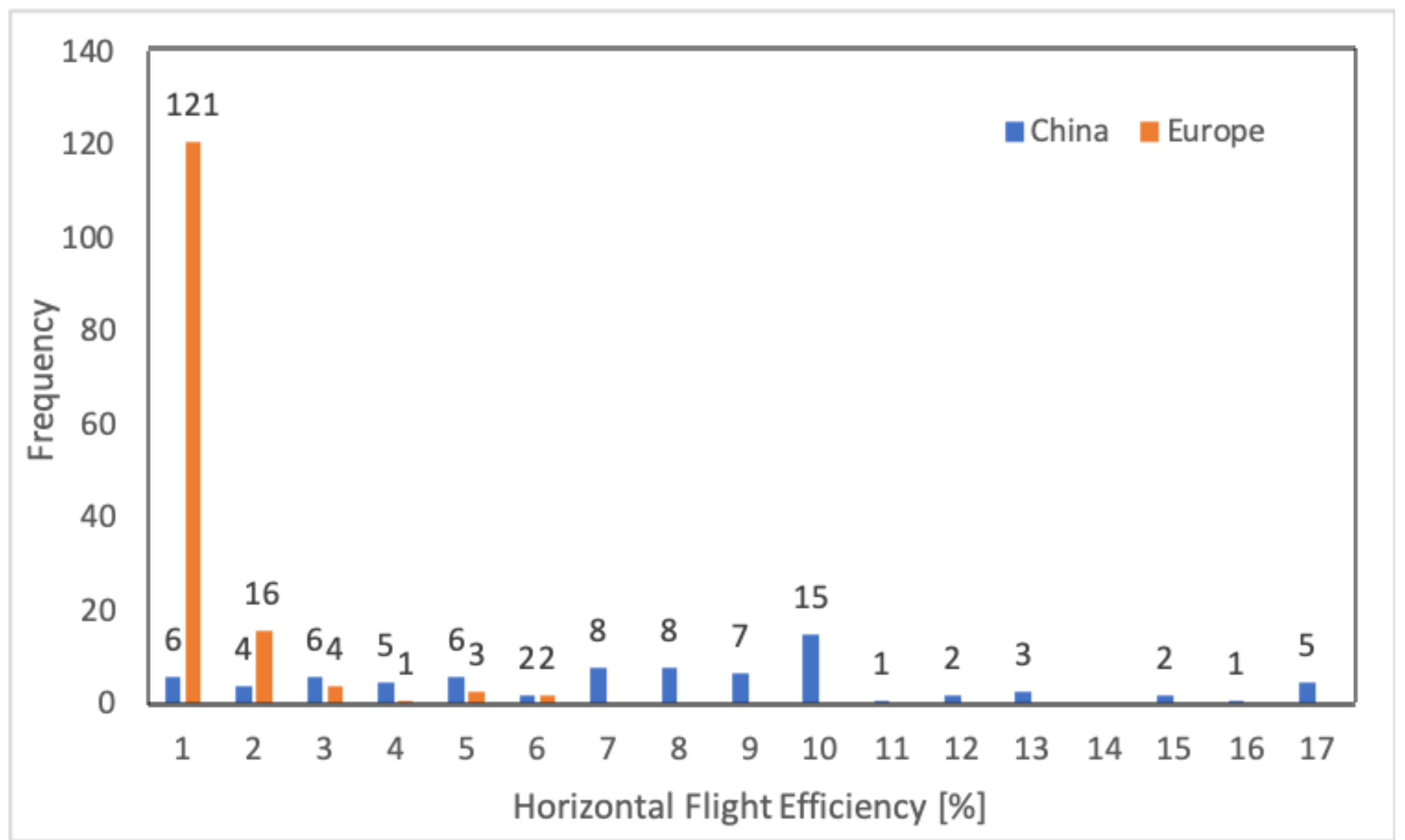
6. Differences between Real and Optimized Reference Trajectories

It is obvious that, compared to Europe, restricted areas in China have a greater influence on the efficiency of horizontal routing than local weather phenomena. This raises the question of whether Chinese air traffic can be made more efficient by taking the assumed restricted areas into account. For this purpose, the reference trajectories of both areas (China and Europe) were optimised concerning wind, overflight charges and restricted areas using an A-star pathfinding algorithm [62]. For the European data set, an airway structure (AIRAC Cycle) from April 2018 has been assumed as a grid structure. The comparison of the real and optimised flights is summarised in Table 3 and shown in Figure 8 and Figure 9. As expected, only 2.3 km per flight (maximum 52.84 km) could be saved on average in Europe. In China, on the other hand, the average was 255.81 km per flight (and a maximum of 890.33 km). To emphasise the influence of the restricted areas in China on the horizontal routing, the reference trajectories were additionally optimised without considering the restricted areas. With such operations, an average of 892.31 km per flight (and a maximum of 2485.06 km) could be saved in the study area. Furthermore, the HFE could be reduced to 2.08 % .
Unfortunately, the authors were not aware of the Chinese airspace structure (AIRAC cycle). For this reason, a freely selectable grid structure was provided to the path search algorithm in China, which probably does not correspond entirely to reality. By assuming free-route airspace, it is, therefore, possible that the optimised routes in China are not described by airways and waypoints.
As in any data analysis, internal and external uncertainties can neither be avoided nor clearly identified. From an external perspective, the publicly available data used may have been manipulated. For example, an unmentioned artificial enrichment of the data or an unfavourable handling of data gaps cannot be ruled out. However, the own data analysis showed gaps and false values to a reasonable extent and suggests that the data were not falsified. The test of correct implementation of data analysis in this study was purely graphical and convincing. Nevertheless, errors may have crept into the cluster algorithm despite already having several validated libraries, which remained undetected. The same applies to the simulation of the optimised trajectories. Finally, the comparison of historical and optimised trajectories was done manually. It follows that the results are carried out with the knowledge of different input data and political circumstances in China and Europe. This raises the possibility that the restricted areas in China have been given more importance than they deserve.
The rapid progress in data-based trajectory analysis implies the use of incorrect methods or parameter estimators. A different clustering method would probably have required more expert knowledge, such as the desired number of clusters or a weighting of the trajectory properties before clustering, which should be explicitly omitted in this study. For the sake of comparability, the same parameters were used for data sets in this study. It is possible that individually estimated parameters would have led to different reference trajectories and thus to different conclusions. However, the main influence on horizontal efficiency in China, blocked airspace, cannot be denied.

7. Conclusions and Outlook

In this study, operational constraints of the Chinese and European air traffic system and the optimization potential of horizontal routing in the upper airspace considering and neglecting the most important constraints have been analyzed and compared between two airspaces that are outwardly very similar (in terms of size, number of aircraft movements, number of airports, distances between airports as described in Section 2).
In both airspaces, representative trajectories were extracted based on historical flight movements using a DBSCAN cluster analysis, which were evaluated comparatively in detail. The diversions factor (described by the en-route HFE) and distance of the Chinese trajectories were on average an order of magnitude higher than in Europe. Already in the graphical representation of the reference trajectories (Figure 4 and Figure 5) the deviations from the great circle distance in China become apparent. The Chinese detours correlate very clearly with the presumed blocked airspaces, which due to their temporal volatility not only cause delays but also create inefficiencies in the horizontal routing. Nevertheless, the horizontal flight efficiency can be increased to 5.84 % despite assumed Chinese closed airspaces. It follows that provided the opening and closing times of the closed airspaces are known, the airspace structure design in China can certainly be improved. Both airspaces have similar basic meteorological conditions without significant weather-related disruptive factors at cruising altitude. This means that from a meteorological point of view, no particular restrictions are to be expected for cruising in China and Europe.
Since the flight planning and flight operation are recommended by ICAO [6] the procedures are very similar in both airspaces and do not suggest any significant differences in the routing. Since the representative trajectories of both airspaces and their main restrictions in cruise are known, further influencing factors on flight efficiency such as the choice of aircraft type, typical business models of the airlines and their handling of delays are to be examined comparatively in the future. The aim is always to examine the usability of publicly accessible flight tracks for increasing the efficiency of future air traffic.
The result of the cluster analysis has strong graphical similarities to other results of clustered trajectories. The graphical representations are comparable to results from [26,27,28,29,31,35,36]. From this, it follows that internal uncertainties are unlikely. Furthermore, the laterally optimized trajectories follow the great circle distance as close as possible. Since no strong winds occurred on the days of examination, the optimization results seem plausible.
In the future, as a logical consequence, vertical flight efficiency will be examined by optimizing the complete reference trajectories and comparing the vertical efficiency with the historic flights. Thereby, the aircraft mass and the airline business model must be estimated to correctly reflect local political and operational specificity. A further challenge in the analysis of vertical efficiency is the widely differing distances of the trajectories of the two datasets.

Author Contributions

Conceptualization: J.R.; methodology: J.R.; software: J.R., G.C., validation: J.R., G.C.; formal analysis: J.R.; investigation: J.R., resources: J.R., Y.W. data curation: J.R., Y.W.; writing—original draft preparation: J.R., writing—review and editing: J.R., H.F., Y.W.; visualization: J.R.; supervision: J.R., H.F., Y.W.; project administration: J.R.; funding acquisition: H.F., X.S., J.R. All authors have been read and agreed to the published version of the manuscript.

Funding

This work is financed by Deutsche Forschungsgemeinschaft (DFG, German Research Foundation) in the framework of the project UBIQUITOUS-410540389 and by the National Natural Science Foundation of China (Grant Nos.61861136005, 61851110763, and 71731001). This research received data from the National Natural Science Foundation of China (Grant Nos. U2033203 and U1833126).

Institutional Review Board Statement

Not applicable.

Informed Consent Statement

Not applicable.

Data Availability Statement

Not applicable.

Conflicts of Interest

The authors declare no conflict of interest.

References

  1. Civil Air Navigation Services Organisation. Implementing Air Traffic Flow Management and Collaborative Decision Making. Available online: https://canso.fra1.digitaloceanspaces.com/uploads/2020/02/Implementating-Air-Traffic-Fow-Management-and-Airport-Collaborative-Decision-Making.pdf (accessed on 3 January 2021).
  2. SESAR Joint Undertaking. European ATM Master Plan Edition 2; SESAR Joint Undertaking: Brussels, Belgium, 2015. [Google Scholar]
  3. European Commission. Regulation (EU) No 965/2012. Off. J. Eur. Communities 2012, L 296, 1–148. [Google Scholar]
  4. European Commission. Commission Implementing Regulation (EU) No 2019/123. Off. J. Eur. Union 2019, L 28, 1–49. [Google Scholar]
  5. International Civil Aviation Organization. Aeronautical Information Services (AIS) Aeronautical Information Regulation and Control (AIRAC); Annex 15; International Civil Aviation Organization: Montreal, QC, Canada, 2005. [Google Scholar]
  6. International Civil Aviation Organization. Procedures of Air Navigation Services, Air Traffic Management. Doc. 4444 PANS-ATM; International Civil Aviation Organization: Montreal, QC, Canada, 2016. [Google Scholar]
  7. European Commission. Flight Level Orientation Scheme—FLOS; Official Journal of the European Union: Brussels, Belgium, 2016. [Google Scholar]
  8. Whitley, A.; Park, K. China Air Traffic Congestion Worsened by Military Control. China’s Airlines Renew the Call for Airspace Reform. Bloomberg, 17 May 2013. [Google Scholar]
  9. European Defence Agency. The Military in the Single European Sky. Facts and Figures; European Defence Agency: Brussels, Belgium, 2018. [Google Scholar]
  10. Rosenow, J.; Förster, S.; Lindner, M.; Fricke, H. Multicriteria-Optimized Trajectories Impacting Today’s Air Traffic Density, Efficiency, and Environmental Compatibility. J. Air Transp. 2018, 27, 8–15. [Google Scholar] [CrossRef]
  11. Sun, J.; Hoekstra, J.M.; Ellerbroek, J. OpenAP: An Open-Source Aircraft Performance Model for Air Transportation Studies and Simulations. Aerospace 2020, 7, 104. [Google Scholar] [CrossRef]
  12. Everitt, B.; Landau, S.; Stahl, D.; Leese, M. Cluster Analysis; John Wiley & Sons: New York, NY, USA, 2011. [Google Scholar]
  13. Ester, M.; Sander, J. Knowledge Discovery in Databases—Techniken und Anwendungen; Springer: Berlin/Heidelberg, Germany, 2000. [Google Scholar]
  14. Driver, H.; Kroeber, A. Quantitative Expression of Cultural Relationships; University of California Publications in American Archaeology and Ethnology: Berkeley, CA, USA, 1932; pp. 211–256. [Google Scholar]
  15. Zubin, J. A technique for measuring like-mindedness. J. Abnorm. Soc. Psychol. 1938, 33, 508–516. [Google Scholar] [CrossRef]
  16. Tryon, R. Cluster Analysis; Correlation Profile and Orthometric (Factor) Analysis for the Isolation of Unities in Mind and Personality; Edwards Brother, Inc., Lithoprinters and Publishers: Ann Arbor, MI, USA, 1939. [Google Scholar]
  17. Cattell, R. The description of personality: Basic traits resolved into clusters. J. Abnorm. Soc. Psychol. 1943, 38, 476–506. [Google Scholar] [CrossRef]
  18. Olive, X. Traffic, a toolbox for processing and analysing air traffic data. J. Open Source Softw. 2019, 4, 1518. [Google Scholar] [CrossRef] [Green Version]
  19. MacQueen, J. Some methods for classification and analysis of multivariate observations. Berkeley Symp. Math. Stat. Probab. 1967, 5.1, 281–297. [Google Scholar]
  20. Dunn, J.C. A Fuzzy Relative of the ISODATA Process and Its Use in Detecting Compact Well-Separated Clusters. J. Cybern. 1973, 3, 32–57. [Google Scholar] [CrossRef]
  21. Defays, D. An efficient algorithm for a complete link method. Comput. J. 1977, 20, 364–366. [Google Scholar] [CrossRef] [Green Version]
  22. Ester, M.; Kriegel, H.; Sander, J.; Xu, X. A density-based algorithm for discovering clusters in large spatial databases with noise. In Proceedings of the Second International Conference on Knowledge Discovery and Data Mining (KDD-96), Portland, OR, USA, 2–4 August 1996; AAAI Press: Palo Alto, CA, USA, 1996; pp. 226–231. [Google Scholar]
  23. Ankerst, M.; Breunig, M.; Kriegel, H.; Sander, J. OPTICS: Ordering Points to Identify the Clustering Structure. In Proceedings of the ACM SIGMOD International Conference on Management of Data, Philadelphia, PA, USA, 31 May–3 June 1999; AAAI Press: Palo Alto, CA, USA, 1999; pp. 49–60. [Google Scholar]
  24. Xu, L.; Neufeld, J.; Larson, B.; Schuurmans, D. Maximum Margin Clustering. Adv. Neural Inf. Process. Syst. 2004, 17, 1537–1544. [Google Scholar]
  25. Li, L.; Das, S.; John Hansman, R.; Palacios, R.; Srivastava, A.N. Analysis of Flight Data Using Clustering Techniques for Detecting Abnormal Operations. J. Aerosp. Inf. Syst. 2015, 12, 587–598. [Google Scholar] [CrossRef] [Green Version]
  26. Campbell, A.; Zaal, P.; Schroeder, J.; Shah, S. Development of Possible Go-Around Criteria for Transport Aircraft. In Proceedings of the 2018 Aviation Technology, Integration, and Operations Conference, Atlanta, GA, USA, 25–29 June 2018. [Google Scholar]
  27. Sheridan, K.; Puranik, T.; Mangortey, E.; Pinon, O.; Kirby, M.; Mavris, D. An Application of DBSCAN Clustering for Flight Anomaly Detection during the Approach Phase. In Proceedings of the AIAA Scitech 2020 Forum, Orlando, FL, USA, 6–10 January 2020. [Google Scholar] [CrossRef]
  28. Verdonk, C.; Gomez Comendador, V.; Nieto, F.; García, M. Discussion On Density-Based Clustering Methods Applied for Automated Identification of Airspace Flows. In Proceedings of the 2018 IEEE/AIAA 37th Digital Avionics Systems Conference (DASC), London, UK, 23–27 September 2018; pp. 1–10. [Google Scholar] [CrossRef] [Green Version]
  29. Ling-Ling, B.; Yo-Beng, Z.; Chao, X. Application of Kernel DBSCAN Algorithm in Civil Aviation Customer Segmentation. Comput. Eng. 2012, 38, 70–73. [Google Scholar] [CrossRef]
  30. Lee, C.H.; Shin, H.S.; Tsourdos, A.; Skaf, Z. Anomaly detection of aircraft engine in FDR (flight data recorder) data. In Proceedings of the IET 3rd International Conference on Intelligent Signal Processing (ISP 2017), London, UK, 4–5 December 2017; pp. 1–6. [Google Scholar] [CrossRef] [Green Version]
  31. Chakrabarti, S.; Vela, A.E. Clustering Aircraft Trajectories According to Air Traffic Controllers’ Decisions. In Proceedings of the 2020 AIAA/IEEE 39th Digital Avionics Systems Conference (DASC), Virtual Conference, 11–15 October 2020; pp. 1–9. [Google Scholar] [CrossRef]
  32. Saez, R.; Khaledian, H.; Prats, X. Generation of emergency trajectories based on aircraft trajectory prediction. In Proceedings of the 2021 AIAA/IEEE 40th Digital Avionics Systems Conference (DASC), San Antonio, TX, USA, 28–30 September 2021; pp. 1–10. [Google Scholar]
  33. Olive, X.; Sun, J.; Murça, M.; Krauth, T. A Framework to Evaluate Aircraft Trajectory Generation Methods. In Proceedings of the 14th USA/Europe Air Traffic Management Research and Development Seminar, Saclay, France, 17–19 June 2021. [Google Scholar]
  34. Delahaye, D.; Puechmorel, S.; Alam, S.; Fero, E. Trajectory mathematical distance applied to airspace major flows extraction. In Proceedings of the 5th ENRI International Workshop on ATM/CNS, Nakano, Japan, 29–31 October 2017; pp. 51–66. [Google Scholar]
  35. Olive, X.; Morio, J. Trajectory Clustering of Air Traffic Flows around Airports. Aerosp. Sci. Technol. 2019, 84, 776–781. [Google Scholar] [CrossRef] [Green Version]
  36. Zeng, W.; Xu, Z.; Cai, Z.; Chu, X.; Lu, X. Aircraft Trajectory Clustering in Terminal Airspace Based on Deep Autoencoder and Gaussian Mixture Model. Aerospace 2021, 8, 266. [Google Scholar] [CrossRef]
  37. Performance Review Comission. Performance Review Report—An Assessment of Air Traffic Management in Europe during the Calender Year 2014, 2015, 2016; Eurocontrol: Brussels, Belgium, 2017. [Google Scholar]
  38. International Civil Aviation Organization. Second Meeting/Workshop of Air Traffic Management (ATM) Authorities and Planners; Working Paper, CAR/SAM/3 RAN Meeting Report; International Civil Aviation Organization: Montreal, QC, Canada, 2001. [Google Scholar]
  39. Civil Aviation Administration of China. China. 2020. Electronic Aeronautic Information Publication. Available online: http://www.eaipchina.cn/ (accessed on 28 March 2021).
  40. Civil Aviation Administration of China. Civil Aviation Law of the People’s Republic of China; Standing Committee of the National People’s Congress: Beijing, China, 2007. [Google Scholar]
  41. Yonggang, L. Flexible Use of Airspace in China. In Proceedings of the APAC Civil/Military Cooperation Lecture/Seminar, Beijing, China, 19–21 November 2014. [Google Scholar]
  42. Bergman, J. This Is Why China’s Airports Are a Nightmare. Available online: https://www.bbc.com/worklife/article/20160420-this-is-why-chinas-airports-are-a-nightmare (accessed on 25 March 2021).
  43. Eurocontrol. Free Route Airspace (FRA) Implementation Projections—2021. Available online: https://www.eurocontrol.int/publication/free-routeairspace-fra-implementation-projection-charts (accessed on 28 February 2021).
  44. Available online: http://www.eurocontrol.int/services/monthly-adjusted-unit-rates (accessed on 22 February 2021).
  45. Eurocontrol. Customer Guide to Charges; Central Route Charges Office: Brussels, Belgium, 2020. [Google Scholar]
  46. Spichtinger, P.; Gierens, K.M.; Read, W. Initial Information to EU, Other Member States and Other Interested Parties on the Establishment of FABEC; (EC) 550/2004 Service Provision Regulation as Amended by (EC) 1070/2009, Art. 9a 3. and 9a 4.; FABEC: Malchina, Italy, 2003. [Google Scholar]
  47. Ballesteros, J.A.; Hitchens, N.M. Meteorological Factors Affecting Airport Operations during the Winter Season in the Midwest. Weather Clim. Soc. 2018, 10, 307–322. [Google Scholar] [CrossRef]
  48. Gultepe, I.; Sharman, R.; Williams, P.D.; Zhou, B.; Ellrod, G.; Minnis, P.; Trier, S.; Griffin, S.; Yum, S.S.; Gharabaghi, B.; et al. A Review of High Impact Weather for Aviation Meteorology. Pure Appl. Geophys. 2019, 176, 1869–1921. [Google Scholar] [CrossRef]
  49. Shi, Y.; Song, L.; Xia, Z.; Lin, Y.; Myneni, R.B.; Choi, S.; Wang, L.; Ni, X.; Lao, C.; Yang, F. Mapping Annual Precipitation across Mainland China in the Period 2001–2010 from TRMM3B43 Product Using Spatial Downscaling Approach. Remote Sens. 2015, 7, 5849–5878. [Google Scholar] [CrossRef] [Green Version]
  50. Ueno, Y.; Hyodo, M.; Yang, T.; Katoh, S. Intensified East Asian winter monsoon during the last geomagnetic reversal transition. Sci. Rep. 2019, 9, 9389. [Google Scholar] [CrossRef] [PubMed]
  51. European Centre for Medium-Range Weather Forecasts. Forecasts. Available online: https://www.ecmwf.int/ (accessed on 25 March 2021).
  52. Tafferner, A.; Forster, C.; Hagen, M.; Hauf, T.; Lunnon, B.; Mirza, A.; Gouillou, Y.; Zinner, T. Improved thunderstorm weather information for pilots through ground and satellite based observing systems. In Proceedings of the 14th Conference on ARAM, 90th AMS Annual Meeting 2010, Atlanta, GA, USA, 17–21 January 2010; pp. 1–12. [Google Scholar]
  53. Gerz, T.; Forster, C.; Tafferner, A. Mitigating the Impact of Adverse Weather on Aviation. In Atmospheric Physics. Research Topics in Aerospace; Schumann, U., Ed.; Springer: Berlin/Heidelberg, Germany, 2012. [Google Scholar] [CrossRef]
  54. Taszarek, M.; Kendzierski, S.; Pilguj, N. Hazardous weather affecting European airports: Climatological estimates of situations with limited visibility, thunderstorm, low-level wind shear and snowfall from ERA5. Weather Clim. Extrem. 2020, 28, 100243. [Google Scholar] [CrossRef]
  55. Reiber, M. Moderne Flugmeteorologie für Ballonfahrer und Flieger: Die Theorie und ihre praktische Anwendung; Reiber; Antiquariat Fuchseck: Gammelshausen, Germany, 2002. [Google Scholar]
  56. Garcia, M.; Dolan, J.; Haber, B.; Hoag, A.; Diekelman, D. A Compilation of Measured ADS-B Performance Characteristics from Aiereon’s Orbit Test Program. In Proceedings of the 2018 Enhanced Solutions for Aircraft and Vehicle Surveillance (ESAVS) Applications Conference, Berlin, Germany, 18–19 October 2018. [Google Scholar]
  57. Rohde, R. Germany Trade and Invest—Gesellschaft für Außenwirtschaft und Standortmarketing mbH. Available online: https://www.gtai.de/gtaie/trade/branchen/branchenbericht/china/innerchinesischer-flugverkehr-und-tourismus-erholen-sich-569326 (accessed on 26 March 2021).
  58. European Commission. Commission Implementing Regulation (EU) No 1207/2011 of 22 November 2011 Laying down Requirements for the Performance and the Interoperability of Surveillance for the Single European Sky. Off. J. Eur. Union 2011, L 305, 35–52. [Google Scholar]
  59. Ali, B.S. Aircraft Surveillance Systems: Radar Limitations and the Advent of the Automatic Dependent Surveillance Broadcast; Routledge: London, UK; Taylor & Francis Group: New York, NY, USA, 2018. [Google Scholar]
  60. Kakubari, Y.; Kosuge, Y.; Koga, T. ADS-B Latency Estimation Technique for Surveillance Performance Assessment. In Air Traffic Management and Systems III. EIWAC 2017, Lecture Notes in Electrical Engineering; Electronic Navigation Research Institute, Ed.; Springer: Singapore, 2019; Volume 555. [Google Scholar]
  61. Douglas, D.; Peucker, T. Algorithms for the reduction of the number of points required to represent a line or its caricature. Can. Cartogr. 1973, 10, 112–122. [Google Scholar] [CrossRef] [Green Version]
  62. Förster, S.; Rosenow, J.; Lindner, M.; Fricke, H. A Toolchain for Optimizing Trajectories under Real Weather Conditions and Realistic Flight Performance; Greener Aviation: Brussels, Belgium, 2016. [Google Scholar]
  63. Rosenow, J.; Fricke, H.; Schultz, M. Air Traffic Simulation with 4D Multi-Criteria Optimized trajectories. In Proceedings of the 2017 Winter Simulation Conference, Las Vegas, NV, USA, 3–6 December 2017. [Google Scholar]
  64. Rosenow, J.; Michling, P.; Schultz, M.; Schönberger, J. Evaluation of Strategies to Reduce the Cost Impacts of Flight Delays on Total Network Costs. Aerospace 2020, 7, 165. [Google Scholar] [CrossRef]
  65. Eurocontrol Performance Review Unit. Eurocontrol Performance Review Unit. Performance Indicator—Horizontal Flight Efficiency. Available online: https://ansperformance.eu/methodology/horizontalflight-efficiency-pi/ (accessed on 12 February 2021).
  66. Standfuß, T.; Rosenow, J. Applicability of Current Complexity Metrics in ATM Performance Benchmarking and Potential Benefits of Considering Weather Conditions. In Proceedings of the Digital Avionics Systems Conference, San Antonio, TX, USA, 11–15 October 2020. [Google Scholar]
  67. Fricke, H.; Vogel, M.; Standfuß, T. Reducing Europe’s Aviation Impact on Climate Change using enriched Air traffic Forecasts and improved efficiency benchmarks. In Proceedings of the FABEC Research Workshop “Climate Change and Role of Air Traffic Control” 2021, Vilnius, Lithuania, 22–23 September 2021. [Google Scholar]
  68. Performance Review Comission. Performance Review Report 2019—An Assessment of Air Traffic Management in Europe during the Calendar Year 2019; Eurocontrol: Brussels, Belgium, 2020. [Google Scholar]
  69. Brain, D.; Voorbach, N. ICAO’s Global Horizontal Flight Efficiency Analysis; Environmental Report 2019 Chapter 4 Climate Change Mitigation: Technology and Operations; ICAO: Montreal, QC, USA, 2019; pp. 138–144. [Google Scholar]
  70. SES Single European Sky. SES Single European Sky. Commission Implementing Regulation (EU) 2019/317 of 11 February 2019 laying down a performance and charging scheme in the single European sky and repealing Implementing Regulations (EU) No 390/2013 and (EU) No 391/2013. Off. J. Eur. Union 2019, L 56, 1–67. [Google Scholar]
Figure 1. Assumed Unit Rates ( U R ) between 10.06 € (green) and 106.05 € (red) indicating overfly charges in Europe. Black polygons mark assumed restricted areas in Europe.
Aerospace 08 00338 g001
Figure 2. Method of clustering trajectories with DBSCAN and subsequent extraction of a reference trajectory per cluster. Trajectories are described by discrete data points. The core is a data point around which there are at least M i n c other points at a distance of ε . Here, ε is a distance measure considering track, latitude and longitude. Subsequently, the trajectory is chosen closest to all other trajectories within the cluster.
Aerospace 08 00338 g002
Figure 3. Assumed distribution and size of restricted Areas (black) in China. Restricted areas block 8% of the whole Chinese air space, but 70% of the eastern part, where the major air traffic takes place [42]. The color map indicates overfly charges of 1 € per kilometer (red) and 0.5 € per kilometer (yellow).
Aerospace 08 00338 g003
Figure 4. Reference Trajectories extracted in China after clustering the trajectories with ϵ = 0.5 and M i n c = 10 .
Aerospace 08 00338 g004
Figure 5. European reference trajectories extracted by clustering the trajectories with ϵ = 0.5 and M i n c = 10 . Each color represents a cluster. Trajectories belonging to a cluster are displayed with higher transparency than the reference trajectories.
Aerospace 08 00338 g005
Figure 6. Mean en-route Horizontal Flight Efficiency [%] (Equation (8)) of historic flight data in China (blue) and Europe (orange) depending on total ground distance. The Chinese data is taken from November 2020; the European data set is from May 2019.
Aerospace 08 00338 g006
Figure 7. Class-divided en-route Horizontal Flight Efficiency [%] (calculated with Equation (8)) of historic flight data in China (blue) and Europe (orange). The Chinese data is taken from November 2020, European data set belongs to May 2019.
Aerospace 08 00338 g007
Figure 8. Modeled (top) and optimized (middle) eastern Chinese reference trajectories (black) and assumed restricted areas (red). Considering restricted areas, air distances could be reduced by 48.988 km per flight on average, compared to the historical (modeled) scenario. (Bottom): optimized reference trajectories, ignoring restricted areas.
Aerospace 08 00338 g008
Figure 9. Modeled (top) and optimized (bottom) European reference trajectories (black) and assumed restricted areas (red). The European airspace seems to be dominated by direct connections. On average, only 2.33 km air distance could be saved per flight.
Aerospace 08 00338 g009
Table 1. Characteristics of the areas of investigation with relevance to trajectory clustering.
ChinaEurope
Coordinates
longitude [°][101–125][−10–25]
latitude [°][20–41][35–55]
Area size 9.6 × 10 6 km 2 10.5 × 10 6 km 2
Inhabitants 1.4 × 10 9 0.75 × 10 9
Mean number of movements per year 11.6 × 10 6 11.2 × 10 6
Number of investigated trajectories12,72118,264
parameters of DBCSAN
ε [a.u.] 0.5 0.5
M i n c [a.u.]1010
Number of clusters99160
Mean number of trajectories per cluster 16.4 54.2
Number of outliers87%53%
Table 2. Analysis of Chinese and European reference trajectories. Mean HFE corresponds to en-route HFE calculated with Equation (8).
ChinaEurope
Number of reference trajectories99160
Mean HFE [%] 7.34 0.67
Mean distance [km]1185508
Table 3. Benefit of optimized reference trajectories, compared to real trajectories in China and Europe. Mean HFE corresponds to en-route HFE calculated with Equation (8).
ChinaEurope
Number of reference trajectories99 160
Mean distance reduction [km]
considering restricted areas 255.81 2.33
ignoring restricted areas 892.31
Max. distance reduction [km]
considering restricted areas 890.33 52.84
ignoring restricted areas 2485.06
Mean HFE [%]
considering restricted areas 5.84 0.53
ignoring restricted areas 2.08
Publisher’s Note: MDPI stays neutral with regard to jurisdictional claims in published maps and institutional affiliations.

