
A Parametric Blade Design Method for High-Speed Axial Compressor


Institute for Aero Engine, Tsinghua University, Beijing 100084, China
Aerospace 2021, 8(9), 271; https://doi.org/10.3390/aerospace8090271
Submission received: 6 August 2021
/
Revised: 9 September 2021
/
Accepted: 13 September 2021
/
Published: 18 September 2021
(This article belongs to the Special Issue Fluid Flow Mechanics)
Abstract
:The blade geometry design method is an important tool to design high performance axial compressors, expected to have large design space while limiting the quantity of design variables to a suitable level for usability. However, the large design space tends to increase the quantity of the design variables. To solve this problem, this paper utilizes the normalization and subsection techniques to develop a geometry design method featuring flexibility and local adjustability with limited design variables for usability. Firstly, the blade geometry parameters are defined by using the normalization technique. Then, the normalized camber angle and thickness functions are proposed with subsection techniques used to improve the design flexibility. The setting of adjustable coefficients acquires the local adjustability of blade geometry. Considering the usability, most of the design parameters have clear, intuitive meanings to make the method easy to use. To test this developed geometry design method, it is applied in the design of a transonic, two flow-path axial fan component for an aero engine. Numerical simulations indicate that the designed transonic axial fan system achieves good efficiency above 0.90 for the entire main-flow characteristic and above 0.865 for the bypass flow characteristic, while possessing a sufficiently stable operation range. This indicates that the developed design method has a large design space for containing the good performance compressor blade of different inflow Mach numbers, which is a useful platform for axial-flow compressor blade design.
1. Introduction
Transonic axial-flow compressors are widely used in aero engines for the advantage of providing a high-pressure ratio per stage. High efficiency is one of the important targets for transonic axial compressors since it is beneficial for improving the engine’s fuel efficiency and leads to lower fuel costs and longer flight range [1]. Among the influencing factors, the blades’ design is an important factor having significant influence on the efficiency of transonic axial compressors [2,3,4]. In the design procedure of the transonic compressor, the blade is designed by using a geometry design method with related aerodynamic design criteria or combined with an optimization algorithm. Therefore, a flexible and practical geometry design method, having sufficient design space to contain the blade shape with excellent aerodynamic performance, is useful to improve the efficiency of transonic compressors.
The modern transonic compressor blade consists of several two-dimensional blade elements, referred as the airfoils, along the radial stacking line. The airfoil geometry has important influence on the aerodynamic performance of the compressor blade by affecting the S1 stream-surface flow. The Double Circular Arc airfoil (DCA) and the further developed Multi Circular Arc airfoil (MCA) are the most widely used airfoils in the early stage design of transonic axial compressors [5]. The MCA has improved design flexibility compared with DCA by combining several circular arcs of different curvature radius, forming the airfoil surfaces to alter the deflection for better controlling the shock strength, which achieves higher efficiency for Mach numbers larger than . In 1972, Wennerstrom et al. proposed a series of camber-line and thickness distribution functions incorporating adjustable coefficients for design flexibility for high Mach number compressor airfoils design [6]. The selection of the adjustable coefficient value in the functions depends on the design experiences. These design functions were applied in the transonic axial compressor [7,8] and achieved a stage isentropic efficiency of 0.882 with a pressure ratio of 2.065 [9]. In 1993, Korakianitis et al. [10] proposed a prescribed surface curvature distribution blade design method (CIRCLE) for designing turbo-machinery airfoils and blade. This method is based on the fact that the surface curvature has significant influence on local velocity (especially in the subsonic flow). Therefore, selecting the surface curvature as the design variable is beneficial for accurately obtaining the optimized flow. In 2007, Kulfan presented a universal parametric geometry representation method, referred to as CST [11,12]. By introducing the class function and shape function transformation techniques, this method can efficiently create different wing-airfoil-type shapes for aviation by varying several geometric variables. In 2017, Denton proposed a blade shape design method by inputting a table of camber-line angle and thickness against a fraction of meridional chord. Several control points are used to vary the camber-line angle linearly between the input points. The blade thickness shape could be varied by three design variables.
Besides, experimental and numerical investigations on flow mechanism of transonic compressor and airfoils provided useful information for the blade aerodynamic design. In the aspect of transonic airfoils, in 1984, Schreiber et al. systematically investigated the influence of inlet Mach number (from 0.8 to 1.1) and stream-tube contraction on the surface Mach number distribution, shock structure and loss coefficient level of a transonic airfoil [13]. In 2009, Sonoda and Olhofer et al. optimized the supersonic airfoil PAV-1.5 by using the evolutionary algorithm (ES) and obtained 24% reduction of total pressure loss coefficient due to the entropy reduction in the region around the suction surface by optimizing shock structure [14]. In 2016, Venturelli and Benini conducted a multi-objective design optimization on the PAV-1.5 based on the Kriging-assisted evolutionary algorithm, which obtained 25% reduction of loss coefficient and 6.5% increase of static pressure ratio due to decrease in the pre-shock Mach number by increasing the pre-compression strength [15]. In the aspect of transonic compressor, in 1993, the investigation by Wadia et al. on a high through-flow, low aspect ratio rotor indicates that the maximum thickness location can influence the shock loss level by changing the leading edge wedge angle and the optimum maximum thickness location for this rotor is between 55% and 60% chord location [2]. In 1996, Wadia et al. researched the effect of cascade area ratios on the transonic compressor performance [3]. A lower throat margin results in increased high-speed efficiency due to the reduction of shock loss and a slightly improved stall line but a lower part-speed performance. Reducing the trailing edge effective camber leads to the peak efficiency level improvement without significantly lowering the stall line. In 2004, Oyama et al. optimized the Rotor 67 by using evolutionary algorithms and increased the adiabatic efficiency by 2% because of the reduction of radial length and strength of the passage shock wave [16]. In 2010, Wang et al. proposed an adjoint aerodynamic design optimization method for blades in multistage turbomachines and the redesign of Rotor 67 by this method leads to remarkable isentropic efficiency increase because of weakened shock strength [17,18]. Another important research aspect is the optimizations of the three-dimensional sweep and bow to improve the blade aerodynamic performance [19,20]. In 2015, the numerical investigation by Ilikan et al. on an axial fan indicated that the sweep is able to influence the inflow axial velocity distribution and therefore affects the incidence and thus the aerodynamic load distribution of the blade [21]. In 2021, Richard et al. conducted multidisciplinary design optimization to improve the aerodynamic performance of an electric-ducted fan rotor using free-form deformation (FFD) and data mining techniques [22]. Data mining indicates that the key design variable blade twist, sweep, chord and hub thickness distribution had the most influence for the efficiency improvement of the optimized rotor.
Recently, the design of the compressor and fan blades has reached the custom design level, which requires that the geometry design method should be able to optimize the blade shape at a more detailed level to acquire the desired flow field [23]. Therefore, this paper is devoted to proposing a parametric blade geometry design method which can satisfy the custom design of the high performance compressor blade. To utilize the research findings on blade geometry, in the method developed in this paper, the key blade parameters (inlet and outlet metal angle , maximum thickness location , chord c, LE and TE relative thickness and shape, etc.) are specified by the designers, which is beneficial for rapidly establishing a good blade geometry. To ensure the quality of this compressor blade design method, compared with previous blade geometry design methods, the method developed in this paper is devoted to advancing the following aspects:
- 1.
- Flexibility
- 2.
- Local adjustability
- -
- Partial blade surface could be altered according to design needs while other parts of the airfoil are kept fixed, which is useful in blade optimizations.
- 3.
- Usability
- -
- The quantity of parameters is limited to a suitable level to make the method easy to use.
- -
- The parameters have clear, intuitive effects on the blade geometry [24].
In this paper, the blade geometry parameter is defined by using the normalization technique. Then, the subsection technique is used to establish the camber angle and thickness distributions for ensuring sufficient design flexibility and local adjustability. Next, the procedure from airfoils to three-dimensional blade and the definition of sweep and bow are elaborated. To test this developed geometry design method, it is applied in the design of a transonic, two flow-path axial fan component for an aero engine. Numerical simulations indicate that the designed transonic axial fan system achieves good efficiency above 0.90 for the entire main-flow characteristic and above 0.865 for the bypass flow characteristic while possessing a sufficient stable operation range, which indicates that the developed design method is a practical platform for axial-flow compressor blade design.
2. Two-Dimensional Blade Airfoil Design
2.1. Airfoil Definition
The design flexibility could be the most important feature to acquire the capability to design high performance compressor airfoils. Higher design flexibility tends to require more adjustable coefficients. However, in view of the usability, the quantity of the adjustable coefficients should be limited to a suitable level to make the method easy to use. To solve this problem, the normalization technique and subsection technique will be used.
The airfoil surfaces are obtained by stacking the relative thickness distribution in the normal direction of the camber-line, as shown in Figure 1. In this method, the camber angle distribution is specified to create the airfoil rather than the camber-line for two reasons. First, the airfoil surface slope has an important influence on supersonic flow [3,24] and it is more intuitive to tune the camber angle distribution to change the surface angle for obtaining the desired surface velocity distribution and shock structure [3]. Second, since the camber angle distribution is defined as the angle between the x-direction and the tangential line of the camber-line at each point from , which is equivalent to the slope of the camber-line. Therefore, by using camber angle distribution , less inner boundary conditions at the junction point need to be accommodated to ensure the curvature of camber-line continuity. To eliminate the scale effect of cascade parameters on creation functions, the normalized camber angle distribution is defined as:
The term θ in Equation (1) is the camber angle of airfoil which is known (given by the designer) when an airfoil will be generated. For the compressor blade, the camber angle θ of each airfoil can be calculated from the inlet and outlet metal angle (according to the through-flow calculation result):
Besides, the camber angle θ is equal to according to the definition of camber angle distribution . Then, the camber-line can be determined by integrating:
Since the terminal point of the camber-line is on the chord, once the normalized camber angle distribution is ascertained, the LE construction angle can be ascertained by solving 0 with several iterative calculations.
The function represents the relative thickness distribution, which is the diameter of the inscribed circle of the airfoil surface along the chord-wise direction. Similarly, the normalized thickness distribution is defined:
The boundary conditions for normalized thickness distribution are:
The parameter is the chord-wise location of maximum thickness. According to the airfoil definition, the un-staggered airfoil surfaces can be determined with ascertained distributions of and :
If the inlet metal angle is specified, the airfoil stagger angle can be determined:
Then, by rotating about the origin point (0, 0), the coordinates of staggered airfoil surfaces with specified chord C can be determined (Figure 2):
Therefore, in this design method, the main part of an airfoil can be created by specifying the aerodynamic chord , camber angle , maximum relative thickness , LE and TE relative thickness , normalized camber angle distribution and thickness distribution . With the geometry information provided by the generated main part of the airfoil, the LE and TE can be generated according to the required form. Since the cascade parameters () are usually determined according to through-flow calculation, the flexibility and usability of the method mainly rely on the functions and . The verified functions for and , which have been proved practical in compressor airfoil and blade design, are proposed in the next section.
2.2. Normalized Camber Angle Distribution
The flexibility and local adjustability of normalized camber angle distribution are achieved by using the subsection technique with carefully specified adjustable coefficients. According to the airfoil geometric features, the normalized camber angle distribution is designed as a segmented function combination of sub-functions and (Figure 3):
To find a suitable function for and in Equation (11), the normalized camber angle distribution of many high performance super/transonic compressor airfoils are extracted and summarized. After testing different functions, it is found that the normalized camber angle distribution in Equation (11) with sub-functions in Equation (12) and in Equation (13) can lead to good fitting results by tuning the adjustable coefficients while satisfying the boundary conditions (Figure 3a). The first segment function is for the inlet portion of an airfoil, which starts from the leading edge to the cascade passage inlet location. The inlet segment has an important influence on the strength of the cascade shock system as well as the magnitude of shock loss [25,26]. The second segment function affects the flow in the cascade passage [3] and provides the flow diffusion for pressure rise downstream the shock system, which starts from the passage inlet location to the trailing edge. As shown in Figure 3a, the is a strength coefficient determining the ratio of the camber-line deflection angle of the first segment to the overall camber angle. According to the boundary condition of function , the strength coefficient of the second segment is . is the location coefficient determining the termination of the first segment. For transonic airfoil, the inflection point of camber-line can be conveniently and accurately specified by using the location coefficient . The terms in sub-functions and deciding the first derivative at junction point are correlated and therefore the first derivative of function is ensured to be continuous. By altering the coefficients and , a wide range of normalized camber angle distribution can be created (Figure 3b). As described later, the corresponding shock structure and flow diffusion in the rear portion of the created airfoil will significantly change.
To acquire local adjustability, the sub-functions and are designed to have several adjustable coefficients (Equations (12) and (13)). As shown in Figure 4a–d, the coefficient determines the shape of the first segment and influences the inlet portion surface angle as well as the passage throat width. The coefficient determines the slope of the at location to provide a smooth transition. The second segment has three adjustable coefficients for providing a large design space to contain the suitable distribution in cases of different Mach number, solidity and camber angle. The effective region for , and in the second segment are front, middle and rear. The coefficients mainly affects the blade passage width at inlet and outlet as well as the variation gradient (Figure 4e–h), which can be used to adjust the flow diffusion rate after the inlet shock.
In general, the localized adjustable coefficients and allow to alter the specific part of the airfoil in detail level while keeping other parts fixed, which is useful for optimizing compressor airfoils. Table 1 summarizes the input parameters of normalized camber angle distribution .
2.3. Normalized Thickness Distribution
The normalized thickness distribution is also supposed to have sufficient design flexibility with good usability. An effective way to achieve these objectives is to use the subsection design technique, namely, describing the normalized thickness distribution with two equations (Figure 5a): One from the leading edge to the maximum thickness location and the other from that to the trailing edge:
The maximum thickness chord-wise location is a natural selection as the joint point of and since the value and slope of at location are fixed and suitable to be taken as the boundary conditions. To keep the curvature of continuous at the junction point, the following boundary conditions need to be satisfied:
To acquire the local adjustability, the slope of at the leading edge and the trailing edge, represented by the coefficients and , respectively, are expected to be specified by designers:
With the specified coefficient , the airfoil LE wedge angle can be determined:
The curvature (equivalent to the second order derivative since is 0) of at the maximum thickness location , represented by the coefficient , is also expected to be specified by designers:
According to these requirements, after testing different functions, it is found that the fourth order polynomials in Equations (22) and (23) are suitable for establishing the sub-functions and :
By applying the boundary condition Equations (5) and (15)–(20) to the basic form of the fourth order polynomials (Equations (21) and (22)), the unknown coefficients ( and ) can be ascertained (derivations in Appendix A). With the determined coefficients ( and ), the sub-functions and can be determined:
In this frame, by changing the maximum thickness location and adjustable coefficients , a wide range of which are suitable for airfoils of different inflow Mach numbers can be generated (Figure 5b). The adjustable coefficients , and allow user to alter the corresponding region of in detail level while keeping other part fixed. Figure 6 shows the effect of coefficients on thickness distribution, blade airfoil shape, surface angle and blade passage width distribution, which can be used to guide the selection of for better aerodynamic performance. Since the influence of coefficients are proportional to the maximum relative thickness , therefore, in supersonic airfoils, the camber-line has dominant influence on the airfoil shape. But in subsonic airfoils with higher thickness, the influence of thickness distribution on blade geometry is increased. Table 2 shows the input parameters of normalized thickness distribution .
3. From Airfoils to Three-Dimensional Blade Design
Stacking of Blade Element
Figure 7 shows the schematic for procedure from airfoils to three-dimensional blade. This procedure is able to transform the two-dimensional airfoil to an arbitrary projection revolution surface and a paper has been published to illustrate the details of this procedure [27]. An LE and TE creation module is incorporated and it can provide circular, elliptic (semiaxis ratio is specified by designer) and curvature-continuous LE and circular TE. The three-dimensional blade is obtained by stacking airfoils according to the center of gravity. The projection revolution surface for each blade element is ascertained by interpolating the hub and shroud surface according to the relative span height of LE and TE :
As mentioned previously, the blade aerodynamic performance can be effectively improved by proper sweep and bow [21,28,29,30]; therefore, the center of gravity of blade airfoils is allowed to be moved for acquiring the desired three-dimensional sweep and bow in two modes (Figure 7): Mode 1—move the centers of gravity along the axial and tangential directions; and Mode 2—along the stagger angle of the airfoil and its normal direction. In both modes, the move distances are given by the users in the input file of this developed blade design system.
4. Numerical Simulation Method Verification
To test this developed geometry design method, it is applied in the design of a transonic, two flow-path axial fan component for aero engine. Considering that the numerical simulation is used in the design for determination of flow field and aerodynamic performance, the transonic, high performance rotor, Rotor 67 (Figure 8), is used to verify the numerical simulation method since extensive experimental results of Rotor 67 are available in published literatures [31,32].
The numerical simulations are based on the steady Reynolds-averaged Navier–Stokes method (RANS) and conducted by the commercial CFD software Numeca. The central difference scheme and Spalart–Allmaras (SA) turbulence model are used. For boundary conditions, the inlet flow is set to uniform and pure axial with property of 288.15 K and 101,325 Pa. The static pressure is imposed at the center location with radial equilibrium chosen for outlet. The outlet static pressure is gradually increased to improve the rotor pressure ratio. The static pressure profile at the outlet is found by the radial equilibrium.
In this verification, the mesh for simulations has a multi-block structure with one O-block around the profile and four H-blocks. The wall cell height is set to 0.005 mm to yield an average value of and the wall cell height expansion ratio is set to 1.10 for sufficient grid density near the blade surface. The blade tip clearance is set to 1.0 mm according to the experiment.
To determine the proper mesh size, a grid independency study is conducted (Table 3). As shown in Figure 9a, the performance at the near stall point is more sensitive to the mesh size. Once the mesh density reaches the level of Grid 3, the variation of converged mass-flow and adiabatic efficiency become very small, which indicates that the grid independency has been reached in this case. As shown by Figure 9b, the calculated efficiency and total pressure ratio of Grid 4 show the same trend as the experimental data [32] but slightly lower in values, especially in the near stall range. An analysis of the flow field indicates that the slight difference at the near stall point is mainly caused by the shock-wave shape captured by numerical calculation, which is different compared to the experimental results (Figure 10). In general, this numerical method can predict the efficiency and total pressure ratio with good accuracy and important phenomena like the leading bow shock and passage shock captured by this method are also close to the experimental results [32].
5. Application Case: Efficient Transonic Axial Fan Design
5.1. Introduction of the Transonic Axial Fan System
The application design case for testing the developed geometry design method is a transonic, two flow-path axial fan component for aero engine with the objective of achieving high efficiency in the frequently used operation range. The transonic axial fan system has an overall inlet mass flow rate of 29.0 kg/s and a bypass ratio of 2.0 at the design point. The transonic axial fan is designed to deliver a stagnation pressure ratio of 2.8 at the main-flow outlet and 1.7 at the bypass outlet. The meridian view of this transonic axial fan system is shown in Figure 11.
The three-dimensional simulations of this axial fan component are conducted by the commercial CFD software Numeca with the steady Reynolds-averaged Navier–Stokes method (RANS) used. For the setup, the central difference scheme and Spalart–Allmaras (SA) turbulence model are used. The mesh for simulation has an O4H topology around each blade. The wall cell height is set to 0.002 mm and the expansion ratio is set to 1.15. The O-block around each blade has 25 pitch-wise nodes across the block for capturing the blade surface boundary-layer development. The number of stream-wise nodes and radial nodes of each blade surface is in the range from 57 to 101 and 57 to 105, respectively. The overall mesh has nodes.
5.2. Blade Design
In the design of a compressor system with given mass flow and total pressure ratio, the first step could be the selection of one-dimensional design parameters (the load coefficient and the flow coefficient ) for each stage to obtain good efficiency potential. For typical axial compressors, this can be achieved by referring to the Smith chart [33,34]. The final used load coefficient and flow coefficient of each stage are given in Table 4. The load coefficients of stages 1 to 3 are all above 0.30, which is a relatively high level.
With the numerical simulation to obtain the flow field, by using the developed parametric design method, the blade design for each stage mainly consists of two related parts: (1) Design of blade parameter radial distribution and (2) design of normalized camber angle and thickness distributions of blade elements. To elaborate this, the specific design procedure of Rotor 1 is represented in this section.
The inlet Mach number is one of the most important parameters influencing the blade design by affecting the selection of the incidence angle, relative thickness and normalized camber angle and thickness distributions. Figure 12a shows the inlet Mach number of each blade at the design point. It can be found that the Rotor 1 has a relative inlet Mach number from 0.6 at root and 1.3 at tip. Therefore, the design of Rotor 1 has to use all the airfoil types: Subsonic airfoils () at the root part (R = 0–0.30), transonic airfoils () at the mid part (R = 0.30–0.85) and S-type airfoils at the tip part (R = 0.85–1.0). In the first design part of Rotor 1, the inlet metal angle is finally designed to obtain an incidence angle from 5.5 degrees at root and gradually decreasing to 3.3 degrees around blade tip (Figure 13a). The corresponding suction surface incidence is −5.0 degrees at root, varying to 0.3 degrees at R = 0.2 and finally reaching 1.5 degrees around the blade tip. The calculated surface Mach number distributions (Figure 14) indicate that the above selection of incidence leads to a suitable front loading level, no flow blockage in the blade tunnel or excessive flow deceleration appearing on the front portion of the suction surface before the shock impinging point. The outlet metal angle and the solidity (by specifying the chord c) are co-designed to achieve the anticipated radial distribution of the rotor total pressure ratio (Figure 15a) while keeping the diffusion factor DF at a suitable level. The diffusion factor DF presented by Lieblein [35] is used to evaluate the aerodynamic loading level of the blade sections. The calculated diffusion factor DF of designed Rotor 1 is in the range of from 0.45 to 0.50 at most span (Figure 15b), which is at the proper level for the design point and has a sufficient margin to stall level ().
For the blade thickness, the selection of maximum thickness and its chord-wise location are mainly based on the inlet Mach number with the objective of obtaining a suitable blade loading distribution or shock structure while providing sufficient strength reservation for blade structure integrity. As shown in Figure 13b, Rotor 1 is designed to have a maximum thickness of 9.6% at the root and gradually decreases to 4.3% at the mid and finally to 2.5% at the tip. The ratio of LE thickness to maximum thickness is designed in the range of from 0.18 to 0.25, which is a balance between the leading edge bow shock loss and the structure strength of the LE portion. The maximum thickness location is designed to be 0.40 at the blade root for subsonic airfoil and increases approximately linearly to 0.65 at the blade tip for supersonic airfoil (Figure 13c).
The second part of the blade design is the designing of normalized camber angle and thickness distributions with the objective of achieving high efficiency. For the hub part (R = 0–0.30) of Rotor 1, the inlet relative Mach number is from 0.6 to 0.8, which belongs to the typical range of subsonic airfoils (). Therefore, a front-loading type normalized camber angle is used for this part (Figure 13d, R = 0) to obtain a uniform, shock-free loading distribution along the blade (Figure 13d). To achieve this, the selection of strength coefficient and the maximum thickness location are co-designed to control the flow acceleration on the former suction surface for keeping a suitable peak Mach number and to obtain a shock-free deceleration around the peak for low loss coefficient. As shown in Figure 14a, the surface Mach number of blade section at R = 0.1 has a suction surface peak Mach number of 0.92 at with a linear deceleration to the trailing edge without boundary-layer separation.
For the mid part of Rotor 1 (R = 0.30–0.85), the inlet relative Mach number is from 0.8 to 1.25, which belongs to the transonic airfoils. To control the strength of flow acceleration along the suction surface, a small, positive value of camber angle turning is used in this part (Figure 13d). To match the first segment of camber angle distribution with the inlet portion of airfoil, the location coefficient is specified near the shock impinging point on the suction surface (Figure 13d). The first segment of normalized thickness distribution is designed to have a small value of of 2.41 to 2.30 (Figure 13f) with an intermediate maximum thickness of 5.2% to 3.2% for the mid part (R = 0.3–0.85) to keep a small LE wedge angle for decreasing LE bow shock strength. With the above design, the first segment of normalized camber angle distribution (Figure 13e) and the maximum thickness location are co-designed to obtain a moderate pre-shock Mach number between 1.1 and 1.3 (Figure 14b–d), which can utilize the pressure rise at very low cost of total pressure loss. The design of the second segment of and the selection of and of aim at obtaining a continuous, separation-free deceleration after the suction surface shock impinging point to the trailing edge (Figure 14b–d)) for low boundary-layer growth (i.e., low viscous loss).
For the tip region of Rotor 1 with an inlet relative Mach number above 1.25, a negative value of camber angle turning is used in the tip region (R = 0.85–1.0) to generate an “S” shaped camber-line with concave surface inlet portion (Figure 13d–f), aiming at reducing the pre-shock for reducing the shock losses and related viscous losses for high efficiency. For the Rotor 1 tip part (R = 0.85–1.0), the location coefficient is specified at approximately 5% chord ahead of the peak Mach number location to provide a sufficient blade passage throat area for rotor performance at partial speed (Figure 13d). The first segment of normalized thickness distribution is designed to have a lower value of of 2.30 with small maximum thickness of 2.8% to 2.5% for the tip part (R = 0.85–1.0) to keep a small LE wedge angle for decreasing LE bow shock strength. The design of the second segment of and the selection of and of aim at obtaining a proper flow deceleration rate (in other words, surface pressure gradient) after the suction surface shock impinging point to prevent boundary-layer separation for low viscous loss (Figure 14e). In the design, the information of the shock impinging point on suction surface and the blade surface Mach number distribution are obtained from the simulation result; therefore, the design starts with a preliminary selection of input design parameters, (i) blade radial distribution of cascade parameters c, T, , etc., and (ii) design coefficients of and ) based on existing design cases of axial fan or compressors and continuing with iterations to optimize the input design parameters based on the analysis of simulation of the designed axial fan.
With the above design of Rotor 1, the numerical simulation indicates that Rotor 1 achieves a high adiabatic efficiency of 0.948 at the design point with the required total pressure ratio obtained. From the efficiency profile in Figure 15c, the adiabatic efficiency of Rotor 1 is above 0.950 at most locations, which indicates the rationality of the blade design.
To elaborate the design of stators, the design details concerning Stator 2 are represented here. As mentioned previously, the inlet Mach number has significant influence on the blade design and Stator 2 has a Mach number around 0.6 from root to tip (Figure 12a), which is in the typical subsonic range. Therefore, the subsonic airfoil is applied for this blade with the objective of low loss coefficient and wide operation range.
The inlet metal angle of Stator 2 is designed to obtain an incidence angle from 0 degrees at root and decreases to -2.4 degrees around tip at design point (Figure 16a). A lower incidence is used in the tip region (R = 0.80–0.95) of Stator 2 which can reduce the incidence level at decreased inlet mass flow and is beneficial for obtaining a low-loss level at off-design conditions. The outlet metal angle is specified to provide the anticipated pre-swirl for acquiring a suitable inflow angle of downstream rotor. The solidity is specified to 1.49 at the root and linearly increases to 1.28 at tip (Figure 16b). The corresponding diffusion factor DF is 0.5 at the root, decreasing towards tip and keeps below 0.45 at most of the span (Figure 18a), which is a reasonable level for the stator blade. For blade thickness, Stator 2 is designed to have a maximum thickness of 6.0% at the root and linearly increases to 6.5% at the tip (Figure 16c). The ratio of LE thickness to maximum thickness is designed to be 0.20 for the overall blade, which can obtain a small leading edge spike height (for low viscous loss) while satisfying the structure strength demand for LE.
In the second design part of Stator 2, a moderate front-loading type normalized camber angle distribution is used for this subsonic blade (Figure 16d) to obtain a continuous acceleration suction surface flow from the leading edge to a suitable peak Mach number level for preventing shock-induced boundary-layer separation (Figure 17). In the aspect of normalized thickness distribution , it is designed to have a maximum thickness location at for the entire blade and the coefficient is set to a high value of 5.5 at the root and increases to 6.5 at the tip, which leads to a large LE wedge angle and decreases the LE suction spike height at high incidence for extending the low-loss operation range. The simulated surface Mach number distributions in Figure 17 indicate that the peak suction surface Mach number is kept at approximately 0.75 to 0.78 for the entire Stator 2, which avoids the appearance of shock and related boundary-layer separation loss. Then, the simulated suction surface Mach number keeps a continuous, linear deceleration from the peak Mach number to the trailing edge (Figure 17) for obtaining a low level of skin friction and no flow separation ahead of the trailing edge for achieving low loss coefficient. Besides, the application of front-loading type camber angle distribution tends to decrease the aerodynamic loading around the trailing edge and is beneficial for obtaining a low deviation angle (Figure 16a). The simulation indicates that the profile loss coefficient is below 0.030 at most span of Stator 2 (Figure 17) and the blade passage averaged total pressure recovery coefficient reaches 0.992 at the design point (Figure 18b). In summary, the aerodynamic design of other blades is similar to Rotor 1 and Stator 2 described above; to acquire an overall impression of the design result, Figure 19 shows the simulated flow field of the designed transonic axial fan system. About 20 iterations consisted of entire fan blades geometry design, numerical simulations and flow analysis to reach this final design. This design work is achieved by using a six-core computer equipped with Intel® CoreTM i7-8750H CPU @ 2.20GHz within 80 working hours.
5.3. Aerodynamic Performance
The aerodynamic performances of the designed transonic, multi-flow path axial fan system are described by main-flow and bypass characteristic curves. The main-flow characteristic curve is obtained by varying the static pressure of the main-flow outlet and fixing the static pressure of the bypass outlet at relative rotating speed N = 1.0, 0.925 and 0.85, which is given in Figure 20. In general, the designed transonic axial fan shows high efficiency level and sufficient stall margin. The main-flow adiabatic efficiency in the calculated range (N = 1.0–0.85) keeps above 0.90 (Figure 20a). The peak adiabatic efficiency is 0.905 at design speed (N = 1.0), 0.910 at intermediate speed (N = 0.925) and 0.913 at partial speed (N = 0.85). Besides, the designed transonic fan shows wide stable operation range (Figure 20b). The stall margin of the main-flow path is 14.2% at design speed N = 1.0, 20.8% at intermediate speed (N = 0.925) and 26.3% at partial speed (N = 0.85). For the bypass flow, the influence of the main-flow operation point variation on bypass flow is very limited. A slight decrease of bypass flow mass flow is observed in Figure 20, which is because a little more mass flow comes into the bypass flow path at the entrance location of the splitter due to the increased static pressure at the main-flow path outlet. With the slightly increased mass flow, the adiabatic efficiency of bypass flowpath shows a little decrease (variation within 0.6 percentage) while its total pressure ratio increases slightly.
Similarly, the bypass flow characteristic curve is acquired by varying the static pressure of the bypass outlet with fixed static pressure of the main-flow outlet at N = 1.0, 0.925 and 0.85, given in Figure 21. In general, the bypass characteristic of the designed transonic axial fan also shows good efficiency level and sufficient stall margin (Figure 21). The peak adiabatic efficiency of bypass flow is 0.887 at design speed (N = 1.0), 0.902 at intermediate speed (N = 0.925) and 0.899 at partial speed (N = 0.85). In the aspect of stable operation range, the stall margin of bypass flow is 20.1% at design speed N = 1.0, 23.0% at intermediate speed (N = 0.925) and 22.5% at partial speed (N = 0.85). Besides, as shown in Figure 21, the variation of bypass outlet static pressure can cause considerable influence on the massflow, efficiency and total pressure ratio of the main flow. Analysis indicates that the increase of bypass outlet static pressure leads to the redistribution of mass flow at entrance location of splitter and more mass flow comes into the main-flow path. With the increase of mass flow in the bypass, its total pressure ratio shows a linear, slight rising tendency with a variation magnitude within 2.0% (Figure 21b), which is due to the increase of total pressure ratio of stage 1. The adiabatic efficiency of the main flow maintains a high level above 0.894 in the calculated range (N = 1.0 to 0.85).
In summary, the transonic, two flow-path axial fan system, designed by using the developed parametric design method, shows good efficiency and sufficient stable operation range for both main-flow and bypass flow aerodynamic characteristic curves. The selection of parameters also considered the potential demand of structure integrity. This indicates that the proposed parametric design method has a sufficient design space to contain the high performance blades of different inflow Mach numbers and is a useful design platform for transonic and subsonic axial compressors.
6. Conclusions
This paper proposes a parametric compressor blade geometry design method with flexibility, local adjustability and usability as the features. The application of normalization and subsection techniques improves the design flexibility. The local adjustability on airfoil geometry is obtained by setting adjustable coefficients. Most of the adjustable coefficients have clear, intuitive meanings for usability.
To test the proposed design method, it is applied in the design of a transonic, two flow-path axial fan component with the objective of achieving high efficiency in the frequently used operation range. With the numerical simulation to obtain flow field, the blade design for each stage mainly consists of two related parts by using the developed method: (1) Design of blade parameter radial distribution and (2) design of normalized camber angle and thickness distributions. For example, Rotor 1 has a wide inflow relative Mach number range from 0.6 at root and 1.3 at tip. The inlet metal angle is designed to provide the proper incidence angle required by the airfoil of different inlet Mach number. The outlet metal angle and the solidity (by specifying the chord c) are co-designed to achieve the anticipated radial distribution of rotor total pressure ratio keeping a typical diffusion factor level. The normalized camber angle and thickness distributions are co-designed to obtain the anticipated surface Mach number and shock strength featuring low loss coefficient. For the hub part (R = 0–0.30) of subsonic airfoil, the designed surface Mach number has uniform loading with a peak Mach number around sonic and a separation-free, linear deceleration to the trailing edge. For the mid part (R = 0.3–0.85) of the transonic airfoil, the pre-shock Mach number is designed in the range of from 1.1 to 1.3 with a continuous, separation-free deceleration after the shock impinging point to the trailing edge. For the tip part (R = 0.85–1.0) of the supersonic airfoil, a negative camber angle turning is used to generate an “S” shaped camber-line with a concave surface inlet portion before the shock, aiming at reducing the pre-shock Mach number for reducing the shock losses and related viscous losses for high efficiency. Numerical simulation indicates that Rotor 1 achieves a high adiabatic efficiency of 0.948 at the design point, which suggests the rationality of the design.
For Stator 2, the subsonic airfoil is used for the entire blade since it has a Mach number around 0.6. The determination of inlet metal angle is based on the incidence angle and the selection of outlet metal angle is based on the anticipated pre-swirl of downstream rotor. A linear radial distribution of solidity is specified to keep the diffusion factor DF in the typical level. The normalized camber angle and thickness distributions of Stator 2 are designed to obtain a continuous acceleration suction surface flow from the leading edge to a suitable peak Mach number level (0.75 to 0.78, avoiding the appearance of shock and related viscous loss) and then it turns into a continuous, linear deceleration from the peak Mach number to the trailing edge without flow separation. Simulation indicates that Stator 2 has a high averaged total pressure recovery coefficient of 0.992 at the design point.
Numerical simulation indicates that the designed transonic axial fan component shows good efficiency potential and sufficient stable operation range. For the main-flow characteristic, the adiabatic efficiency in the calculated range (N = 1.0–0.85) keeps a high level in the range of from 0.90 to 0.913. Besides, the stall margin of the main-flow path is 14.2% at design speed (N = 1.0), 20.8% at intermediate speed (N = 0.925) and 26.3% at partial speed (N = 0.85). For the bypass flow characteristic, the peak adiabatic efficiency of bypass flow is 0.887 at design speed (N = 1.0), 0.902 at intermediate speed (N = 0.925) and 0.899 at partial speed (N = 0.85). The stall margin of bypass flow is in the range of from 20.1% to 23.0% for the calculated range (N = 1.0–0.85). The good efficiency and sufficient stable operation range of the designed transonic axial fan system indicate that the developed design method has a large design space to contain the good performance compressor blade of different inflow Mach numbers, which is a useful platform for axial-flow compressor engineering design.
Future work will be focused on establishing an automatic input parameter design module based on an optimization algorithm for this blade geometry design method to build an integrated, automatic design and optimization system for axial fan and compressors, which will improve the efficiency of design work.
Funding
This research work obtained financial assistance of the Institute for Aero Engine.
Data Availability Statement
Partial data of the designed transonic axial fan system is available upon request.
Conflicts of Interest
The author declares no conflict of interest.
Abbreviations
The following abbreviations and symbols are used in this manuscript:
| Airfoil aerodynamic chord (mm), length of straight-line connecting the origin point and terminal point of camber-line | |
| Mass flow rate ) | |
| Incidence angle, | |
| Specific heat ratio, k = 1.4 | |
| Static pressure (Pa) | |
| Static pressure ratio | |
| Radius (mm) | |
| Airfoil maximum relative thickness | |
| Leading edge relative thickness | |
| Trailing edge relative thickness | |
| Normalized coordinates in chord-wise direction, | |
| Normalized coordinates in direction perpendicular to chord-wise | |
| Centerline coordinates in direction perpendicular to chord-wise | |
| Airfoil chord (mm) | |
| D | Diameter of blade passage inscribed circle |
| DF | Diffusion factor, for rotor; for stator |
| LE | Leading edge |
| Mach number | |
| Relative rotating speed, the ratio of actual rotating speed to design rotating speed | |
| Total pressure (Pa) | |
| Maximum thickness chord-wise location | |
| Blade relative height | |
| Total pressure recovery coefficient, | |
| Spacing (mm) | |
| Total temperature (K) | |
| TE | Trailing edge |
| Axial coordinates (mm) | |
| Normalized axial coordinates | |
| Tangential coordinates (mm) | |
| Radial coordinates (mm) | |
| Deviation angle (degree) | |
| Flow angle measured from axial direction (degree) | |
| Blade metal angle measured from axial direction (degree) | |
| Blade LE suction surface angle measured from axial direction (degree), | |
| Blade surface angle, the angle between surface tangent line and axial direction (degree) | |
| Adiabatic efficiency, | |
| Camber angle (degree) | |
| Leading edge construction angle (degree) | |
| Flow coefficient, | |
| Suction surface incidence angle, | |
| Load coefficient, | |
| Coordinates in chord-wise direction (mm) | |
| Total pressure ratio, | |
| Solidity, | |
| Displacement distance of airfoil center of gravity for sweep | |
| Displacement distance of airfoil center of gravity for bow |
Subscripts
| 1 | Inlet |
| 2 | Outlet |
| ax | Axial direction |
| is | Isentropic |
| C | Chocked |
| D | Value at design work condition |
| SG | Staggered |
Appendix A
Appendix A.1. The Derivation of Sub-Function and from Basic Polynomial
The polynomial in Equation (24) is for the former part and obtained by applying the boundary conditions to the 4th order polynomial. The basic polynomial for the Equation (24) is:
According to the definition of normalized thickness distribution , the boundary conditions for former part sub-function can be determined as follows:
Then, by applying the boundary conditions ((A2) to (A6)) to the basic 4th order polynomial in (A1), the coefficients in (A1) can be determined:
Take the determined coefficients into (A1) then the Equation (24) in Section 2.3 can be obtained. Similarly, the polynomial in Equation (25) is for the rear part and the corresponding basic polynomial is:
According to the definition of normalized thickness distribution , the boundary conditions for former part sub-function can be determined as follows:
Then, by applying the boundary conditions ((A13) to (A17)) to the basic polynomial in (A12), the coefficients in (A12) can be determined:
Take the determined coefficients into (A12) and the Equation (25) in the Section 2 can be obtained.
References
- Biollo, R.; Benini, E. Recent advances in transonic axial compressor aerodynamics. Prog. Aerosp. Sci. 2013, 56, 1–18. [Google Scholar] [CrossRef]
- Wadia, A.R.; Law, C.H. Low Aspect Ratio Transonic Rotors: Part 2—Influence of Location of Maximum Thickness on Transonic Compressor Performance. ASME J. Turbomach. 1993, 115, 226–239. [Google Scholar] [CrossRef]
- Wadia, A.R.; Copenhaver, W.W. An Investigation of the Effect of Cascade Area Ratios on Transonic Compressor Performance. ASME J. Turbomach. 1996, 118, 760–770. [Google Scholar] [CrossRef]
- Von der Bank, R.; Donnerhack, S.; Rae, A.; Poutriquet, F.; Lundbladh, A.; Antoranz, A.; Tarnowski, L.; Ruzicka, M. Compressors for ultra-high-pressure-ratio aero-engines. CEAS Aeronaut. J. 2016, 7, 455–470. [Google Scholar] [CrossRef]
- Morris, A.L.; Halle, J.E.; Kennedy, E. High-Loading, 1800 ft/sec Tip Speed Transonic Compressor Fan Stage, Aerodynamic and Mechanical Design; NASA Lewis Research Center: Cleveland, OH, USA, 1972. [Google Scholar]
- Frost, G.R.; Hearsey, R.; Wennerstrom, A. A Computer Program for the Specification of Axial Compressor Airfoils; Aerospace Research Laborataries, Wright-Patterson Air Force Base: Montgomery County, OH, USA, 1972. [Google Scholar]
- Frost, G.R.; Wennerstrom, A.J. The Design of Axial Compressor Airfoils Using Arbitrary Camber Lines; Aerospace Research Laboratories, Wright-Patterson Air Force Base: Montgomery County, OH, USA, 1973. [Google Scholar]
- Wennerstrom, A.J.; Frost, G.R. Design of a 1500 ft/sec, Transonic, High-Through-Flow, Single-Stage Axial Flow Compressor with Low Hub/Tip Ratio; Air Force Aero-Propulsion Laboratory, Wright-Patterson Air Force Base: Montgomery County, OH, USA, 1976. [Google Scholar]
- Wennerstrom, A.J.; Derose, R.D.; Law, C.H.; Buzzell, W.A. Investigation of a 1500 ft/sec, Transonic, High through-flow, Single-Stage Axial-Flow Compressor with Low Hub/Tip Ratio; Air Force Aero-Propulsion Laboratory, Wright-Patterson Air Force Base: Montgomery County, OH, USA, 1976. [Google Scholar]
- Korakianitis, T. Prescribed-Curvature Distribution Airfoils for the Preliminary Geometric Design of Axial Turbomachinery Cascades. ASME J. Turbomach. 1993, 115, 325–333. [Google Scholar] [CrossRef]
- Kulfan, B. Universal Parametric Geometry Representation Method. J. Aircr. 2008, 45, 142–158. [Google Scholar] [CrossRef]
- Kulfan, B.M. A Universal Parametric Geometry Representation Method-“CST”. In Proceedings of the 45th AIAA Aerospace Sciences Meeting and Exhibit, Reno, NV, USA, 8–11 January 2007. [Google Scholar]
- Schreiber, H.A.; Starken, H. Experimental Cascade Analysis of a Transonic Compressor Rotor Blade Section. ASME J. Eng. Gas Turbines Power 1984, 106, 288–294. [Google Scholar] [CrossRef]
- Sonoda, T.; Olhofer, M.; Arima, T.; Sendhoff, B. A NEW CONCEPT OF A TWO-DIMENSIONAL SUPERSONIC RELATIVE INLET MACH NUMBER COMPRESSOR CASCADE. In Proceedings of the ASME Turbo Expo 2009: Power for Land, Sea and Air, Orlando, FL, USA, 8–12 June 2009. [Google Scholar]
- Venturelli, G.; Benini, E. Kriging-assisted design optimization of S-shape supersonic compressor cascades. Aerosp. Sci. Technol. 2016, 58, 275–297. [Google Scholar] [CrossRef]
- Oyama, A.; Liou, M.-S.; Obayashi, S. Transonic Axial-Flow Blade Optimization: Evolutionary Algorithms/Three-Dimensional Navier–Stokes Solver. J. Propuls. Power 2004, 20, 612–619. [Google Scholar] [CrossRef] [Green Version]
- Wang, D.X.; He, L. Adjoint Aerodynamic Design Optimization for Blades in Multistage Turbomachines—Part I: Methodology and Verification. ASME J. Turbomach 2010, 132, 021011. [Google Scholar] [CrossRef]
- Wang, D.X.; He, L.; Li, Y.S.; Wells, R.G. Adjoint Aerodynamic Design Optimization for Blades in Multistage Turbomachines—Part II: Validation and Application. ASME J. Turbomach. 2010, 132, 021012. [Google Scholar] [CrossRef]
- Denton, J.; Xu, L. The effects of lean and sweep on transonic fan performance. In Proceedings of the ASME Turbo Expo, Amsterdam, The Netherland, 3–6 June 2002. [Google Scholar]
- Iwatani, J.; Ito, E.; Owaki, T.; Nagai, N.; Seki, N. Development of compressor transonic rotor for the next generation gas turbine. In Proceedings of the IGTC2007, Tokyo, Japan, 2–7 December 2007. [Google Scholar]
- Ilikan, A.N.; Ayder, E. Influence of the Sweep Stacking on the Performance of an Axial Fan. ASME J. Turbomach. 2015, 137, 061004. [Google Scholar] [CrossRef]
- Adjei, R.A.; Fan, C.; Wang, W.; Liu, Y. Multidisciplinary Design Optimization for Performance Improvement of an Axial Flow Fan Using Free-Form Deformation. ASME J. Turbomach 2021, 143, 011003. [Google Scholar] [CrossRef]
- Schnell, R.; Zhao, X.; Rallis, E.; Kavvalos, M.; Sahoo, S.; Schnoes, M.; Kyprianidis, K. Assessment of a Turbo-Electric Aircraft Configuration with Aft-Propulsion Using Boundary Layer Ingestion. Aerospace 2019, 6, 134. [Google Scholar] [CrossRef] [Green Version]
- Sóbester, A.; Forrester, A.I.J. Aircraft Aerodynamic Design Geometry and Optimization, Chapter 5: Aerofoil Engineering: Fundamentals; John Wiley & Sons, Ltd,: West Sussex, UK, 2015. [Google Scholar]
- Schreiber, H.A. Experimental Investigations on Shock Losses of Transonic and Supersonic Compressor Cascades, AGARD Confrrence Proceedings No.40 I; Advisory Group for Aerospace Research and Development: Neuilly Sur Seine, France, 1987. [Google Scholar]
- Liu, B.; Shi, H.; Yu, X. A new method for rapid shock loss evaluation and reduction for the optimization design of a supersonic compressor cascade. Proc. IMechE Part G J. Aerosp. Eng. 2018, 232, 2458–2476. [Google Scholar] [CrossRef]
- Yang, J.; Ning, T.; Xi, P. Geometric generating method of blade profiles on arbitrary rotary flow surfaces. Acta Aeronaut. Astronaut. Sin. 2015, 36, 3483–3493. [Google Scholar]
- Gümmer, V.; Wenger, U.; Kau, H.-P. Using Sweep and Dihedral to Control Three-Dimensional Flow in Transonic Stators of Axial Compressors. ASME J. Turbomach. 2001, 123, 40–48. [Google Scholar] [CrossRef]
- Passrucker, H.; Engber, M.; Kablitz, S.; Hennecke, D.K. Effect of forward sweep in a transonic compressor rotor. Proc. IMechE Part A J. Power Energy 2003, 217, 357–365. [Google Scholar] [CrossRef]
- Zhang, J.; Zhuang, H.; Teng, J.; Zhu, M.; Qiang, X. Aerodynamic optimization to tandem stators by using sweep and dihedral. Proc. IMechE Part G J. Aerosp. Eng. 2020, 234, 1225–1236. [Google Scholar] [CrossRef]
- Urasek, D.C.; Gorrell, W.T.; Cunnan, W.S. Performance of Two-Stage Fan Having Low-Aspect-Ratio, First-Stage Rotor Blading; Lewis Research Center, NASA: Cleveland, OH, USA, 1979; p. 131. [Google Scholar]
- Strazisar, A.J.; Wood, J.R.; Hathaway, M.D.; Suder, K.L. Laser Anemometer Measurements in a Transonic Axial-Flow Fan Rotor; Lewis Research Center, NASA: Cleveland, OH, USA, 1989; p. 214. [Google Scholar]
- Wright, P.I.; Miller, D.C. An Improved Compressor Performance Prediction Model. In Proceedings of the European Conference of Turbomachinery: Latest Developments in a Changing Scene, London, UK, 19–20 March 1991. [Google Scholar]
- Dickens, T.; Day, I. The Design of Highly Loaded Axial Compressors. ASME J. Turbomach 2011, 133, 031007. [Google Scholar] [CrossRef]
- Lieblein, S.; Schwenk, F.C.; Broderick, R.L. Diffusion Factor for Estimating Losses and Limiting Blade Loadings in Axial-Flow-Compressor Blade Elements; Lewis Flight Propulsion Laboratory: Cleveland, OH, USA, 1953. [Google Scholar]
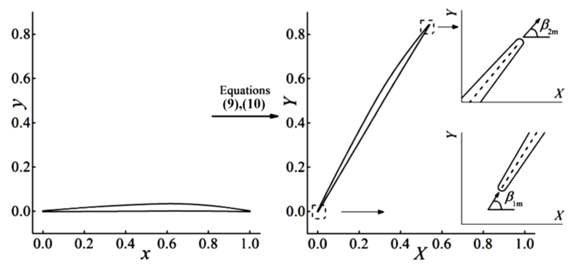
Figure 1.
Schematic for compressor blade (a); airfoil parameter definitions (b).

Figure 2.
Transformation from generated airfoil to staggered airfoil.

Figure 3.
(a) Design frame for ; (b) normalized camber angle distribution samples for different airfoils.
Figure 3.
(a) Design frame for ; (b) normalized camber angle distribution samples for different airfoils.

Figure 4.
Effects of localized adjustable coefficients , (a–d) and (e–h) on sub-function , airfoil shape, blade surface angle and blade passage width distribution .
Figure 4.
Effects of localized adjustable coefficients , (a–d) and (e–h) on sub-function , airfoil shape, blade surface angle and blade passage width distribution .

Figure 5.
(a) Design frame for ; (b) normalized thickness distribution samples for different airfoils.
Figure 5.
(a) Design frame for ; (b) normalized thickness distribution samples for different airfoils.

Figure 6.
Effects of localized adjustable coefficients , and .

Figure 7.
Schematic from airfoils to three-dimensional blade. (a) top view of the airfoil stacking and the geometry definition of sweep and bow, (b) meridian view of the airfoil stacking, (c) front view of the three-dimensional blade.
Figure 7.
Schematic from airfoils to three-dimensional blade. (a) top view of the airfoil stacking and the geometry definition of sweep and bow, (b) meridian view of the airfoil stacking, (c) front view of the three-dimensional blade.

Figure 8.
Meridian view of simulation domain and locations for extracting parameters for performance calculation.
Figure 8.
Meridian view of simulation domain and locations for extracting parameters for performance calculation.

Figure 9.
Grid independency study (a); numerical results and experimental data of Rotor 67 (b).

Figure 10.
Simulated Mach number contours of Rotor 67 at peak efficiency (PE) and near stall (NS).

Figure 11.
Meridian view of the designed transonic axial fan system.

Figure 12.
Inlet Mach number of each blade (a), three-dimensional, top views of designed blades (b) and entire view of the axial fan system (c).
Figure 12.
Inlet Mach number of each blade (a), three-dimensional, top views of designed blades (b) and entire view of the axial fan system (c).

Figure 13.
Rotor 1, important blade geometry design parameter radial distribution (a–c), first segment turning angle and important locations (d), normalized camber angle and thickness distribution (, ) of blade element (e–g).
Figure 13.
Rotor 1, important blade geometry design parameter radial distribution (a–c), first segment turning angle and important locations (d), normalized camber angle and thickness distribution (, ) of blade element (e–g).

Figure 14.
Rotor 1, surface Mach number distribution at relative blade height R = 0.1 (a), 0.3 (b), 0.5 (c), 0.7 (d) and 0.9 (e).
Figure 14.
Rotor 1, surface Mach number distribution at relative blade height R = 0.1 (a), 0.3 (b), 0.5 (c), 0.7 (d) and 0.9 (e).

Figure 15.
Rotor 1, (a) profile of total pressure ratio , (b) diffusion factor DF and (c) adiabatic efficiency .
Figure 15.
Rotor 1, (a) profile of total pressure ratio , (b) diffusion factor DF and (c) adiabatic efficiency .

Figure 16.
Stator 2, important blade geometry design parameter radial distribution (a–c) and normalized camber angle and thickness distribution (, ) of blade element (d–f).
Figure 16.
Stator 2, important blade geometry design parameter radial distribution (a–c) and normalized camber angle and thickness distribution (, ) of blade element (d–f).

Figure 17.
Stator 2, surface Mach number distribution at relative blade height R = 0.1, 0.3, 0.5, 0.7 and 0.9.
Figure 17.
Stator 2, surface Mach number distribution at relative blade height R = 0.1, 0.3, 0.5, 0.7 and 0.9.

Figure 18.
Stator 2, (a) radial distribution of diffusion factor DF, and (b) total pressure recovery coefficient .
Figure 18.
Stator 2, (a) radial distribution of diffusion factor DF, and (b) total pressure recovery coefficient .

Figure 19.
The simulated flow field of the design transonic axial fan component at R = 0.16 (equivalent to the mid location for main-flow path), R = 0.5 and R = 0.9.
Figure 19.
The simulated flow field of the design transonic axial fan component at R = 0.16 (equivalent to the mid location for main-flow path), R = 0.5 and R = 0.9.

Figure 20.
The main-flow aerodynamic characteristic of the design transonic axial fan at relative rotating speed N = 1.0, 0.925 and 0.85, (a) adiabatic efficiency curves; (b) total pressure ratio curves.
Figure 20.
The main-flow aerodynamic characteristic of the design transonic axial fan at relative rotating speed N = 1.0, 0.925 and 0.85, (a) adiabatic efficiency curves; (b) total pressure ratio curves.

Figure 21.
The bypass aerodynamic characteristic of the design transonic axial fan at relative rotating speed N = 1.0, 0.925 and 0.85, (a) adiabatic efficiency curves; (b) total pressure ratio curves.
Figure 21.
The bypass aerodynamic characteristic of the design transonic axial fan at relative rotating speed N = 1.0, 0.925 and 0.85, (a) adiabatic efficiency curves; (b) total pressure ratio curves.


Table 1.
The input parameters for .
| Strength Coefficient | Location Coefficient | Adjustable Coefficients | |
|---|---|---|---|
Table 2.
The input parameters for .
| LE&TE Relative Thickness | Maxim. Thickness Location | Adjustable Coefficients | |||
|---|---|---|---|---|---|
Table 3.
Topology parameters of Grids 1 to 4 for Rotor 67.
| Topology Parameter | Grid 1 | Grid 2 | Grid 3 | Grid 4 |
|---|---|---|---|---|
| Stream-wise nodes | 89 | 129 | 169 | 209 |
| Pitch-wise nodes | 69 | 81 | 101 | 113 |
| Pitch-wise nodes across the O-block | 21 | 29 | 37 | 45 |
| Radial nodes | 61 | |||
| Total nodes of mesh | 1356 k | 2008 k | 2917 k | 3828 k |
Table 4.
One-dimensional design parameter of the efficient transonic axial fan.
| Flow Coefficient, | Load Coefficient, | |
|---|---|---|
| Stage 1 | 0.36 | 0.34 |
| Stage 2 | 0.50 | 0.32 |
| Stage 3 | 0.55 | 0.33 |
Publisher’s Note: MDPI stays neutral with regard to jurisdictional claims in published maps and institutional affiliations. |
© 2021 by the author. Licensee MDPI, Basel, Switzerland. This article is an open access article distributed under the terms and conditions of the Creative Commons Attribution (CC BY) license (https://creativecommons.org/licenses/by/4.0/).
Share and Cite
MDPI and ACS Style
Shi, H. A Parametric Blade Design Method for High-Speed Axial Compressor. Aerospace 2021, 8, 271. https://doi.org/10.3390/aerospace8090271
AMA Style
Shi H. A Parametric Blade Design Method for High-Speed Axial Compressor. Aerospace. 2021; 8(9):271. https://doi.org/10.3390/aerospace8090271
Chicago/Turabian StyleShi, Hengtao. 2021. "A Parametric Blade Design Method for High-Speed Axial Compressor" Aerospace 8, no. 9: 271. https://doi.org/10.3390/aerospace8090271
Note that from the first issue of 2016, this journal uses article numbers instead of page numbers. See further details here.