
Modeling Aircraft Departure at a Runway Using a Time-Varying Fluid Queue


1
Department of Aeronautics and Astronautics, The University of Tokyo, Tokyo 113-8656, Japan
2
Air Traffic Management Department, Electronic Navigation Research Institute, Tokyo 182-0012, Japan
3
Faculty of Aerospace Engineering, Delft University of Technology, 2926 HS Delft, The Netherlands
4
Institute of Logistics and Aviation, Technische Universität Dresden, 01069 Dresden, Germany
*
Author to whom correspondence should be addressed.
Aerospace 2022, 9(3), 119; https://doi.org/10.3390/aerospace9030119
Submission received: 17 December 2021
/
Revised: 17 February 2022
/
Accepted: 22 February 2022
/
Published: 25 February 2022
(This article belongs to the Collection Air Transportation—Operations and Management)
Abstract
:Reducing the length of departure queues at runway entry points is one of the most important requirements for reducing aircraft traffic congestion and fuel consumption at airports. This study designs an aircraft departure model at a runway using a time-varying fluid queue. The proposed model enables us to determine the aircraft waiting time in the departure queue and to evaluate effective control approaches for assigning suitable holds at gates rather than runway entry points. As a case study, this study modeled the departure queue at runway 05 of Tokyo International Airport for an entire day of operations. Using actual traffic data of departures at the airport, the model estimates that aircraft spend a total of 2.5 h departure waiting time in a day at runway 05. Considering the stochastic nature of actual departure traffic, the relevance of the proposed model is discussed using validation criteria. The model estimation shows a reasonable, expected order of magnitude compared with the departure queue recorded in the actual traffic data. Furthermore, ecological and economic benefits are quantitatively evaluated assuming a reduction in the departure queue length. Our results show that about one kiloton of fuel oil per year is wasted due to aircraft waiting to depart from a single departure runway.
1. Introduction
According to estimates of future global air traffic growth, passenger and cargo movements are in high demand on a long-term basis [1]. Congestion reduction at major airports improves operational efficiency and safety while also reducing fuel consumption and delay of arriving and departing air traffic. A bottleneck of the entire air traffic is caused by the runway’s limited capacity. Thus, designing efficient runway management is crucial to accommodate the increasing air traffic demand. The characteristics of the air traffic depend on airport-specific aspects such as runway configurations, taxiways, aprons/ramps, gates, and terminal buildings, geometrical and operational constraints at the surface and the surrounding airspace.
A key operation for airports is aircraft departure management, and in particular “departure metering”, which assigns suitable holds for departure aircraft at their gates [2,3]. The goal of departure metering is to reduce the departure queue at runway entry points while maintaining the runway throughput [4]. As far as the authors are aware, there have been few studies characterizing stochastic features in the aircraft departure process. It is known that the operational uncertainties caused by airport operation impact the efficiency of the departure metering [5,6]. The gate-hold time should be assigned in longer time horizons for improving the performance of departure management [7].
To predict aircraft waiting times at a departure queue, several studies propose queuing models to analyze the taxi-out process of the departure air traffic [4,8,9]. In Reference [8], the authors represent a single departure runway queue using a queuing model assuming that the aircraft arrive at the queue according to a time-dependent schedule and that the service rate follows a time-dependent Erlang distribution. In Reference [9], the authors model airport surface operations of departure air traffic from a single ramp to multiple departure runways using a fluid-flow queuing model. The expected queue length is determined using the flow conservation principle. These queuing networks were used to estimate taxi-out times at three case study airports in the United States [4]. The results showed that the taxi-out times of 60% to 70% flights were estimated within an error margin of 5 min. The accuracy of these estimates, however, impacts the performance of departure metering. For example, departing aircraft take off a takeoff-only runway approximately every two minutes at Tokyo International Airport (RJTT). Thus, simply speaking, an order of the estimation error is desired to be less than a minute for minimizing the departure queue at the runway entry point. Furthermore, for dealing with an integrated arrival and departure control, we need a departure queue model, which allows us to input the time-varying number of departure aircraft entering the runway in a unit time. We also expect that the departure queue model enables us to estimate the optimal departure rate at the runway entry points and to control time-varying arrival and departure rates at the runway approximately 30 to 40 min before the corresponding landing and takeoff.
With this background, there is a challenge of proposing a new departure metering approach targeting an integrated arrival and departure management. For improving the predictability, the push-back and taxi time are estimated using a Machine Learning (ML) model. Based on the estimation, the departure queue is estimated at the runway entry points. The spot-out time of departure aircraft is controlled to maintain the ideal departure rate at the runway entry point for minimizing the estimated departure queue. In this paper, we propose a methodology to develop a departure queue model, which allows us to input the actual time-varying departure rate and to estimate the departure queue under the integrated arrival and departure operation. In line with this, our proposed model applies fluid queues [10,11], where the arrival and service processes of the queuing system follow general distributions. The queue allows us to model time-varying arrival rates and the number of servers (i.e., available runway capacity), which are realistic assumptions when considering the management of departing traffic at airports. In our model, the number of servers corresponds to the rate of runway usage. Using our proposed time-varying fluid queue, this study examines the aircraft waiting time in the departure queue. At the same time, we investigate the best control approaches for departure metering when considering the rate at which aircraft enter the runways and the number of departures held at the gates.
Air traffic incoming/outgoing at airports is typically modeled using queuing models. For example, References [12,13,14,15] propose queuing models focused specifically on runway-related delay and capacity constraints to estimate aircraft arrival delay. Bäuerle et al. [12] calculate the expected waiting time for aircraft arriving at a single runway using an queuing model. In comparison to and models, simple bounds for the expected waiting time are determined. However, in their case study, the authors did not use operational data or compare their results against actual data. Rue and Rosenshine [14] model the arrival of aircraft at Pittsburgh International Airport using and queues. Using semi-Markov decision processes, the authors determine the maximum number of aircraft allowed to land at the airport during peak hours. Bolender and Slater [15] estimate the expected aircraft arrival delay using queues, which yielded reasonable results when compared with numerical simulation data. Furthermore, no comparative analysis with actual flight data was conducted. Long et al. [13] modeled the National Airspace System in the USA as a network of aircraft arriving, taxiing, and departing queues, with TRACON sectors modeled as an queue. The study provided a macroscopic view of the impact of ATM technologies and costs.
In Reference [16], the arrival delay at an airport is analyzed using a queuing model, using two years of radar tracks and flight plans from Tokyo International Airport (RJTT). Herein, a shift from traffic flow to arrival time management indicates capacity enhancements. This initial approach was improved [17] by considering extended arrival management. Approaching the airport, the management of the required inter-arrival times between assigned aircraft (minimum separation standards) and airspace capacities are limiting constraints. The analysis identifies bottleneck areas, where the efficient management of inter-arrival times could mitigate operational delays. The evaluation of different tactical control strategies for RJTT arrivals, 100 NM around the airport, was focused on in Reference [18], using the proposed queuing in comparison to a queuing model. Herein, an improved arrival strategy was suggested considering service times and variances of services times in the airspace areas.
However, these models assume a steady state. In this study, we design an aircraft departure traffic model at runway entry points using fluid queue, with time-varying departure rate and available runway capacity. We demonstrate our model for RJTT departure runway 05 in this paper. The theoretical estimation of the aircraft departure waiting time using the proposed queuing model is discussed against actual traffic data recorded at the airport using validation criteria.
This paper is organized as follows. Section 2 introduces the airport operations at RJTT and examines the current departure queue at the runway entry points of runway 05. The analysis considers recorded aircraft track data for 36 days of operations. These data were recorded in 2019 and 2020 before COVID-19 required the introduction of restrictions on air traffic. Section 3 introduces a fluid queue for the aircraft departure traffic at runway 05. Section 4 applies the model for an entire day of departure traffic at runway 05 and estimates the waiting time of the aircraft in the departure queue at runway 05. The model’s validity is discussed by comparing the obtained theoretical results against actual traffic data recorded at the airport. Section 5 estimates ecological and economical indicators for reducing the departure queue, given the obtained estimates of the departure waiting time. Finally, Section 6 outlines our plans for future extension of the study and provides conclusions.
2. Data Analysis of the Departure Traffic
2.1. Airport Operation at Tokyo International Airport (RJTT)
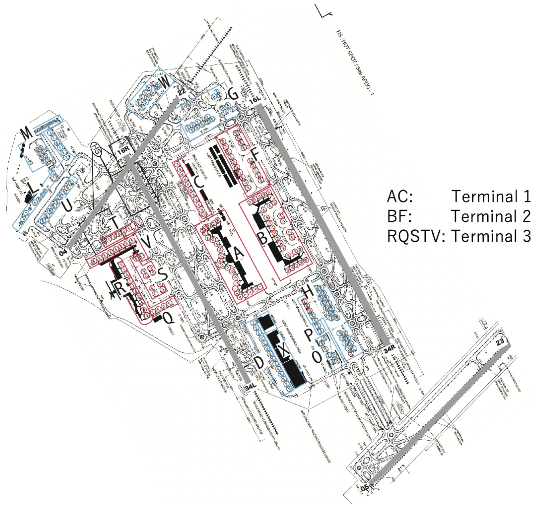
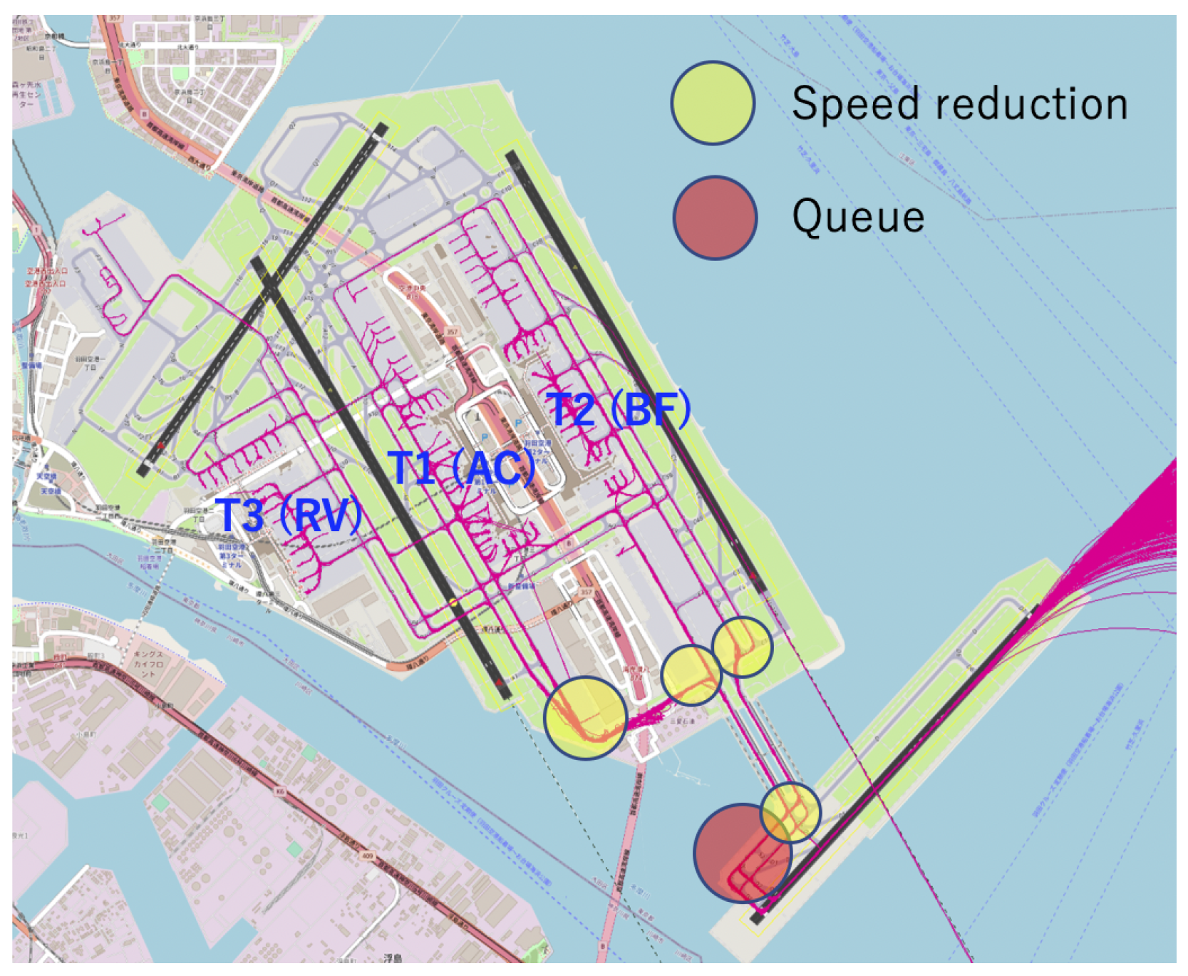
RJTT is Japan’s busiest airport, and the world’s fourth busiest airport by passenger traffic [19]. As shown in Figure 1, the airport has four runways and three terminals.
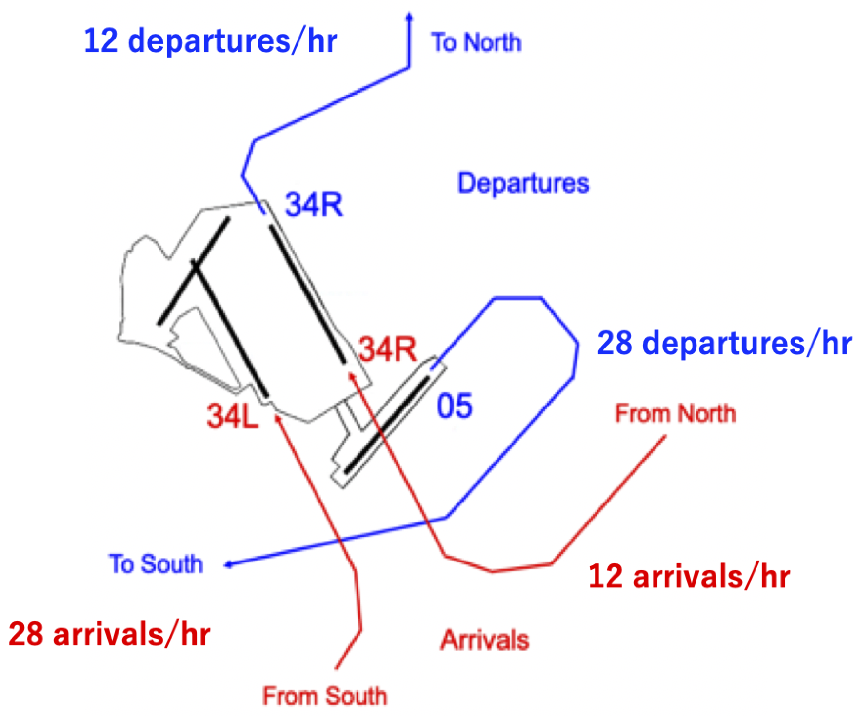
The four runways, a set of parallel north–south runways (34L/16R and 34R/16L) and two southwest–northeast crosswind runways (22/04 and 23/05), are used at RJTT. The use of the runways depends on wind direction. The northerly wind operation accounted for about 70% of the total, taking a larger share than the southerly wind operation. Figure 2 shows the runway usage of departures and arrivals at RJTT in the northerly wind operation. Aircraft arrive at either runway 34L or runway 34R, and departing aircraft takeoff from runway 05 or runway 34R, depending on their origin/destination airports. Runway 05 is used only for departure operation, allowing a maximum of 28 departures in an hour. Runway 34R allows a maximum of 12 departures in an hour. In this study, we focus on the departure traffic at runway 05.
This paper uses 36 days of actual radar data recorded between September 2019 and February 2020. These radar data contain departure and arrival aircraft trajectories, including time, latitude, longitude, and altitude on the surface and at approach and climb phases every second with corresponding aircraft types and call signs. For identifying spot numbers and spot-out time of departure aircraft, we used spot-assignment chart information. All data were provided by the Japan Civil Aviation Bureau (JCAB) of the Japanese Ministry of Land, Infrastructure, Transport, and Tourism for limited use in this study.
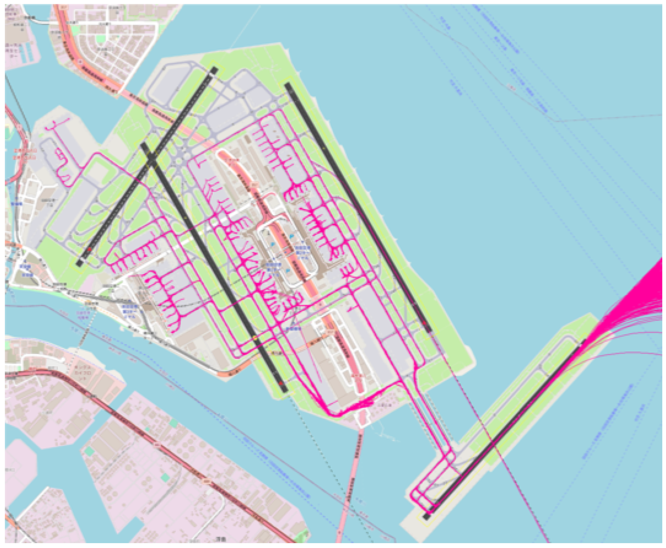
Figure 3 shows aircraft track data on the RJTT surface departing from runway 05 in a day. As shown in Figure 1, three terminals are located and numbered as terminal 3 (T3), T1, and T2 from the east (on the left side of the figure). Domestic flights use T1 and T2, and international flights use T3. 41.2% of aircraft depart from T1, 35.5% in T2, and 11.4% in T3 (R and V gates). Departures from T3 cross runway 34L before reaching the runway, so there is interference with arrivals at runway 34L. As shown in Figure 1, gates/spots are grouped and numbered as A to V; A and C are in T1, B, and F are in T2, and R, Q, S, T, and V are in T3. R and V are mainly used, so we count the aircraft from R and V as T3 departures.
2.2. Departure Traffic Queue at Runway 05
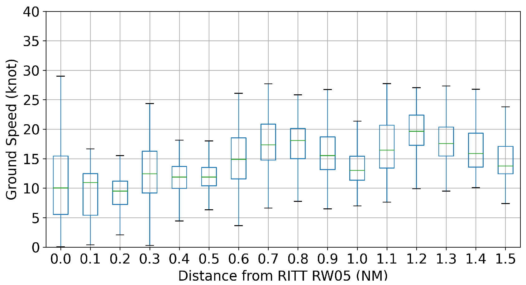
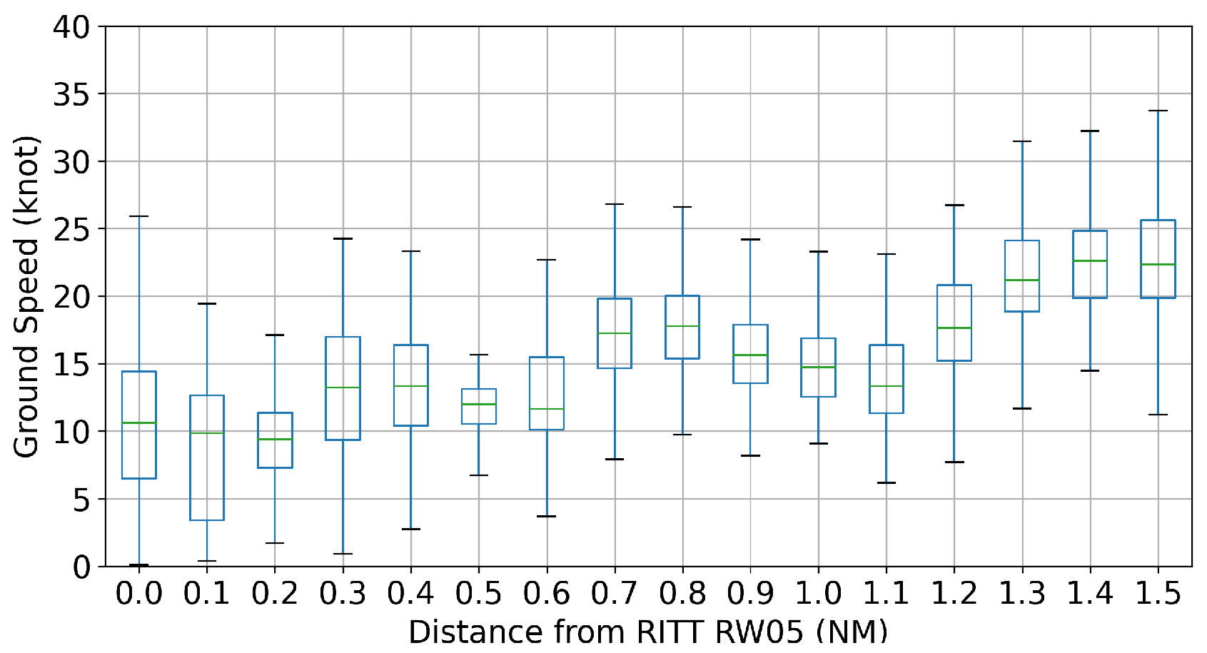
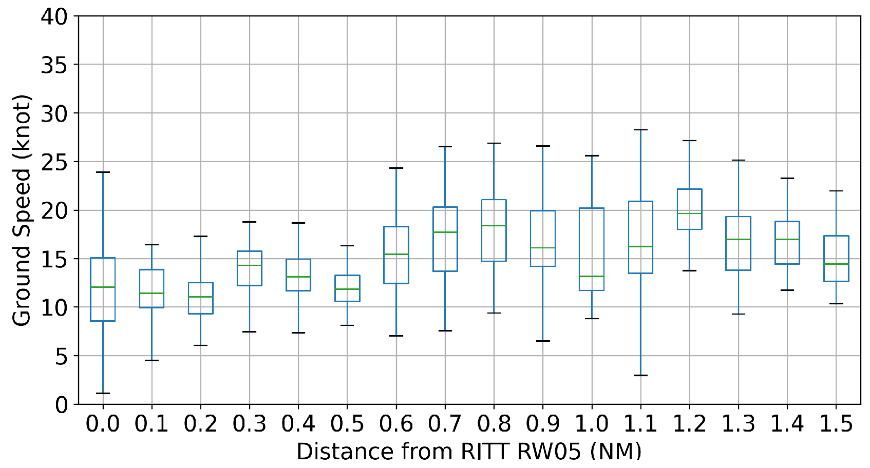
To better understand the departure traffic queue at runway 05, we analyze the stochastic distribution of the ground speed during their surface movement. The ground speed is recorded every 0.1 NM until 2.0 NM distance from the runway entry points of runway 05.
Table 1 summarizes the rate of departure aircraft less than five knots of the ground speed at each location, 0.1 to 0.9 NM distance from the runway entry points every 0.1 NM. “Total” counts all departures at runway 05, and “T1,” “T2,” and “T3” count departures from each terminal. Even though the T3 departure queue is smaller than that of T1 and T2, approximately over 10% of total departures are in the departure queue within 0.3 NM length, and more than 25% are in the departure queue at 0.1 NM. Domestic flights, T1 and T2 departures are highly involved in the departure queue.
Figure 4, Figure 5 and Figure 6 show the ground speed distribution in one day corresponding to departures from T1, T2, and T3 within 1.5 NM distance from the runway entry points every 0.1 NM. As shown in these figures, although the ground speed is variable at each distance, it helps us to understand bottlenecks on the airport surface. Firstly, as shown in Table 1, the departure queue is shown within approximately 0.3 NM from the runway entry points in Figure 5 and Figure 6 because the minimum values are less than five knots. Secondly, the median values are reduced at around 0.5 and 1.0 NM for all terminals and 1.5 NM for T1 and T3 departures. These distance points correspond to the corners on the taxiways, thus the speed is reduced on the surface movements.
Figure 7 visualizes bottlenecks of surface movements in the departure traffic at runway 05 within 1.5 NM distance from the runway entry points based on the analytical results above.
3. Model Description and Formulation
3.1. Modeling Departure Queue at a Single Runway
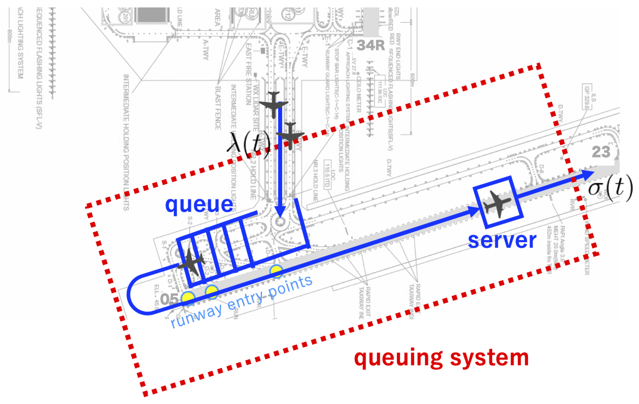
We describe the aircraft departure queue at a single runway, the runway 05 at RJTT in this study, using fluid queue model as follows. We consider the queuing system covering the runway and taxiway within 0.5 NM distance from the runway entry points, as illustrated in Figure 8.
Time-varying arrival rate is counted when the departure aircraft enters the queuing system at 0.5 NM away from the runway 05 entry points; thus, the inter-arrival time is defined as the time between two consecutive departure aircraft entering the system. Service time is given as the sum of Runway Occupancy Time (ROT) and spacing time with the proceeding departure aircraft on the runway entry points. The number of servers , which is given as a time-varying parameter, is defined as the number of departure aircraft allowed to occupy the runway. In this paper, is given because runway 05 is dedicated to only the departures.
3.2. Time-Varying Fluid Queue
In this section, we formulate the aircraft departure queue where based on Whitt et al. [10,11]. Key performance descriptors of the are introduced with two time-varying functions; is the quantity of flow in service at time t, and is the quantity of flow waiting in the queue at t.
Firstly, we determine . The quantity of flow in service at time t, which has been in service for time , is given with the density of flow in service at time t, which has been in service for time , as follows.
Here, .
Secondly, we determine . The quantity of flow waiting in the queue at t, which has been in the queue for time , is given with the density of flow waiting in the queue at time t, which has been waiting in the queue for time , as follows.
Here, .
Using Equations (1) and (2), the initial conditions and are specified with densities and . Then, the total quantity of the flow in the system at t, , is given as follows.
In the model, the total input of the departure traffic into the queuing system over the time interval is , which is given using arrival rate at time u as follows when .
Using Cumulative distribution function (cdf) of service time and the probability density function (pdf) of service time , and are defined as follows.
In this paper, our model consists of the four-tuple of functions; , G, , . All notation of the model is given in Table 2.
3.3. Conditions of Flow in System
This section describes two conditions of the flow in the system, the so-called “under-load (UL)” condition when , and “over-load (OL)” condition when .
3.3.1. UL Condition
In the UL condition, we want two outputs; (i) and (ii) . is defined as “UL terminate time.” It is the time when UL alternates to OL condition.
Firstly, is given as follows using Equations (1), (4) and (5) if the initial quantity in the service is empty, .
Secondly, we assume that the UL condition starts at time when (1) or (2) , and . The UL condition terminates at time , then alternates to the OL condition. The is defined as follows.
Here, the quantity of flow that completes service and leaves the queuing system at time u, in Equation (8) is defined as follows when .
In Equation (9), is given as follows when if , which means that the input flow in service at is 0.
3.3.2. OL Condition
In the OL condition, we require three outputs; (i) , and (ii) , which is defined as “OL terminate time” when the OL condition alternates to UL condition, and (iii) , which is defined as “potential waiting time” of the fluid queue.
Firstly, is given as follows during the OL condition if the initial quantity in the waiting room is empty, .
Secondly we assume that OL condition starts at time when (1) or (2) , and . The OL condition terminates at time , then alternates to UL condition. is given as follows.
In Equation (13), when . is given as follows.
Thirdly, is defined as follows when .
In Equation (15), is the quantity of the flow entering service during the time interval and is given as follows when .
3.4. Aircraft Departure Waiting Time
In this study, we define aircraft departure waiting time in Equation (15).
As another index to approximate the total waiting time of departure aircraft during the estimation time, including m times OL periods, we define as follows.
In Equation (17), is the mean of during the i th OL period. is the number of departure aircraft entering the system during the i th OL period.
4. Estimating Departure Queues
4.1. Stochastic Features in the Queuing Model
4.1.1. Arrival Rate
We applied the proposed departure queue model for a day operation at runway 05 for estimating the departure queue. As a case study, stochastic features under the nominal operation on 15 November 2019 were selected and implemented into the model. We selected the case study day because a nominal and north-wind operation was conducted all over the day.
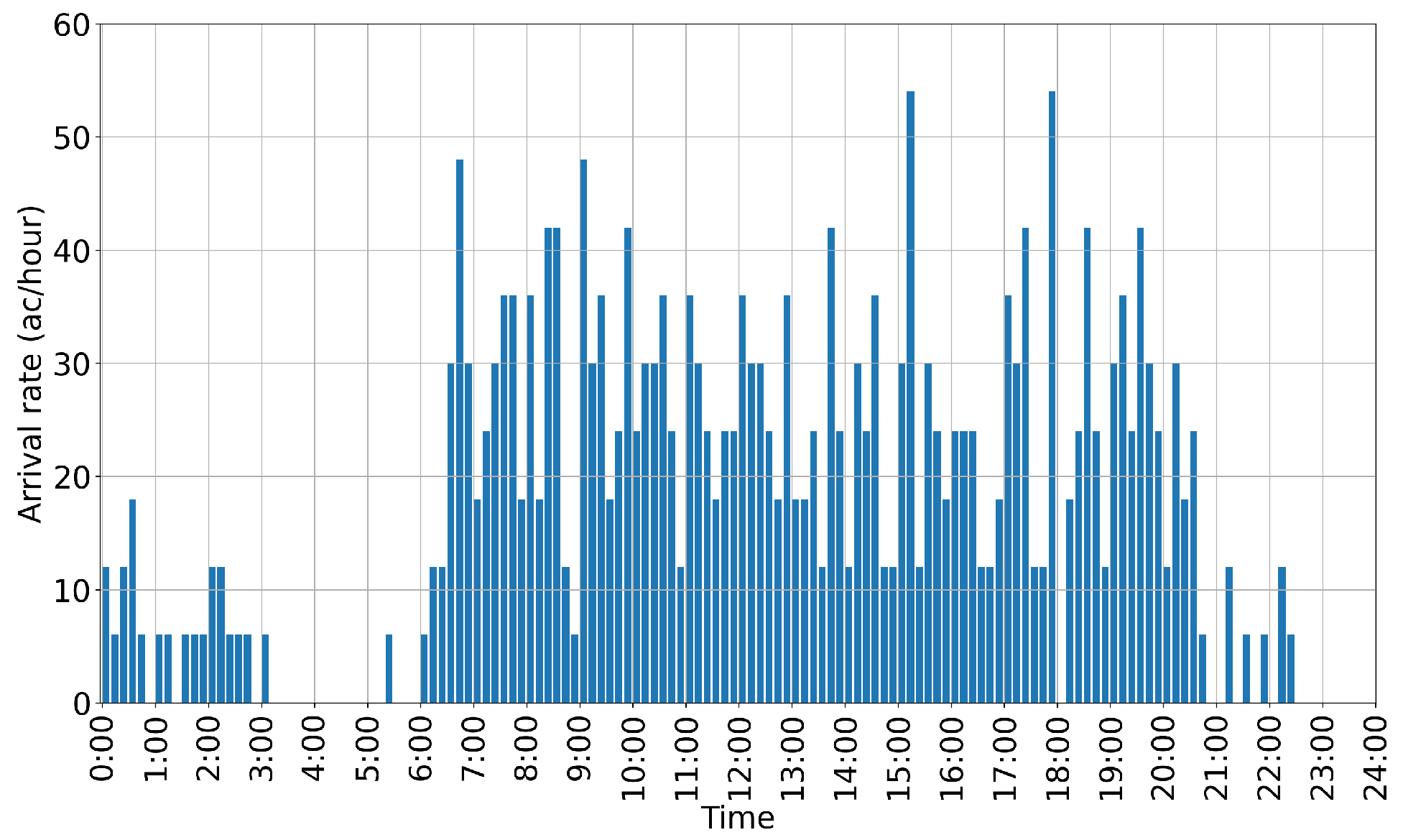
Figure 9 shows aircraft arrival rate in an hour at the queuing system, which means that the number of departure aircraft counted at 0.5 NM away from the runway entry points in an hour. The arrival rate is given as an average in 10 min intervals in this study. The given in an hour is where min and . Here, is a counted number of departure aircraft at 0.5 NM away from the runway entry points between time and . As shown in Figure 9, is time-varying in 10 min intervals all over the day, although the maximum runway throughput is fixed as 28 departures in an hour.
4.1.2. Service Time
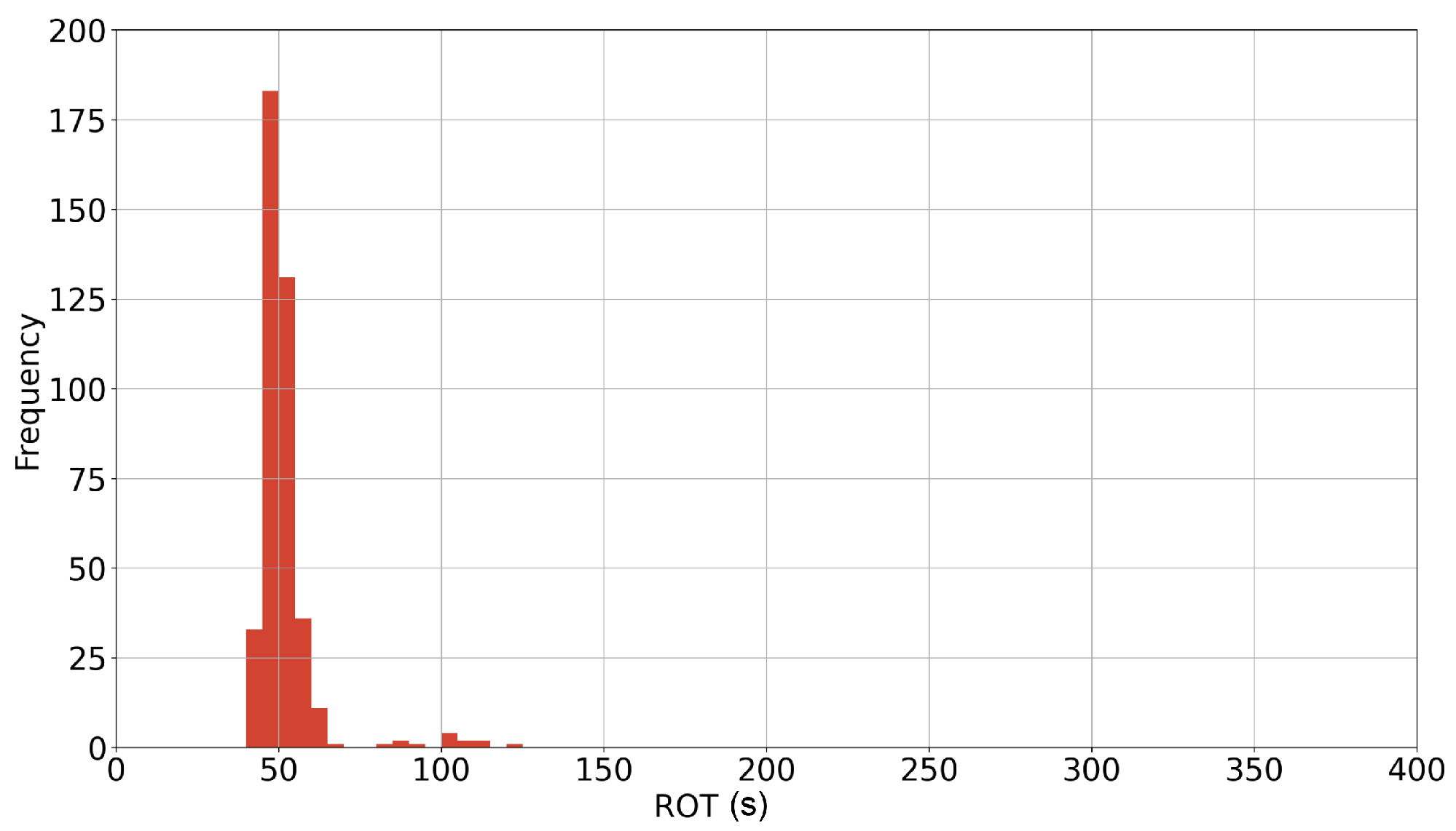
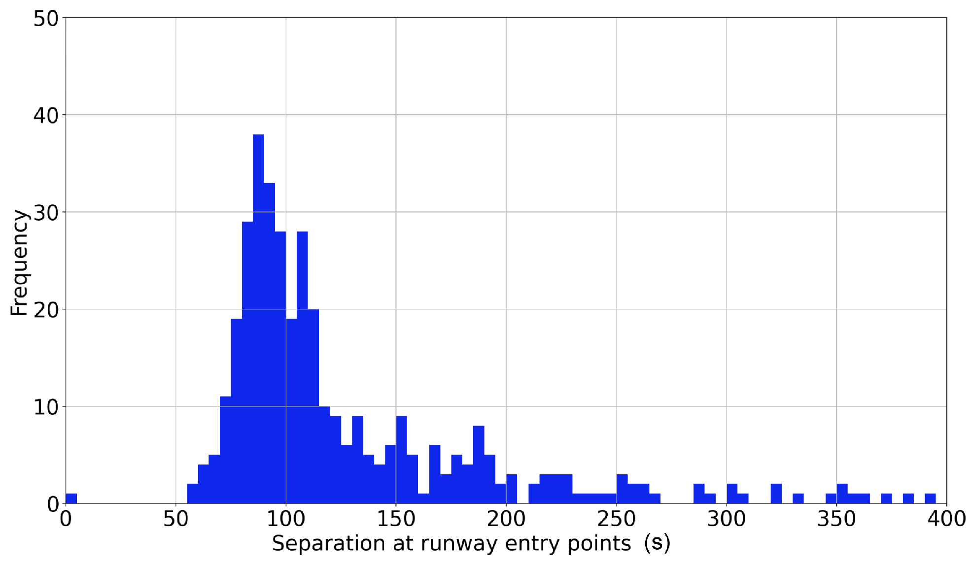
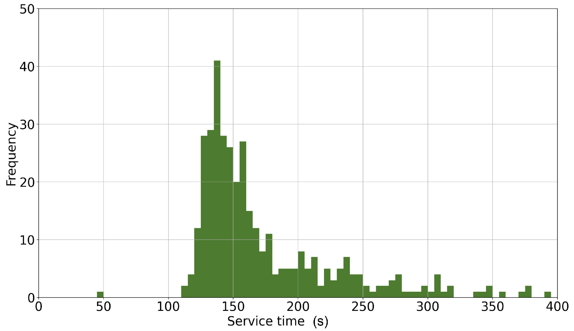
The service time is the time that the runway is unavailable to other departures in our model. Ideally, it is decided by the minimum separation rules (e.g., the sum of the time in which a leading aircraft is clear of the runway and the time of the wake vortex separation), but it is not in the case of the actual operation at RJTT. According to the runway capability (the maximum 28 departures in an hour at RW05) and interference with the other aircraft traffic, on average, approximately 130 s are given to the departure separation, which is the sum of ROT and time separation at the runway entry point. Thus, in our model in Section 3.1, the service time is defined as the sum of ROT and separation time at the runway entry points using the aircraft track data, which recorded actual departure time separation.
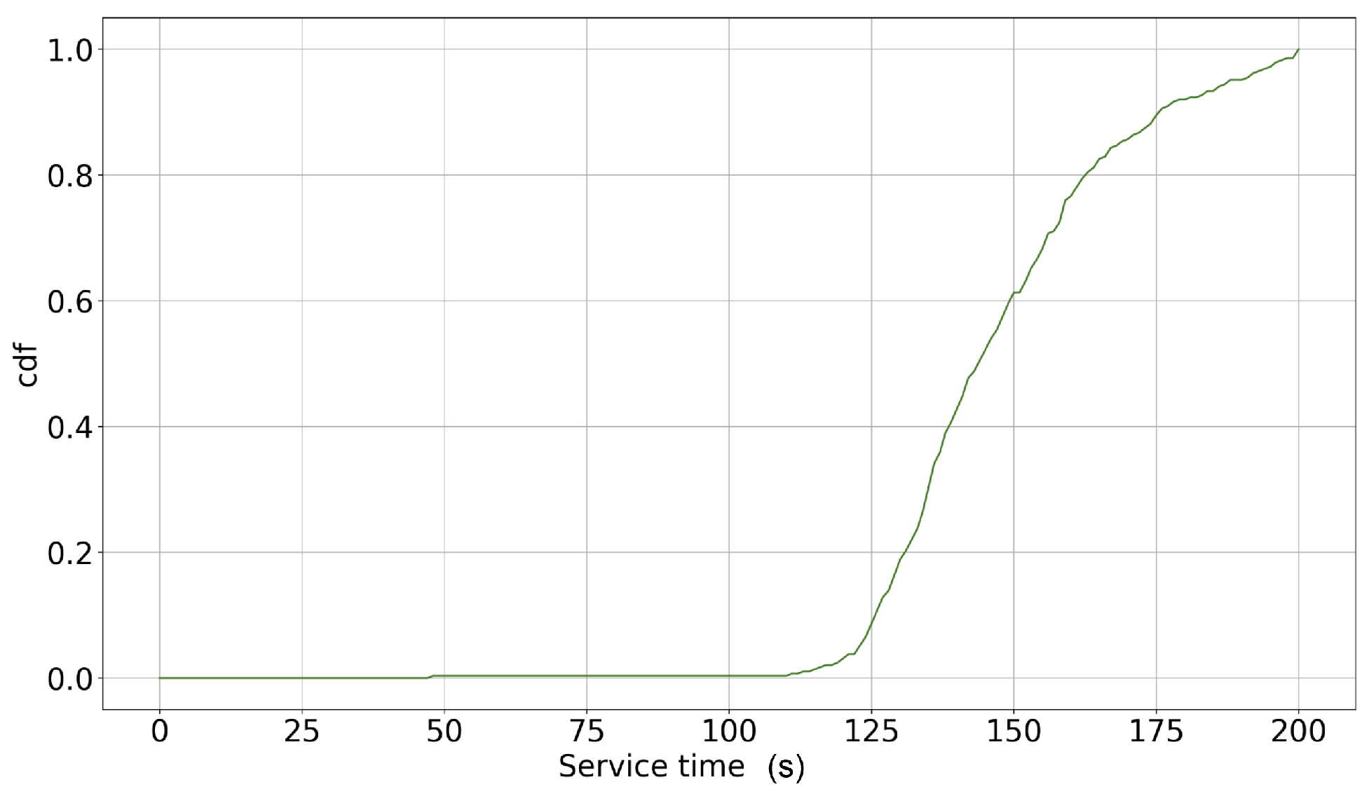
A histogram of the ROT and separation time is shown in Figure 10 and Figure 11. The tail of the histogram is extended in Figure 11 because the departure separation grows wider when the departure rate at the runway is small during low demands. Figure 12 shows a histogram of service time. Furthermore, some aircraft stay within the 0.5 NM distance areas for reasons other than waiting for subsequent departures, such as aircraft maintenance. For avoiding the impact of extremely long departure separation time, our model considers the service time of fewer than 200 s in this study. Figure 13 shows CDF of service time, . We use the stochastic distribution for estimating states and waiting time of the departure queues in the following section.
4.2. Time-Varying States in the Departure Queue
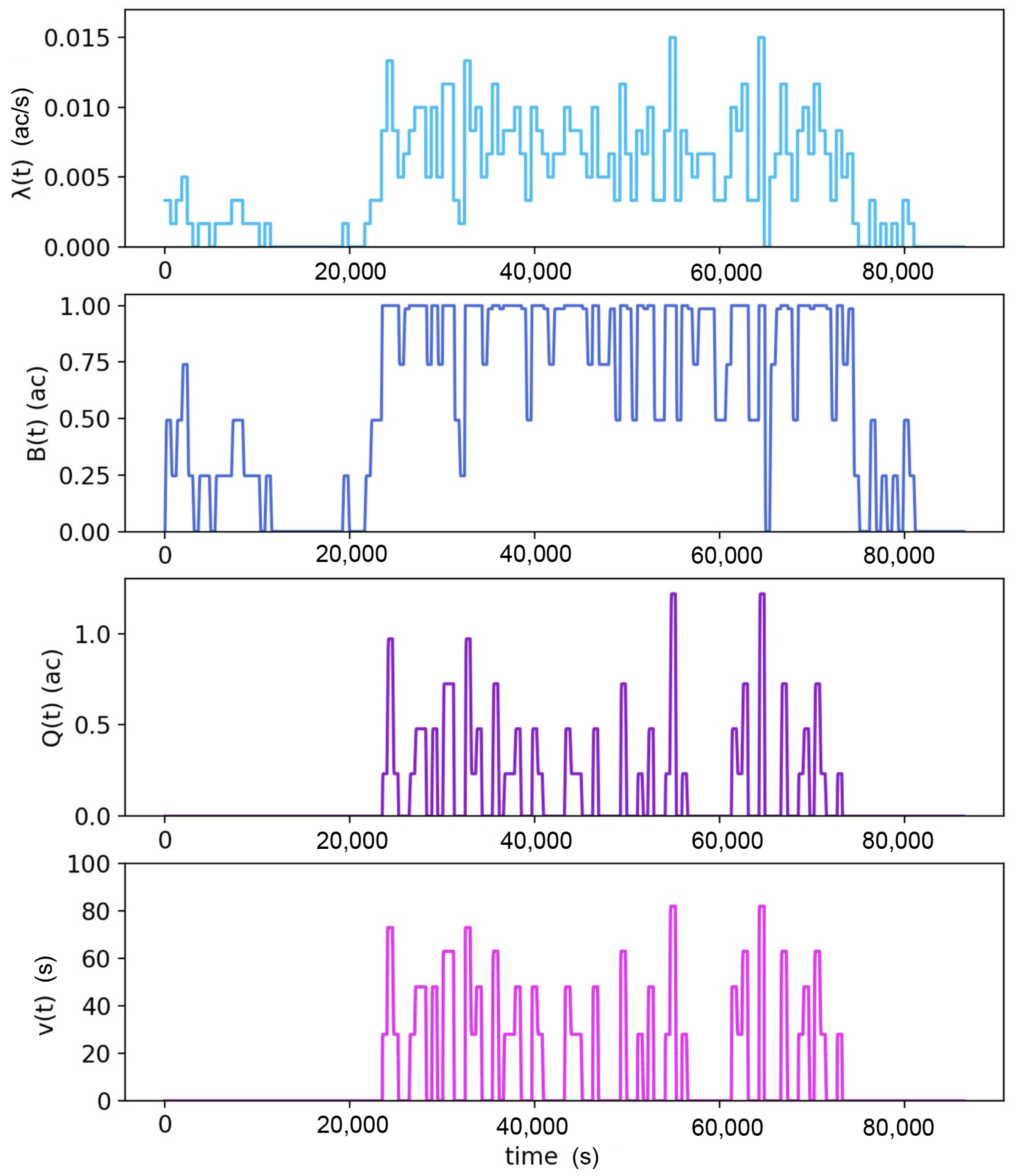
Using the stochastic features in Section 4.1, this section estimates time-varying states; and . Simultaneously, we obtain the ith OL starting time , terminate time , and time intervals .
Figure 14 shows the results that estimate time-varying states of the departure queue in a day. A total of 21 OL periods are counted. During the OL periods , as shown in Figure 14. Since is given as the average arrival rate in 10 min time interval, the value of and are also given as the average every 10 min. The maximum is 1.22, indicating that 1.22 departures have been waiting in the departure queue on an average for 10 min.
Figure 14 also indicates that the variance in the time-varying arrival rate is the cause of the OL conditions. It gives us insights that controlling the arrival rate among the 10-minute windows can dramatically reduce the OL periods and aircraft departure waiting time.
According to the model definition, it is difficult to extract the time-varying states , , and from the actual data and to compare them with the results of the model estimation in Figure 14. Despite comparing the time-varying states in the context of model validation, this paper introduces a validation criterion in Section 4.4, which evaluates the relevance of the model estimation using actual operational data.
4.3. Departure Waiting Time in the Queue
Table 3 summarizes the value of the ith OL time intervals , the aircraft departure waiting time and total aircraft departure waiting time in the intervals. The maximum OL time interval is estimated to be 1950 s in the 7th OL interval between 10:00 and 1:00 a.m. (because corresponds to 10:42:39 a.m.). The maximum departure waiting time in 10 min average is 82 s in the 14th and 17th OL interval, which occurred between 15:00 and 19:00 ( and ). Thus, the proposed model enables us to estimate the aircraft departure waiting time in the queue and the OL start and end times.
4.4. Model Validation
The reasoning behind the model validation is complicated for the following reasons. Firstly, it is difficult to extract waiting time in the departure queue defined in the queuing model from actual traffic data. It is because our queuing model estimates the waiting time within 0.5 NM range from the runway entry point except for departure separation time. In the departure traffic data within 0.5 NM range from the runway entry point, the time records consist of a sum of taxi-time, separation time, and the waiting time, including each variation. Secondly, it is difficult to realize these stochastic data in a numerical simulation environment because the main cause of the data variation is based on the human operation, i.e., air traffic controllers and pilot’s control. Thus, we introduce validation criteria, which evaluate the relevance of the model using actual operational data in this section.
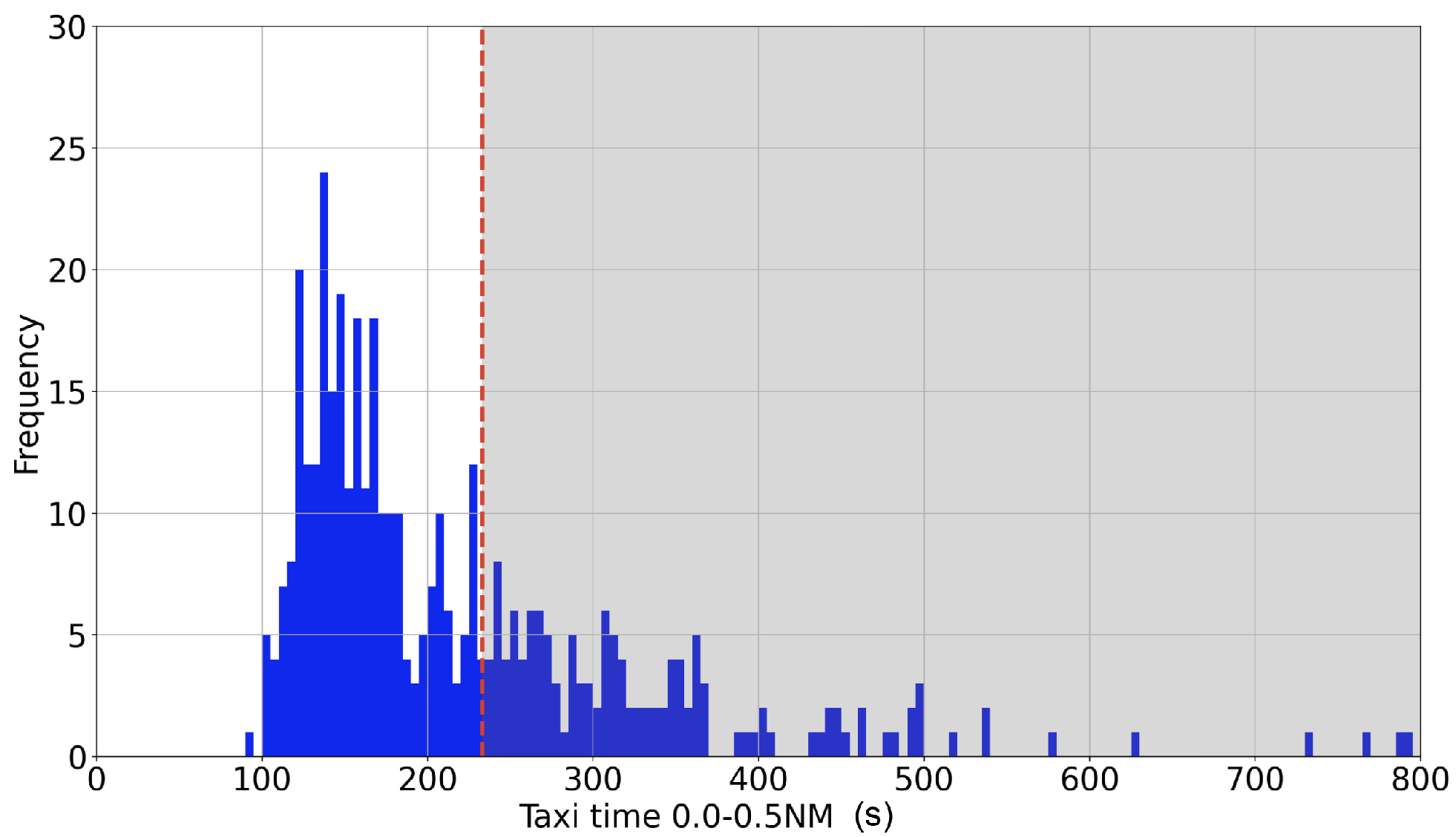
For validating the departure queue model, we compare the taxi time of the departure aircraft in the actual data with the estimated results as follows. Figure 15 shows a data histogram of the taxi time within 0.5 NM from the runway 05 entry point. As a benchmark to approximate the taxi time of the departure aircraft using the estimated departure waiting time, is defined in the criteria as follows.
is given as an index that measures time intervals when the departures are within 0.5 NM area from the runway entry point. Here, is the separation time between the proceeding aircraft at the runway threshold at t as shown in Figure 11. is the minimum taxi time of departures with service time s, which corresponds to the available taxi time of departures in low traffic demands, as defined in Section 4.1.2. In the calculation, we assume , which corresponds to the average waiting time estimated in each ith OL period.
Using departure traffic data in the day, s is given. Assuming the departures of which taxi time is larger than (see the grayscale in Figure 15), 23% of departures were in the queue before takeoff. As shown in Section 2.2, 26% of total departures were estimated in the queue at 0.1 NM (see Table 1). Compared with the data analysis in Section 2.2, the scale of estimation is relevant. When the departure aircraft are in the queue when s and satisfies s, an estimated sum of corresponding to departures in the queue is 23,646 s. In the actual data corresponding to the same departures, a sum of taxi time within 0.5 NM area from the runway entry point is 22,606 s. This comparison explains that the model estimation grasps the features of the actual departure queue because the scale of the error is within 5 %.
5. Estimating Ecological and Economical Impacts Due to Departure Queue
One of the important questions asked by airlines and airport operators is the available amount of fuel reduction according to minimizing the departure queue at the runway entry point. Thus, we discuss the impacts of fuel consumption due to the departure queue at the single runway of RJTT in this paper.
The process of estimating the ecological and economic impacts is carried out in three steps. (1) We determine average fuel flow at the airport using the rate of aircraft types at the airport and the idling fuel flow of the corresponding aircraft types. (2) We obtain the total fuel consumption due to the departure queue in a day by multiplying and . (3) Economic impacts in a day are estimated by multiplying the oil price with the total fuel consumption given in the previous step.
According to the representative engines corresponding to aircraft types arriving/departing at/from RJTT, fuel flow in seconds is given in Table 4 using the ICAO engine emissions databank [21]. We estimated the average fuel flow on the surface operation at RJTT (kg/s) using the rate of the kth aircraft type at RJTT (here ), (0.01%), and the fuel flow of the kth aircraft type when the engine is idle, (kg/s), in Table 4.
The average fuel flow on the surface operation, in Equation (19), is estimated as 0.32 kg/s per flight at RJTT. Compared with other airports, the values estimated using the ICAO databank [21] and Equation (19) were found to be 0.20 kg/s for Newark Liberty International airport and Dallas Fort Worth International airport, and 0.17 kg/s at Charlotte Douglas International airport as shown in [4]. Due to the lower fraction of regional jets, the value of fuel flow at RJTT is higher than the comparison airports.
Applying the departure queue model, a total of seven days of is given by Equation (17), which is the total aircraft departure delay time in the queue, are estimated. Table 5 summarizes the and a corresponding value of the fuel consumption for every seven case study days given by .
The daily average of the total fuel consumption in the seven days is 2.7 tons based on the values in Table 5. With linear interpolation, 985 tons of fuel is wasted annually per one departure runway. It is translated into almost USD 1.7 million (JPY 1.85 billion) applying the current price of fuel oil (JPY 150 per litter).
6. Conclusions
This study proposed an aircraft departure model at a runway using a time-varying fluid queue. The proposed model enables us to design departure traffic flow with two time-varying control inputs, the arrival rate and the number of servers at/in the departure queuing system and to evaluate the effectiveness of the departure traffic control by quantitatively assessing the waiting time in the queue. As a case study, the fluid queue model with a time-constant server was successfully implemented into the aircraft departure queue at runway 05 of Tokyo International Airport. The results showed that an average of 2.5 h waiting time was estimated in a day operation. The relevance of the departure queue model was discussed by comparing it with the stochastic features of the actual operational data using validation criteria. Ecological and economic benefits of reducing the departure queue were discussed based on the quantitative estimation. These quantitative estimations clarified the target to achieve by implementing our design departure metering system.
This paper developed a methodology to model departure queues and pointed out challenges. In future studies, the authors plan to develop the departure queue model and validation method and examine the best departure metering approach, which is applicable in the actual airport operations and system design. More specifically, the best departure metering logic will be proposed by controlling two time-varying parameters; (1) arrival rate at the queuing system and (2) service rate at the runway. For reducing uncertainties in the taxi and push-pack estimation, ML approaches will be integrated into the departure metering logic. The proposed model will be used for both departure and arrival aircraft on a runway. It enables us to discuss the future integrated control of arrival and departure queues. On the safety aspect of view, simulation experiments will be conducted to evaluate the impacts of the proposing approach. We will take into account the comments of air traffic controllers and airlines on the application.
Author Contributions
Conceptualization, E.I. and M.S.; methodology, E.I. and M.S.; validation, E.I.; formal analysis, E.I.; investigation, E.I.; resources, E.I.; data E.I.; writing—original draft preparation, E.I., M.M. and M.S.; writing—review and editing, E.I., M.M. and M.S.; project administration, E.I.; funding acquisition, E.I. All authors have read and agreed to the published version of the manuscript.
Funding
This research was supported by ENRI project “Studies on the AMAN/DMAN/SMAN integration”. It was also supported by JSPS KAKENHI Grant Number 20H04237.
Acknowledgments
This research was conducted under CARATS initiatives supported by the Civil Aviation Bureau (JCAB) of the Japanese Ministry of Land, Infrastructure, Transport, and Tourism. The authors are grateful to JCAB for providing air traffic data.
Conflicts of Interest
The authors declare no conflict of interest. The funders had no role in the design of the study; in the collection, analyses, or interpretation of data; in the writing of the manuscript, or in the decision to publish the results.
References
- IATA. COVID-19 Outlook for Air Travel in the Next 5 Years; IATA: Montreal, QC, Canada, 2020. [Google Scholar]
- FAA Surface CDM Team. US Airport Surface Collaborative Decision Making (CDM) Concept of Operations (ConOps) in the Near-Term: Applications of Surface CDM at United States Airports; FAA Surface CDM Team: Washington, DC, USA, 2012. [Google Scholar]
- EUROCONTROL Airport CDM Team. Airport CDM Implementation-The Manual; EUROCONTROL Airport CDM Team: Brussels, Belgium, 2018. [Google Scholar]
- Badrinath, S.; Balakrishnan, H.; Joback, E.; Reynolds, T. Impact of Off-Block Time Uncertainty on the Control of Airport Surface Operations. Transp. Sci. 2020, 54, 855–1152. [Google Scholar] [CrossRef]
- Ball, M.; Vossen, T.; Hoffman, R. Analysis of demand uncertainty effects in ground delay programs. In Proceedings of the 4th USA/Europe Air Traffic Management R & D Seminar, Santa Fe, NM, USA, 4–7 December 2001. [Google Scholar]
- McFarlanee, P.; Balakrishnan, H. Optimal control of airport pushbacks in the presence of uncertainties. In Proceedings of the American Control Conference, Boston, MA, USA, 6–8 July 2016. [Google Scholar]
- Liu, Y.; Hansen, M.; Gupta, G.; Malik, W.; Jung, Y. Predictability impacts of airport surface automation. Transp. Res. Part C Emerg. Technol. 2014, 44, 128–145. [Google Scholar] [CrossRef]
- Simaiakis, I.; Balakrishnan, H. A queuing model of the airport departure process. Transp. Sci. 2015, 50, 94–109. [Google Scholar] [CrossRef]
- Badrinath, S.; Li, M.; Balakrishnan, H. Integrated surface—Airspace model of airport departures. J. Guid. Control. Dyn. 2018, 42, 1049–1063. [Google Scholar] [CrossRef]
- Liu, Y.; Whitt, W. The Gt/GI/st+GI many-server fluid queue. Queuing Syst. 2012, 71, 405–444. [Google Scholar] [CrossRef] [Green Version]
- Whitt, W. Time-Varying Queues. Oueueing Model. Serv. Manag. 2018, 1, 79–164. [Google Scholar]
- Bäuerle, N.; Engelhardt-Funke, O.; Kolonko, M. On the waiting time of arriving aircrafts and the capacity of airports with one or two runways. Eur. J. Oper. Res. 2007, 177, 1180–1196. [Google Scholar] [CrossRef] [Green Version]
- Long, D.; Johnson, J.; Gaier, E.M.; Kostiuk, P.F. Modeling Air Traffic Management Technologies with a Queuing Network Model of the National Airspace System; NASA Langley Technical Report Server: Washington, DC, USA, 1999. [Google Scholar]
- Rue, R.C.; Rosenshine, M. The application of semi-Markov decision processes to queuing of aircraft for landing at an airport. Transp. Sci. 1985, 19, 154–172. [Google Scholar] [CrossRef]
- Bolender, M.; Slater, G. Evaluation of scheduling methods for multiple runways. J. Aircr. 2000, 37, 410–416. [Google Scholar] [CrossRef] [Green Version]
- Itoh, E.; Mitici, M. Queue-based Modeling of the Aircraft Arrival Process at a Single Airport. Aerospace 2019, 6, 103. [Google Scholar] [CrossRef] [Green Version]
- Itoh, E.; Mitici, M. Analyzing Tactical Control Strategies for Aircraft Arrivals at an Airport Using a queuing Model. J. Air Transp. Manag. 2020, 89, 101938. [Google Scholar] [CrossRef]
- Itoh, E.; Mitici, M. Evaluating the Impact of New Aircraft Separation Minima on Available Airspace Capacity and Arrival Time Delay. Aeronaut. J. 2020, 124, 447–471. [Google Scholar] [CrossRef] [Green Version]
- Airports Council International (ACI). Passenger Traffic 2017 FINAL (Annual). In Passenger Summary; Airports Council International: Montreal, QC, Canada, 2019. [Google Scholar]
- Ministry of Land, Infrastructure, Transport and Tourism. AIS Japan—Japan Aeronautical Information Service Center. 2021. Available online: https://aisjapan.mlit.go.jp (accessed on 27 January 2022).
- ICAO. ICAO Engine Emissions Databank. 2018. Available online: https://www.easa.europa.eu/easa-and-you/environment/icao-aircraft-engine-emissions-databank (accessed on 31 July 2021).
Figure 1.
RJTT surface configuration [20].
Figure 1.
RJTT surface configuration [20].

Figure 2.
RJTT northerly wind operation.

Figure 3.
RJTT departures from Runway 05.

Figure 4.
GS distribution of departures from T1.

Figure 5.
GS distribution of departures from T2.

Figure 6.
GS distribution of departures from T3 (R and V).

Figure 7.
Bottlenecks of RJTT departures within 1.0 NM from Runway 05 entry points.

Figure 8.
Modeling the RJTT Runway 05 departure queue.

Figure 9.
Arrival rate at the queuing system.

Figure 10.
Runway occupancy time (ROT).

Figure 11.
Separation time at runway entry points.

Figure 12.
Service time.

Figure 13.
Service time cdf, .

Figure 14.
Time-varying states in the departure queue, , , , and in the ith OL period in one day.

Figure 15.
Determining departures waiting in the queue based on taxi time within 0.5 NM from the runway 05 entry points.
Figure 15.
Determining departures waiting in the queue based on taxi time within 0.5 NM from the runway 05 entry points.


Table 1.
Rate of departure counts corresponding to the aircrafts with less than 5 knot ground speed recorded every 0.1 NM until 0.9 NM distance from the runway entry points of runway 05.
Table 1.
Rate of departure counts corresponding to the aircrafts with less than 5 knot ground speed recorded every 0.1 NM until 0.9 NM distance from the runway entry points of runway 05.
| Distance (NM) | 0.1 | 0.2 | 0.3 | 0.4 | 0.5 | 0.6 | 0.7 | 0.8 | 0.9 |
|---|---|---|---|---|---|---|---|---|---|
| Total (%) | 26 | 10 | 9.9 | 5.0 | 2.6 | 1.4 | 0.75 | 0.35 | 0.15 |
| T1 (%) | 27 | 11 | 10 | 5.4 | 2.8 | 1.4 | 0.71 | 0.30 | 0.24 |
| T2 (%) | 29 | 11 | 10 | 5.6 | 3.0 | 1.5 | 0.83 | 0.35 | 0.043 |
| T3 (%) | 16 | 6.6 | 10 | 2.4 | 1.2 | 0.95 | 0.68 | 0.47 | 0.14 |
Table 2.
Notation of the model.
| Parameter | Description |
|---|---|
| B | Quantity of flow in service |
| b | Density of flow in service |
| Q | Quantity of flow waiting in the queue |
| q | Density of flow waiting in the queue |
| X | Total quantity of the flow in the system |
| Total of arrival flow (departure traffic flow) into the system | |
| Arrival rate at the system | |
| G | Cumulative distribution function of service time |
| g | Probability density function of service time |
| Parameter defined in Equation (5) | |
| Parameter defined in Equation (6) | |
| Over Load (OL) terminate time | |
| OL start time | |
| Under Load (UL) terminate time | |
| UL start time | |
| Quantity of flow which completes service | |
| v | Waiting time |
| E | Quantity of flow entering service |
Table 3.
OL time intervals and departure waiting times in one day.
| i | (s) | (s) | (s) | (Aircraft) | (s) |
|---|---|---|---|---|---|
| 1 | 25,270 | 1768 | 73 | 17 | 734 |
| 2 | 28,296 | 1887 | 48 | 16 | 627 |
| 3 | 29,496 | 643 | 48 | 5 | 213 |
| 4 | 31,288 | 1248 | 63 | 13 | 774 |
| 5 | 34,296 | 1831 | 73 | 18 | 869 |
| 6 | 36,166 | 763 | 63 | 8 | 415 |
| 7 | 38,559 | 1950 | 48 | 14 | 454 |
| 8 | 40,947 | 1270 | 48 | 10 | 351 |
| 9 | 45,147 | 1942 | 48 | 17 | 553 |
| 10 | 46,896 | 643 | 48 | 7 | 298 |
| 11 | 49,966 | 705 | 63 | 6 | 321 |
| 12 | 51,747 | 645 | 28 | 5 | 121 |
| 13 | 52,872 | 667 | 48 | 6 | 252 |
| 14 | 55,305 | 1203 | 82 | 10 | 542 |
| 15 | 56,547 | 645 | 28 | 6 | 145 |
| 16 | 63,088 | 1835 | 63 | 16 | 716 |
| 17 | 64,882 | 638 | 82 | 6 | 418 |
| 18 | 67,366 | 763 | 63 | 5 | 259 |
| 19 | 69,759 | 1257 | 48 | 9 | 322 |
| 20 | 71,547 | 1344 | 63 | 13 | 541 |
| 21 | 73,270 | 568 | 28 | 4 | 103 |
Table 4.
Aircraft types, rate, and fuel consumption per engine [21].
Table 4.
Aircraft types, rate, and fuel consumption per engine [21].
| k | Aircraft Type | Rate (%) | Fuel Flow (kg/s) |
|---|---|---|---|
| 1 | B738 | 34 | 0.097 |
| 2 | B763 | 18 | 0.20 |
| 3 | B772 | 14 | 0.21 |
| 4 | A320 | 10 | 0.10 |
| 5 | B788 | 6 | 0.21 |
| 6 | B773 | 3 | 0.34 |
| 7 | B77W | 3 | 0.30 |
| 8 | B789 | 2 | 0.23 |
| 9 | A321 | 2 | 0.11 |
| 10 | B737 | 2 | 0.12 |
| 11 | A333 | 2 | 0.26 |
| 12 | E170 | 1 | 0.060 |
| 13 | A332 | 0.6 | 0.259 |
| 14 | B744 | 0.5 | 0.228 |
| 15 | B734 | 0.4 | 0.124 |
| 16 | Others | 0.8 | 0.089 |
Table 5.
Total departure delay in each of seven case study days.
| Case Study Day | (h) | Fuel Consumption (ton) |
|---|---|---|
| Day 1 | 2.51 | 2.89 |
| Day 2 | 2.64 | 3.04 |
| Day 3 | 1.77 | 2.04 |
| Day 4 | 2.62 | 3.02 |
| Day 5 | 2.60 | 3.00 |
| Day 6 | 2.12 | 2.44 |
| Day 7 | 2.15 | 2.48 |
Publisher’s Note: MDPI stays neutral with regard to jurisdictional claims in published maps and institutional affiliations. |
© 2022 by the authors. Licensee MDPI, Basel, Switzerland. This article is an open access article distributed under the terms and conditions of the Creative Commons Attribution (CC BY) license (https://creativecommons.org/licenses/by/4.0/).
Share and Cite
MDPI and ACS Style
Itoh, E.; Mitici, M.; Schultz, M. Modeling Aircraft Departure at a Runway Using a Time-Varying Fluid Queue. Aerospace 2022, 9, 119. https://doi.org/10.3390/aerospace9030119
AMA Style
Itoh E, Mitici M, Schultz M. Modeling Aircraft Departure at a Runway Using a Time-Varying Fluid Queue. Aerospace. 2022; 9(3):119. https://doi.org/10.3390/aerospace9030119
Chicago/Turabian StyleItoh, Eri, Mihaela Mitici, and Michael Schultz. 2022. "Modeling Aircraft Departure at a Runway Using a Time-Varying Fluid Queue" Aerospace 9, no. 3: 119. https://doi.org/10.3390/aerospace9030119
Note that from the first issue of 2016, this journal uses article numbers instead of page numbers. See further details here.