
OpenAP.top: Open Flight Trajectory Optimization for Air Transport and Sustainability Research


Faculty of Aerospace Engineering, Delft University of Technology, 2629 HS Delft, The Netherlands
Aerospace 2022, 9(7), 383; https://doi.org/10.3390/aerospace9070383
Submission received: 20 June 2022
/
Revised: 12 July 2022
/
Accepted: 13 July 2022
/
Published: 15 July 2022
(This article belongs to the Collection Air Transportation—Operations and Management)
Abstract
:Trajectory optimization has been an active area of research for air transport studies for several decades. But almost all flight optimizers proposed in the literature remain close-sourced, which presents a major disadvantage for the advancement of scientific research. This optimization depends on aircraft performance models, emission models, and operational constraints. In this paper, I present a fully open trajectory optimizer, OpenAP.top, which offers researchers easy access to the complex but efficient non-linear optimal control approach. Full flights can be generated without specifying flight phases, and specific flight segments can also be independently created. The optimizer adapts to meteorological conditions and includes conventional fuel and cost index objectives. Based on global warming and temperature potentials, its climate objectives form the basis for climate optimal air transport studies. The optimizer’s performance and uncertainties under different factors like varying mass, cost index, and wind conditions are analyzed. Overall, this new optimizer brings a high performance for optimal trajectory generations by providing four-dimensional and wind-enabled full-phase optimal trajectories in a few seconds.
1. Introduction
Air transportation contributes between 3% and 5% of global greenhouse gas emissions. Aviation emissions also create a greater impact due to the altitude of emissions. Research focusing on the operation aspect of air transport often requires the knowledge of climate-optimal trajectories.
Over the past decades, many studies have addressed the optimization of flight trajectories [1]. Traditionally, the objective of flight trajectory optimization in transport studies has been centered around the balance between fuel consumption and flight time, which is modeled by the cost index [2,3]. The cost index describes the weight of fuel and time. A flight with a lower cost index consumes less fuel and longer flight duration, whereas a higher cost index leads to a shorter flight duration with higher fuel consumption.
More recent research in trajectory optimization also studies optimal flights that produce the minimum amount of climate impact caused by different emissions [4,5]. Several climate-oriented objectives are derived from metrics like average temperature response, global warming potential, and global temperature potential [6,7].
1.1. Short Overview of Flight Trajectory Optimizations
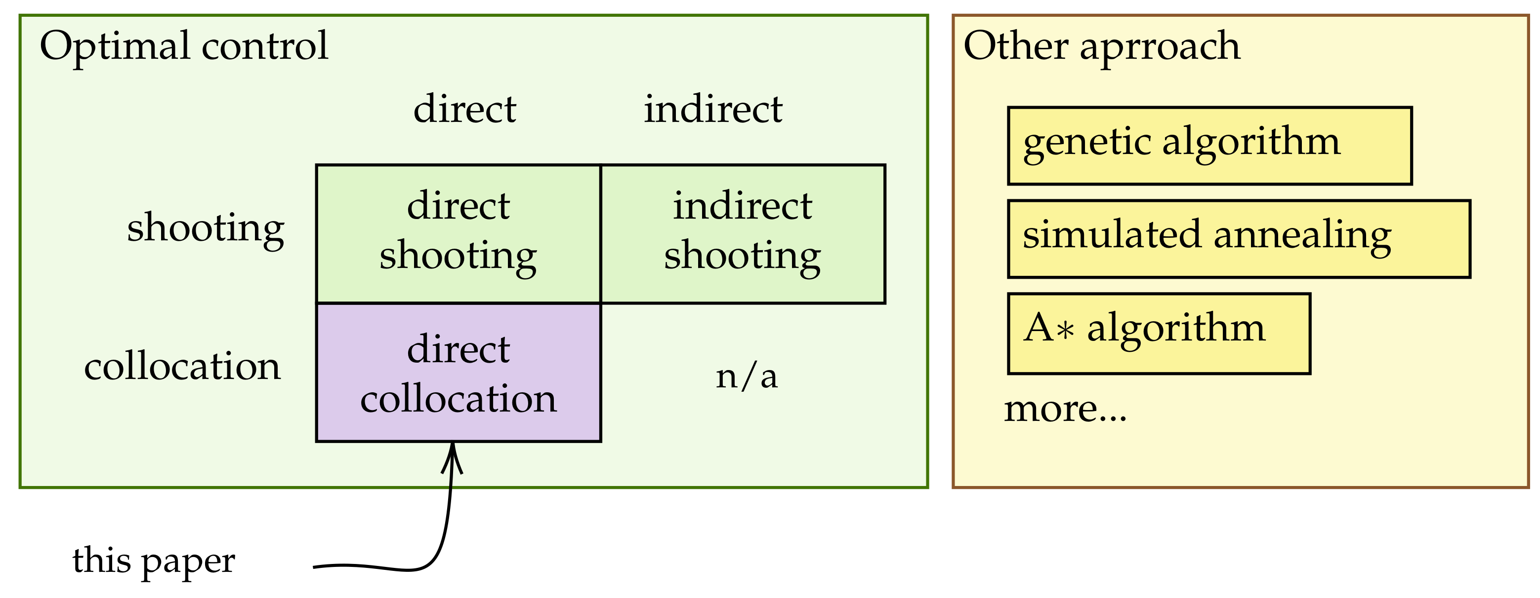
From the methodology perspective, flight trajectory optimization can be divided into two main domains [8], which are the optimal control approach and the non-optimal control approach. The non-optimal control is a general category that covers many different algorithms, including genetic algorithms [9], simulated annealing [10], and algorithm [11]. The advantage of these optimization approaches is that they are simple to set up. However, they often have to work with discretized state spaces, cannot take advantage of the system dynamics of the flight, and require a long time for the (sub-)optimal solution to be found.
The optimal control approaches take advantage of system dynamics, and they model the generations of a flight trajectory as a system with control variables (e.g., speed, vertical rate) and state variables (e.g., positions, altitude, mass). Generally speaking, the kinematic model of the aircraft provides the state equation, while the dynamic model (e.g., force, fuel, total energy) provides the constraint conditions.
Optimal control can be further divided into direct optimal control (first discretize then optimize) or indirect optimal control (first optimize then discretize) [12]. From the trajectory method perspective, it is also possible to perform optimal control using the shooting method and collocation (simultaneous) method. The shooting method parametrizes the control trajectory with a smooth piecewise approximation and includes states at certain shooting nodes as decision variables in solving the non-linear programming problem. On the other hand, the collocation method parametrizes the entire state trajectory as low-order piecewise polynomial functions and adopts all states at collocation points as decision variables. Figure 1 shows an overview of the aforementioned methods.
Overall, the direct collocation optimal control approach provides better performance for finding the optimal solution over the shooting method. It has been adopted by recent research studies [13,14]. However, of all previously mentioned optimization methods, direct collocation is the one that is the most difficult to set up, given that the constraints are closely linked with the underlying aircraft performance models. The challenge becomes more complicated when dealing with different flight phases or full trajectories. This paper addresses all these challenges.
1.2. Aircraft Performance Models and Optimization Scopes
At the center of flight trajectory optimization is the aircraft performance model, which includes the kinematic model and dynamic model of the aircraft. The kinematic model describes the motion of the trajectory, including parameters like position, altitude, speed, and vertical rates. Commonly, a simplified point-mass model is used for the dynamic model, which deals with different forces (thrust and drag), mass, and fuel burn.
Currently, the most used aircraft performance model for flight trajectory optimization is the Base of aircraft data (BADA) developed by EUROCONTROL [15]. BADA is a comprehensive model with a large number of aircraft types. However, it is also a closed-source model that requires a per-project-based license, and its utilization prevents many trajectory optimizers from being openly shared, hence, hindering the comparability, reusability, and reproducibility of follow-on research studies.
Another aircraft performance model, ECAC Doc 29, developed by the European Civil Aviation Conference, is an open model, with a focus on the impact of aircraft noise [16]. However, the ECAC Doc 29 has a low fidelity and only focuses on the noise model. External models, like BADA, are required to perform other types of optimizations.
Over the recent year, a fully open and academic aircraft performance model, OpenAP [17], has been developed as an alternative model for BADA. I have welcomed contributions from the aviation research community, and thanks to its open-source license, any parties, including academics and industries, can use this model freely. It includes the complete kinematic [18] and dynamic models required for flight trajectory optimization. Hence, OpenAP forms the basis of this paper.
Existing research studies on trajectory optimizations often have different preferences in terms of flight phases. For example, studies aiming at minimizing fuel consumption and emission often focus on the cruise segments of the flight [19,20], while others aim at the climb or descent phase of the flight [13,21,22]. Depending on the method used for optimization, lateral and vertical optimization may be performed separately, leading to a less optimal trajectory. Other factors, like wind field, can also be considered in the optimization process.
Overall, there is a lack of a generalized optimizer capable of handling all flight phases to provide a four-dimensional optimal trajectory, consider wind conditions, and uses the efficient direct collocation approach. This is the challenge set out to be solved by this paper.
1.3. Contributions of This Paper
Due to the lack of openness in the existing flight trajectory optimization libraries and their underlying aircraft performance models, reproducibility and comparability of studies remain challenges for researchers. This paper describes a fully open 4D flight trajectory optimizer, both in terms of underlying aircraft performance and emission models, as well as the implementation of optimization algorithms.
Several types of objective functions are designed and built-in with OpenAp.top. These objective models include fuel and cost index, as well as global warming potential and global temperature potential, both with 20-, 50-, and 100-year horizons. The proposed OpenAP.top [23] is one of the only open-source trajectory optimizers to date (Source code from: https://github.com/junzis/openap-top, accessed on 20 June 2022). The optimizer also provides simple interface for future research studies. Optimal trajectories can be generated with a couple of lines of code in a few seconds.
The remainder of this paper is structured as follows. Section 2 explains the aircraft performance and emission models from OpenAP, as well as the adaptions of these models for trajectory optimization from a non-linear optimal control approach. Section 3 describes the fundamentals of non-linear optimal control for general trajectory optimization. Section 4 dives into the details of designing the optimization constraints for flight trajectory optimization in the context of air traffic studies. Section 5 explains the design of different categories of objective functions. Section 6 focuses on the optimization experiments conducted under different considerations, such as with flight phase and different objectives. It also provides insightful analyses of the optimization performance under uncertainties, such as aircraft mass, cost-index setting, and wind conditions. Finally, Section 7 and Section 8 present the discussion and conclusions of this paper.
2. Aircraft Fuel and Emission Models
OpenAP is the underlying model used in this paper to calculate aircraft performance, fuel consumption, and emissions. In this section, I briefly describe the fuel and emission models, which are slightly different from the original OpenAP models.
The fuel flow model is built upon the openly available ICAO aircraft engine emission databank [24]. The ICAO data provides engine fuel flow at different thrust settings at sea-level ambient conditions. Four thrust ratios are 100%, 85%, 30%, and 7% of the maximum thrust, representing takeoff, climb out, cruise, and idle flight conditions respectively.
Based on these four testing data points, a second-order polynomial model is constructed to represent the fuel flow for different power ratios. The original third-order polynomial model from OpenAP is adapted to prevent the occurrence of negative fuel flow during optimization by the numerical solver. The model for calculating fuel flow at sea level () can be described as:
where T is the actual thrust, is the maximum thrust, and is the thrust ratio at time t, and coefficients a and b are obtained from the least-squares regression using the four testing conditions. During the flight, the data from the ICAO engine emission databank at sea-level conditions are no longer valid. In OpenAP, a correction factor is introduced to correct the altitude effect on engine flue flow. The final fuel flow model can be expressed as:
where h is the altitude of the aircraft, and is the correction coefficient that is dependent on engine types [17]. T are calculated based on the aircraft drag polar as:
where m, , v are aircraft mass, air density, and speed. Aircraft wing area (S) and drag polar coefficients ( and k) are both parts of the OpenAP aircraft performance model.
Once the fuel flow is know, different emissions are calculated. Among different emission types, H2O , CO2 , SOX , and soot are considered to be proportional [25] to the fuel flow regardless of the atmosphere conditions:
Other emissions, including NOX , CO, and HC, are first estimated based on the sea-level atmospheric conditions based on data from the ICAO engine emission databank. To simplify the model, piecewise linear interpolation models are designed to approximate emissions under different thrust conditions. After that, the Fuel Flow Method 2 developed by Boeing [26] is used to correct the emission values based on the flight altitude.
3. Non-Linear Optimal Control for Trajectory Optimization Problems
The non-linear optimal control approach applies to many trajectory optimization problems in different research areas, including robotics, unmanned vehicles, and spacecraft. In this section, I give a brief overview of how such a system is formulated for flight trajectory optimization and how to solve it numerically.
3.1. System Equations
In the point-mass aircraft performance model, the following flight states are considered:
where , h, and m are the position, altitude, and mass of the aircraft. The 2D positions can be conveniently converted from and to latitudes and longitudes based on map projections [27]. In the framework of OpenAP.top, the Lambert Conformal Conic projection and World Geodetic System (WGS) 1984 [28] is used for such conversions.
For this point-mass system, the control states includes:
where M, , and are Mach number, vertical rate, and heading of the aircraft. These states correspond to the parameters that can be set by the flight management system of the aircraft.
The dynamic, or evolution, of the states can be expressed by a set of ordinary differential equations:
where v is the true airspeed, is the flight path angle, and is the fuel flow model that is dependent on the aircraft mass, speed, and altitude. and are wind speed components. Other intermediate variables such as flight path angle and true airspeed are calculated based on Mach number and altitude under the international standard atmosphere conditions:
where is the speed of sound constant at sea level, is the ratio of specific heat, R is the gas constant for air, and is the air temperature at altitude h.
3.2. Non-Linear Optimal Control
Knowing states, controls, and the dynamic of an optimal control system, the next task is to formulate it in a way that can be solved by non-linear programming that consists of a set of constraints and an objective function. The generalized form of an objective function (J) can be expressed as:
where and are the Mayer term and Lagrangian terms. They correspond to the cost at the endpoints, as well as cost along the trajectory, respectively. The minimization of the objective function
is subject to the following constraints:
where is the first-order dynamic constraint represented by the earlier system equations, represents the path constraints, and represents the conditions at endpoints.
3.3. Numerical Approximations
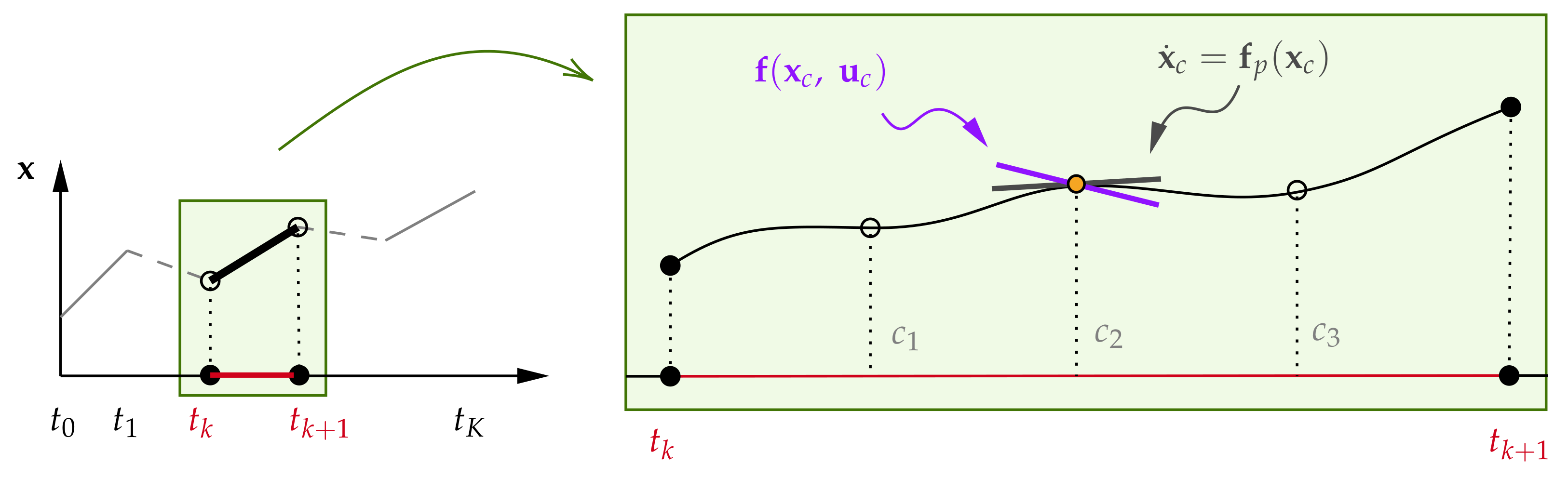
The solution for such an optimal control problem can be computed numerically. The direct collocation approach adopted in this paper discretizes the continuous problem into segments that consist of K number of time intervals. Within each interval, the states are approximated using polynomials at collocation points in each time interval. Such a discretized system has the following form of objective objectives:
where refers to the set that contains the last collocation points of each interval. is the time between collocation points. The minimization of the objective is subject to the following conditions:
The final cost is obtained by integrating the cost at all collocation points for all intervals:
With in each time interval, states at these collocation points are also evaluated with the following constraint:
where is the state dynamic approximated by the lagrange polynomial ():
3.4. Solver
Since the trajectory optimization problem is formulated as a discretized non-linear programming problem, a numeric solver can be employed to derive the optimal control states (and related flight states). The numerical solver used in this paper is implemented by an open-source library CasADi [12], which is a symbolic framework for numeric optimization and automatic differentiation. CasADi further utilizes the lower-level C code that invokes the Interior Point Optimizer (IPOPT) [29] to solve the non-linear programming problem.
4. Flight Trajectory Optimization Constraints
One of the most challenging tasks is to identify correct constraint models at different stages of the flight and link the aircraft performance constraints with all control nodes and collocation points. This section dives into the details of how the constraints are crafted for different scopes of the flight, including complete trajectory, multiphase trajectory, cruise trajectory, climb trajectory, and descent trajectory.
4.1. Complete Flight Trajectory
The goal of a single optimal complete trajectory is to generate the global 4D flight from the initial climb to the final approach. Flight phases are not explicitly expressed, which implies that the optimizer needs to generate the optimal climb, cruise, and descent automatically from the origin to the destination, considering the performance limit of the aircraft and wind conditions at different locations and altitudes.
4.1.1. Endpoint Constrains
The endpoint constraints of Equation (24) consist of:
which stipulates that starting and ending positions are the locations of the departure and arrival airport. The initial mass is specified as the aircraft takeoff mass (). The landing weight is between the operational empty weight and the maximum landing weight. The minimum altitude () is 3000 feet in OpenAP.
4.1.2. Path Constrains for States
The path constraints of Equation (23) includes the following constraints on state variables and control variables:
It is worth noting that an additional 10 km is added to the lateral boundaries for handling the case where the origin and destination have the same latitude or longitude. Otherwise, the boundary becomes a line instead of a square.
4.1.3. Path Constraints for Aircraft Performance
The first performance constraint represents the relationship between thrust and drag. At each interval, the maximum thrust available must be greater than the total drag of the aircraft. This constraint can be expressed as:
where represents the maximum thrust model of the aircraft at different altitude and speed conditions. and k are drag polar coefficients, S is the wing area, and is the air density under ISA conditions.
The second performance constraint is to prevent stalls of the aircraft. Hence, the maximum lift should always be higher than the weight of the aircraft. These constraints are:
where is the maximum lift coefficient.
The third performance constraint defines the total energy changes. This is to ensure the available excess power of the engine can cope with the required increase of the aircraft’s kinetic and potential energy. This constraint can be formulated as:
All model coefficients for thrust, drag polar, and aircraft properties are part of the underlying OpenAP, and, in addition, the default value for the maximum lift coefficients is empirically set to 1.4.
4.1.4. Path Constrains for Smooth Control Variable Changes
In addition to the previous constraints, I consider a set of additional constraints to ensure limited variabilities in control variables. The following equations describe the allowed variations among a sequence of control variables
Previously, vertical rate covers the entire performance envelope. To further eliminate possible corner cases of large en-route vertical rate changes, the following constraint is applied to the intervals that are (presumably) part of the cruise flight:
where is determined by the OpenAP kinematic model. The set includes the points beyond the maximum climb range and before the start of the maximum descent range.
4.2. Cruise-Only Flight Trajectory
For optimization focused only on the cruise phase of the flight, several adaptions to constraints are proposed. First of all, the endpoint constraints for the flights at the cruise phase are:
indicating that the starting and ending positions are the top of the climb and the top of descent. Additionally, the initial mass is the aircraft mass at the top of the climb.
The following adaptation is made to the path constraints for state and control variables, including altitude, Mach number, and vertical rate:
4.2.1. Additional (Optional) Constrains for Cruise Flight
Several optional constraints are made available for cruise flights, for example, to limit the flight with a constant altitude, fly at a constant Mach number, or allow the execution of descent during the cruise. The constant altitude imposes the following constraint:
Similarly, the constant Mach number imposes the following constraint:
When descent is allowed during cruise, the constrain in Equation (36) is changed to:
which enables aircraft to seek a lower altitude during the cruise for flying at more optimal conditions. Note that this type of maneuver is not used in current flight operations. However, such a relaxation of the constraints allows the optimizer to seek, for example, a lower altitude with more optimal wind or contrail conditions.
4.3. Climb-Only Flight Trajectory
When a specific study focuses on the climb phase of the flight, adaptions can also be made to the constraints to provide more accurate climbing trajectories.
The endpoint constraints for climbing flights are:
which specifies that starting as the origin airport. The initial mass is the aircraft’s takeoff mass.
The challenge in optimizing the climbing trajectory is that one cannot know the endpoint before the optimization. For example, both the optimal cruise altitude and the range of climbing are not known in advance. Hence, the cruise optimizer is performed first to obtain a pseudo-optimal cruise altitude. A fixed flight range (larger than the maximum climbing range) is chosen to provide the same basis for evaluating the fuel and time cost. The endpoint constraints are defined as:
where is the maximum climb distance based on the OpenAP kinematic model. is the optimal cruise altitude obtained with a pre-run of the cruise optimizer. Equation (61) ensures that the final position is aligned with the optimal cruise trajectory, where (, ) represents the second interval point in the cruise phase.
For other state and control variables, the following adaptations to path constraints are applied to the optimizer:
4.4. Descent-Only Flight Trajectory
Similarly, as for climbing flights, specific constraints can also be designed to generate descent-only trajectories. The same pseudo-optimal cruise trajectory is used since the top of the descent is generally not known before the optimization. The endpoint constraints for descent flights are:
which specifies the end of the trajectory at the destination airport. The initial mass is approximately the aircraft mass at the end of the cruise. Similar to the previous climbing optimization, the determination of the top of the descent can be a challenge. Hence, additional constraints are designed for identifying the top of the descent.
where is the end of the psuedo-optimal cruise altitude. Equation (69) ensures the starting position is align with the optimal cruise trajectory, where (, ) is the second last interval point of the cruise trajectory.
For other state and control variables, the following adaptations to path constraints are applied to the optimizer:
In addition, the following constraints represent the forces acting on aircraft and ensure the equilibrium among weight, idle thrust, and drag:
where is the flight path angle, which is a negative value during the descent. Idle thrust can be calculated based on the OpenAP model, which is assumed to be approximately 7% of the maximum thrust at the given altitude and speed.
4.5. Multiphase Complete Trajectory
The approach in Section 4.1 can generate a globally optimized complete flight trajectory. Since the nodes are designed to be equally distributed along the time dimension, for longer flights, we need to use a large number of nodes to sufficiently cover the climb and descent phases in detail. This can add unnecessary computational time for the long cruise phase. In this case, a multiphase complete trajectory can be generated by combining previous optimal climb, cruise, and descent trajectories separately.
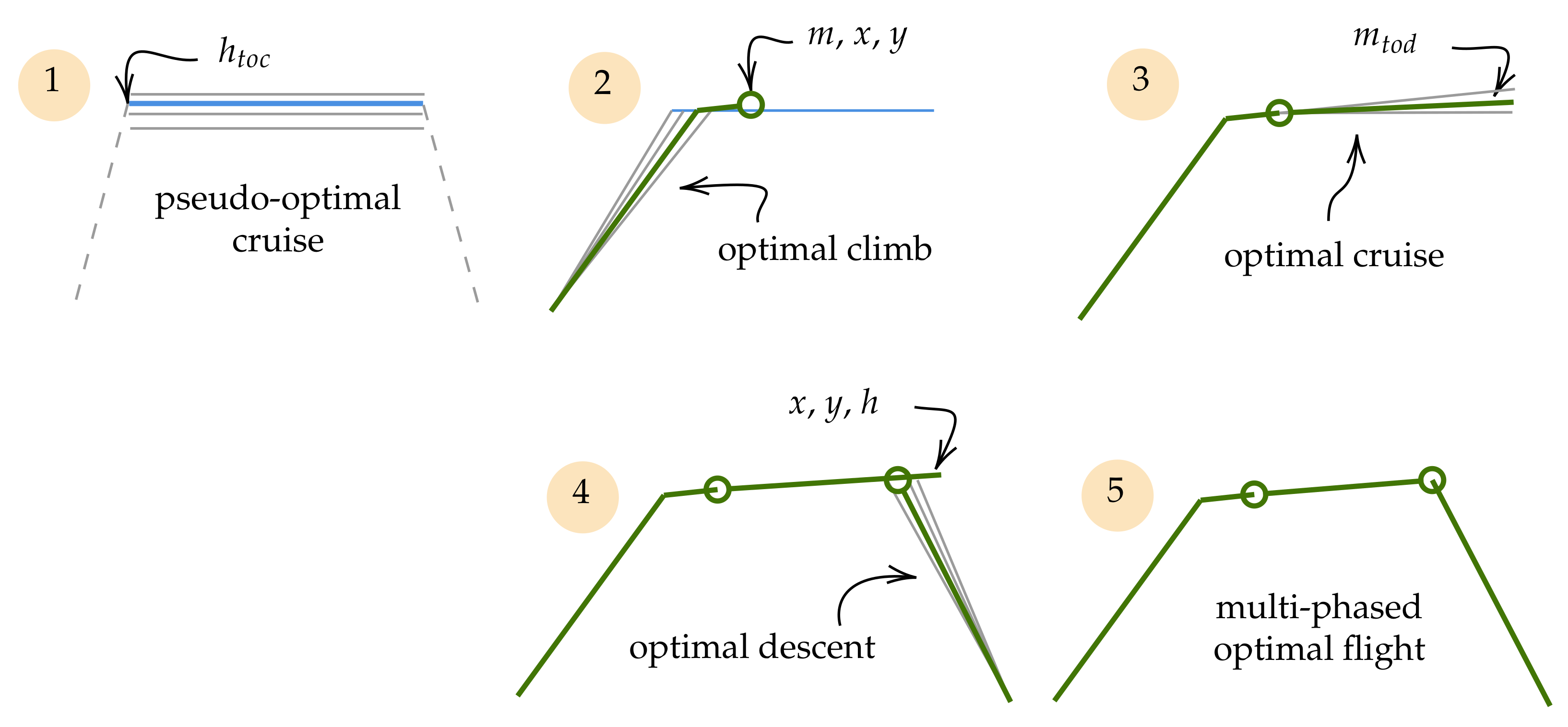
The main challenge is to have a consistent top of climb between climb trajectory and cruise trajectory, as well as a consistent top of descent between cruise and descent trajectory, considering the same objective functions for all separate flight phases. In Figure 3, the steps for constructing the entire multiphase optimal trajectory are shown.
First, the top of climb altitude is found based on the pseudo-optimal cruise trajectory. The optimal climb is generated based on this final altitude. After that, the actual optimal cruise trajectory is obtained based on the final location and mass of the climbing trajectory. The optional descent trajectory is also found based on the altitude and position at the end of the cruise. Finally, the complete trajectory is obtained from the intersection of all phase segments.
It is worth noting that in the multiphase approach, the top of climb altitude may differ from the actual optimal top of climb altitude, which should be higher due to fuel consumption during the climb. However, the flight continues to climb during the follow-on cruise phase and to search for optimal altitude.
5. Objective Functions
The second main area of research in the paper is objective function models. Conventional objectives are designed to optimize flights for fuel and time. In addition, objectives reflecting the environmental impact of flights are also implemented.
5.1. Optimizing for Fuel Consumption
The default optimal trajectory is the one that is optimized for the total fuel consumption. The Lagrangian term in Equation (21) is the fuel consumption between collocation points:
where is the fuel flow estimated at the collocation points.
5.2. Optimizing for Flight Time
It is also possible to optimize the trajectory to minimize the total flight time. The Lagrangian term is then simply:
5.3. Optimizing for Cost Index
In current flight operations, trade-offs are made between fuel and time. Aircraft operators can optimize the trajectory that has a specific balance between the fuel consumption and flight time, which is modeled as cost index [2,3]. The cost index model is comprised of a range of numbers, where a lower number considers fuel cost more importantly, while a higher cost index number values more the flight time. Different aircraft manufacturers use different ranges of cost indexes.
In OpenAP, the cost index range is between 0 and 100. The objective term for the trajectory Optimizer is formulated as:
where is the cost index, and and are costs for time and fuel, which can the specified as input parameters. The default costs used in OpenAP are:
where the default time cost is similar to [2], while the fuel cost is approximately the price during the year 2021 in Europe. Note that these coefficients are simplifications and can be adapted.
5.4. Minizing Global Warming and Temperature Potential
Aviation sustainability research deals with flight emissions and their climate impacts. Different emissions have distinct impacts on the climate due to their ability to absorb energy (radiative efficiency) and the lifetime of these gases [30].
In this paper, two sets of models, global warming potential (GWP) and global temperature potential (GTP), is used for the optimization of the trajectories based on research in [30]. GWP models energy absorbed by different gases compared to the energy absorbed by the same amount of CO2 at different time horizons (20, 50, and 100 years), while GTP models the temperature change at the end of these different periods.
6. Experiments
In this section, I conducted several sets of experiments to demonstrate the capability of the proposed trajectory optimizer. First of all, example trajectories are generated to showcase the generation of full and partial 4D trajectories under realistic wind scenarios. Then, I focus on the analysis of how different objectives affect the different climate metrics of the flight, aiming at quantifying the relationships among different climate objectives. The final set of experiments focuses on understanding the differences in optimal trajectories that are linked to uncertainties in aircraft performance parameters, such as different initial mass, selection of cost index, engine differences, and varying wind conditions.
6.1. Single Trajectory and Flight Phases Optimizations
The demonstration of single optimal trajectory generation creates a set of trajectories between Amsterdam Airport Schiphol (EHAM) and Athens International Airport (LGAV). At first, the optimal complete trajectories including all flight phases are created using the two different approaches (complete and multiphase) proposed earlier. Then, optimal trajectories at each flight phase are generated.
For all trajectories in this set of experiments, the objectives are total fuel consumption. Airbus A320 is chosen as the aircraft type carrying the flights, and all flights are all initialized with 85% of maximum takeoff mass (approximately 66 metric tons). For most of the tests, wind data of 08:00 on 1 May 2021 from the ERA5 reanalysis dataset are used, which was obtained from the European Centre for Medium-Range Weather Forecasts datasets.
6.1.1. Optimization of the Entire Trajectory
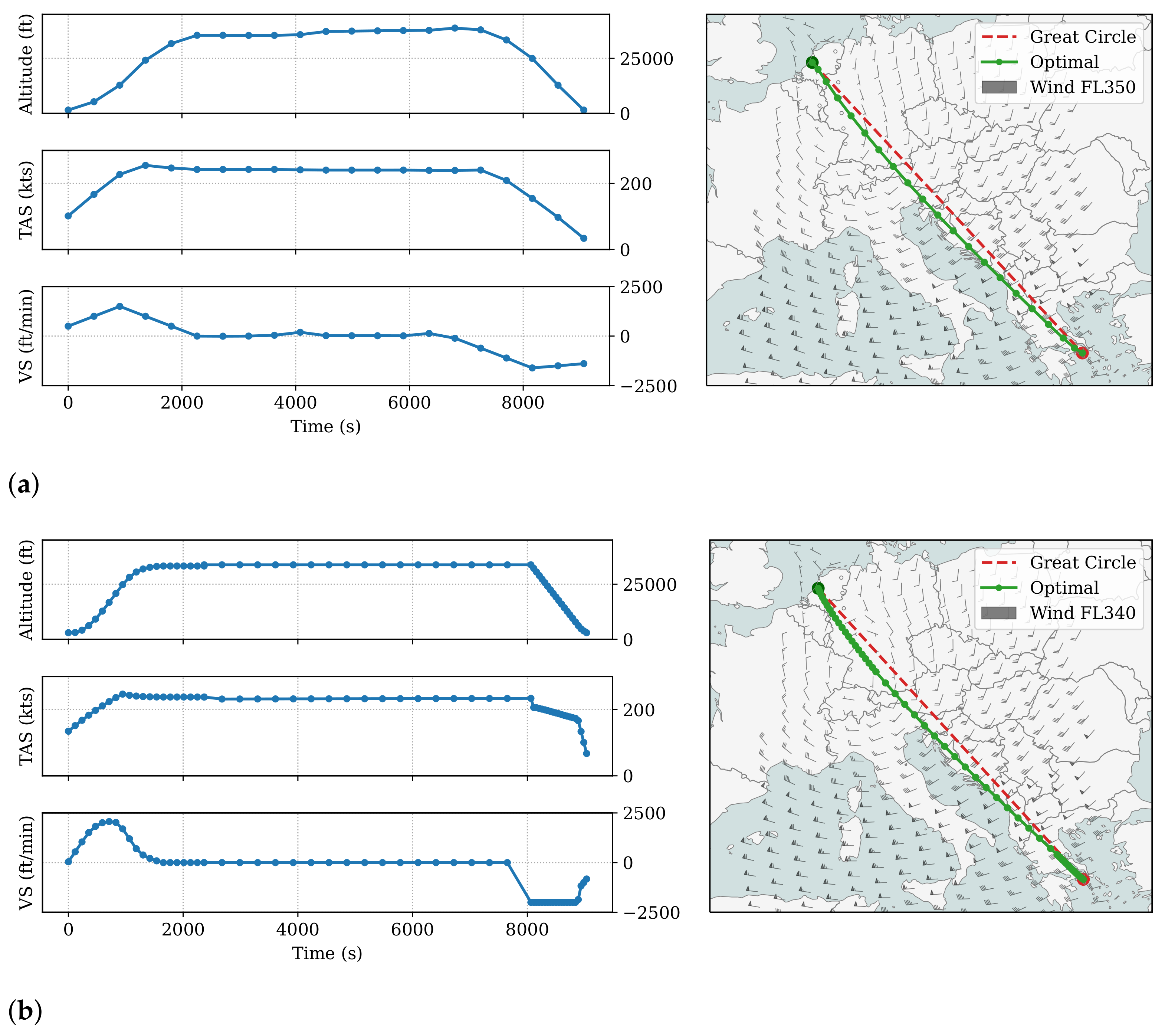
In Figure 4, the complete and multiphase optimal trajectories are shown. Overall, the two trajectories have similar flight profiles and lateral trajectories. The main difference is the varying resolution at different flight phases in the latter approach, which provides more accurate climb and descent trajectories.
However, the multiphase approach does not always yield the optimal complete trajectory. This can be seen by inspecting the top of the descent for both trajectories. The multiphase trajectory shows a discontinuity in speed, with indicates that a lower final speed (hence higher altitude and earlier top of descent) would be more optimal. This is what the complete optimal trajectory can provide, as shown in the first set of plots.
6.1.2. Optimization of Different Flight Phases
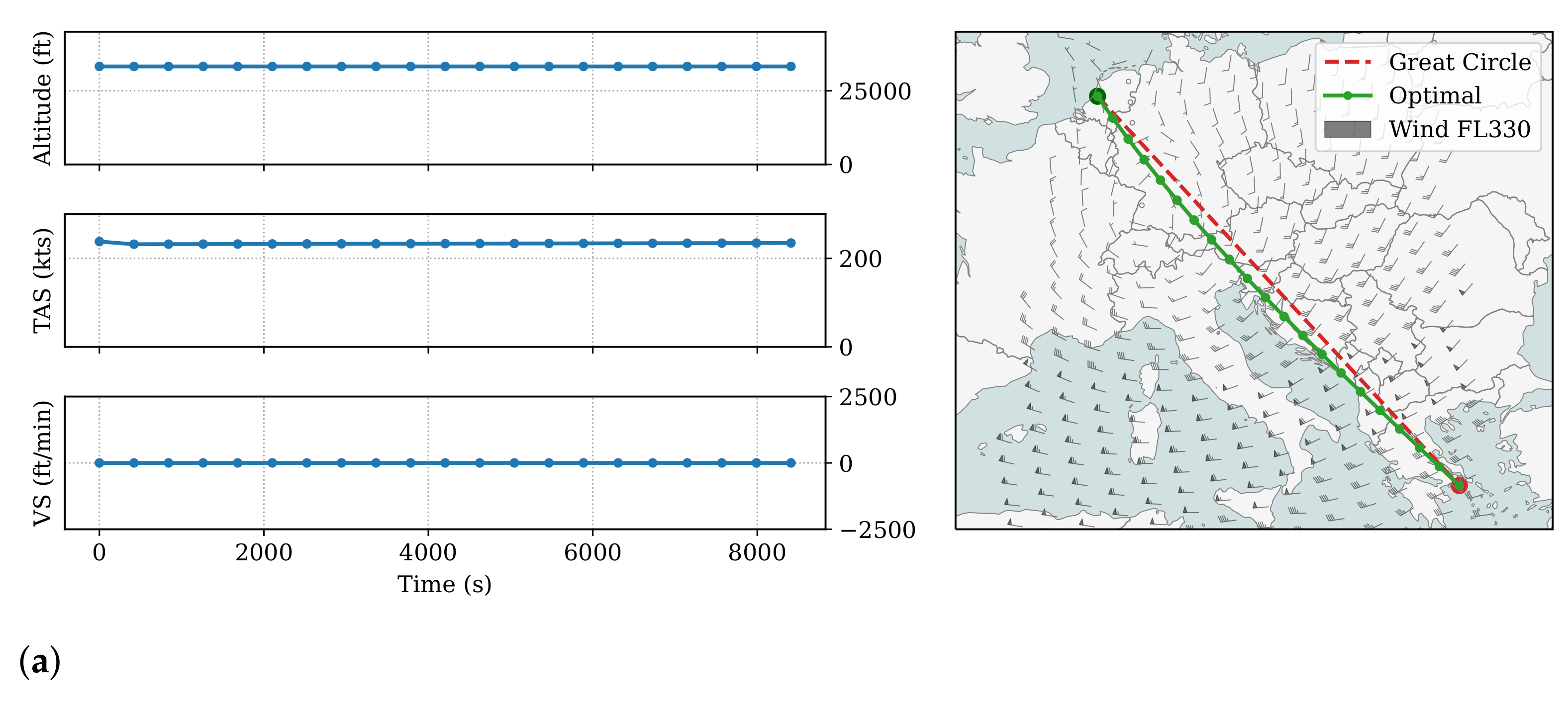
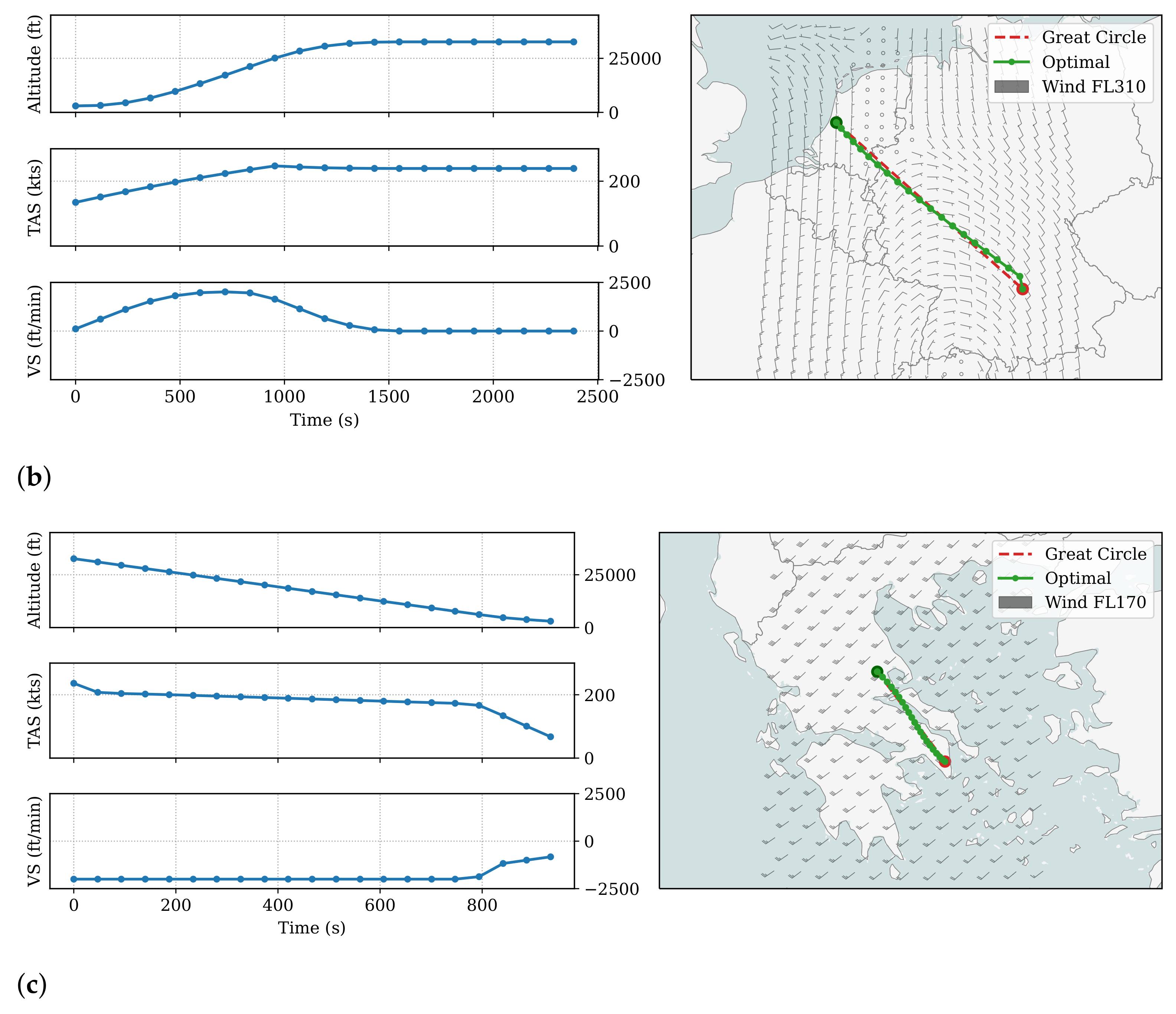
Figure 5 illustrates the climb, cruise, and descent trajectories. Essentially, these are the base segments that constructed the earlier multiphase full trajectory with the method described in Section 4.5.
For the cruise trajectory in Figure 5a, the selected optimal altitude is at approximately 33,000 ft, and the speed is determined to be around Mach 0.78. The optimized trajectory deviates from the great circle flight path at the start and takes advantage of tailwind (components) during the later stages of the flight. It is worth noting that the origin and destination are set at departure and arrival airports. However, the positions can be any coordinate in the OpenAP.top cruise optimizer.
The climb trajectory first identifies the altitude and bearing at the top of the climb, based on the earlier pseudo-optimal cruise trajectory. The climb optimization aims at the most fuel-efficient 4D path (considering the wind) that reaches the desired altitude and final bearing. Since the wind dynamic can be quite different at a lower altitude, a small discrepancy may occur between positions of the actual top of climb and cruise, which is shown in the final point of Figure 5b. Due to the formulation of the climb optimizer that employs an aircraft type code-specific range parameter, the generated trajectory usually consists of both climb and a small segment of the cruise. To obtain only the climb phase, one can simply remove the final segment where the vertical rates are close to zero.
Figure 5c illustrates the descent trajectory to LGAV. The optimal vertical phase follows a continuous descent approach, where the top of descent altitude and bearing is obtained for the final segment of the cruise. It is worth noting that the point mass model and the quadratic drag polar, commonly used in air transport studies, are quite limited in modeling the dynamics of the descent. The descent segment suffers the largest uncertainties due to the inaccurate idle thrust models, as well as the lack of pitch angle-dependent lift and drag coefficient models.
6.2. Objective Metric
In Section 5, I have formulated various objective functions that can be used to produce optimal trajectories. They include fuel, time, and cost index-based conventional objectives, as well as objective models based on climate metrics like global warming potential and global temperature potential. Relationships between these objectives exist, including ones that are negatively correlated, like fuel and time, and ones that are positively correlated, like fuel and global warming potential.
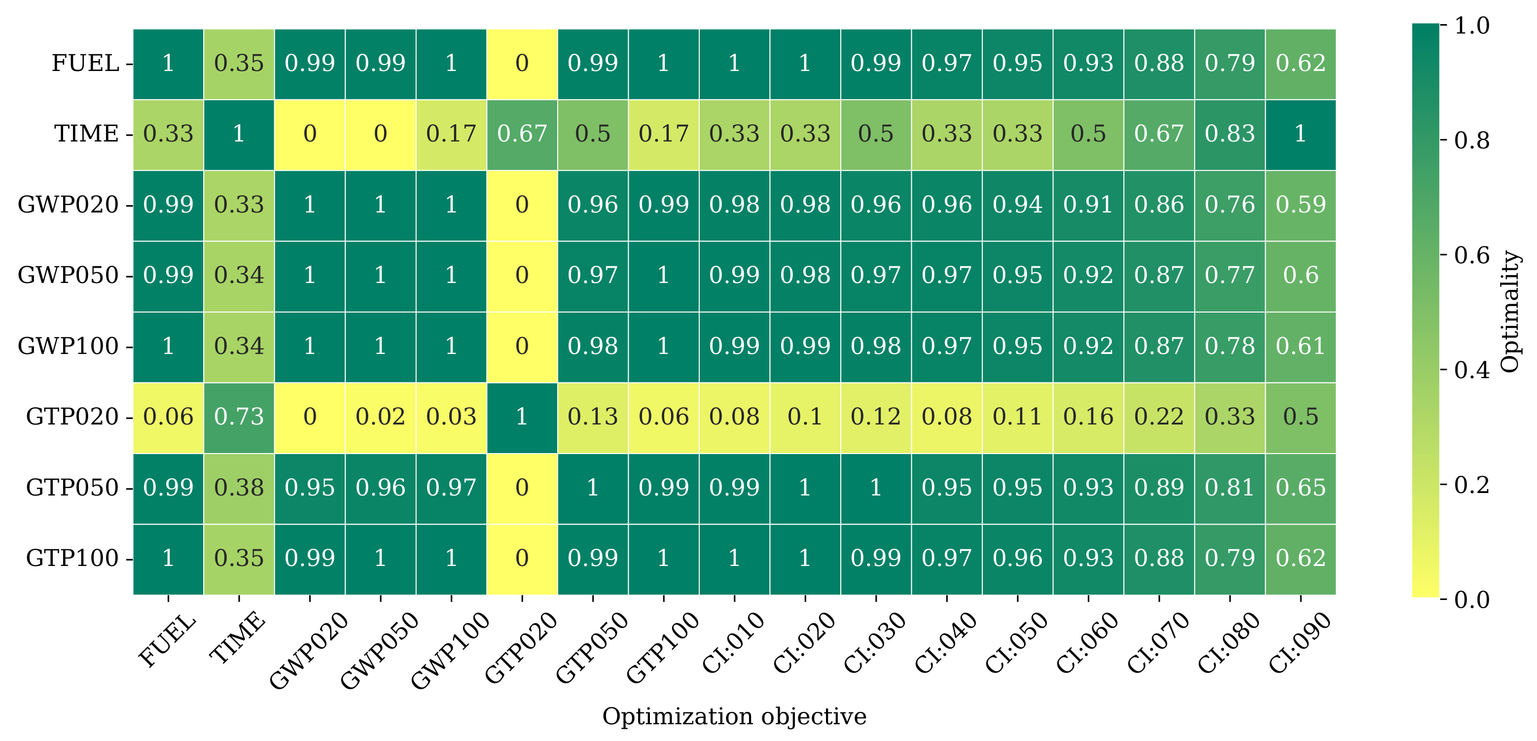
To form a clear and simple comparison of the differences between various objective functions, I design the following set of experiments, which generates multiple optimal cruising flights under all objectives, including fuel, time, GWP, GTP, and various cost indexes. Different costs (of the objectives) are also calculated for each trajectory. Each cost is normalized among all trajectories to the range of [0, 1], where 1 indicates two objectives are almost identical in cost, and 0 indicates the two objectives generate trajectories with the largest difference in cost.
The calculation of the normalized cost is:
where C is the set of costs from all trajectories on a specific objective (such as fuel, time, or GWP). For example, if one wants to evaluate how similar the GWP50 optimality is to fuel optimality. The trajectory optimized for GWP50 consumes 6.05 tons of fuel, the other flights, optimized for different objective functions, have the highest fuel consumption of 10 tons (optimized for GTP20) and the lowest of 6 tons (optimized for fuel). The score is:
which is very close to 1, meaning that optimizing for GWP50 is almost equivalent to optimizing for fuel.
Figure 6 shows the overview of these experiments. All trajectories are optimized using the same aircraft type (A320), the same initial mass (90% maximum takeoff mass, approximately 70 metric tons), the same origin and destination, and without considering the wind.
Based on Figure 6, we can see that optimizing the trajectory for all GWP metrics (20, 50, 100) and two of the GTP metrics (50 and 100) is essentially the same as optimizing for fuel consumption. This is because these metrics are dominated by the large prepositional of CO2 compared to other emissions. Since CO2 has a linear correlation to fuel consumption, these objectives are essentially the same as minimizing fuel consumption.
The only discrepancy is between the objectives of fuel and GTP20. Based on Table 2, NOX and SOX have a very large negative effect when contributing to the temperature potential at 20-year horizon. When minimizing GTP20, the optimizer yields trajectories that produce as much NOX and SOX as possible, which translates to greater fuel consumption.
6.3. Uncertainties
The following sets of experiments focus on understanding the variation of optimal trajectories under different uncertainties, specifically, considering the initial mass, engine, cost index, and wind.
6.3.1. The Influences of Takeoff Mass
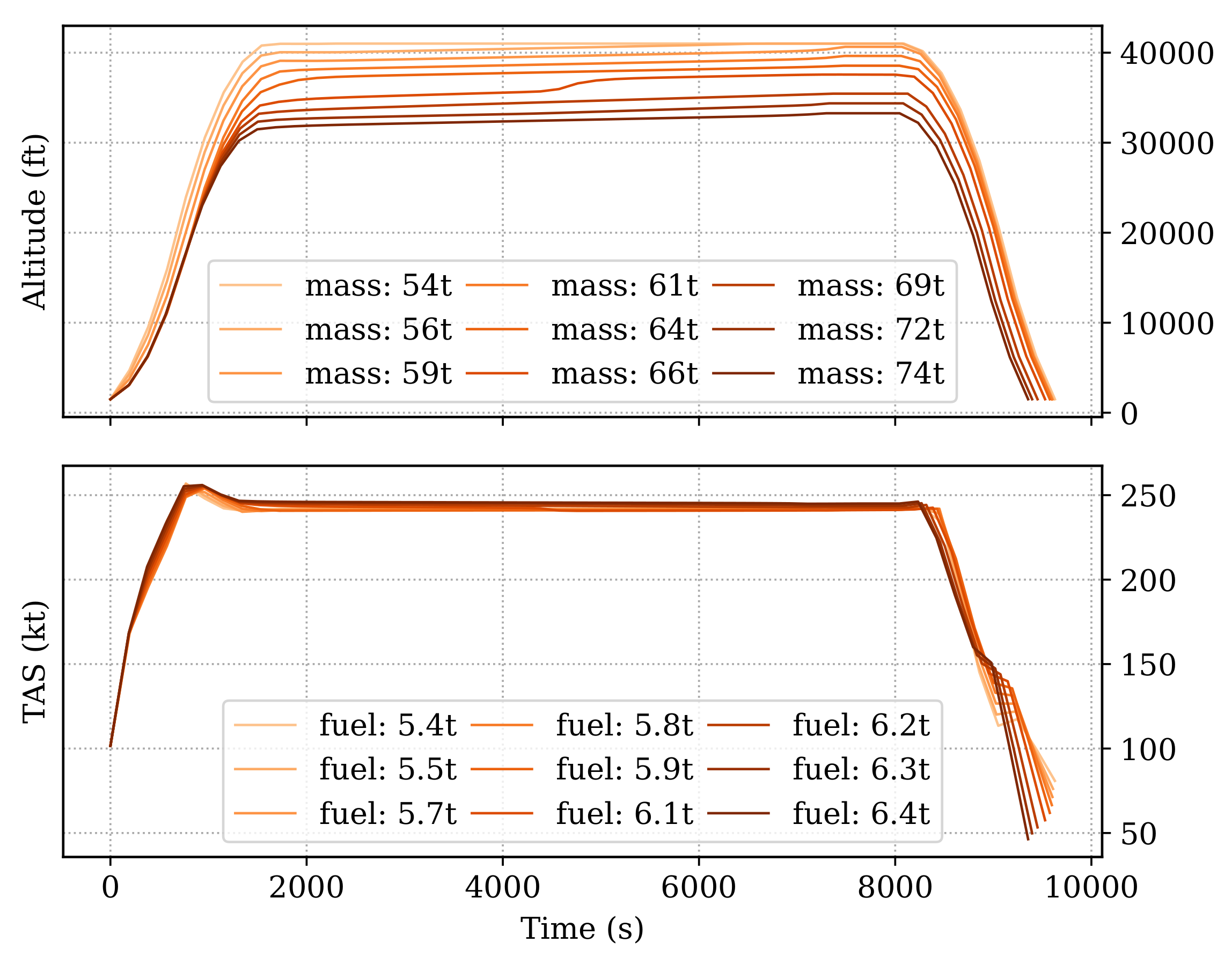
It is well known that the takeoff mass of the aircraft has a significant effect on the optimal trajectory under the same optimization objectives. This experiment aims at generating the most fuel-optimal complete trajectories under different takeoff masses of the A320 aircraft. Figure 7 shows the vertical profile.
It is possible to observe that the lighter initial mass leads to a higher altitude. The cruise altitude also increases during the flight with the decreasing mass due to flow consumption during the cruise. Such change is more apparent for heavier aircraft, where step climbs occur during the cruise.
6.3.2. Effects of Engine Configurations
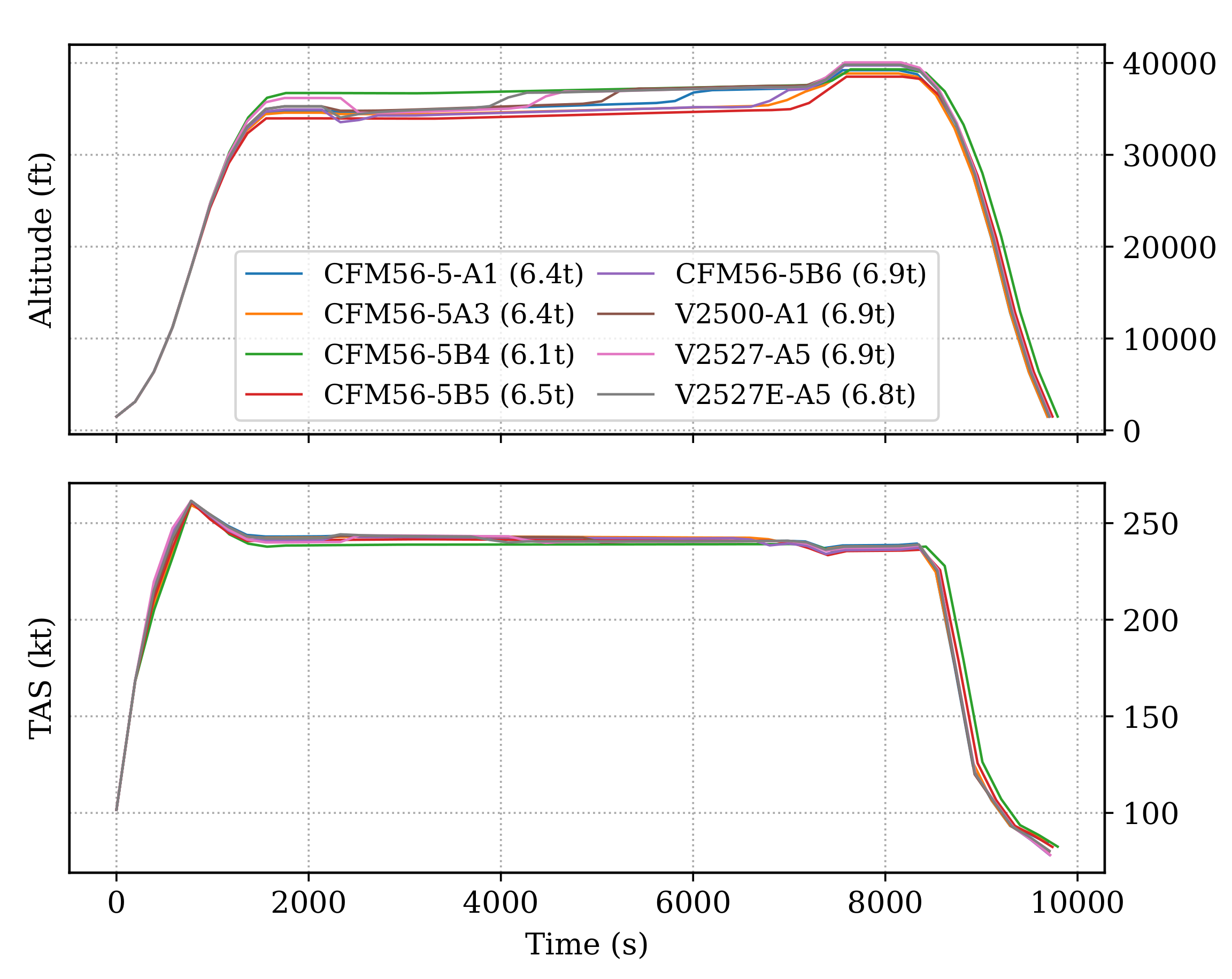
Naturally, the engine performance also affects the optimal trajectories, specifically, in terms of performance limit and fuel consumption. OpenAP.top allows for the convenient reconfiguration of engine types before the generation of an optimal trajectory. Figure 8 shows the different resulting trajectories.
Upon close inspection, a slight decrease in altitude can be observed at the start of the cruise trajectories for V2527 engines. This is likely caused by the uncertainty or inaccuracy of the maximum thrust model for these engines in the OpenAP model.
6.3.3. Simple Analysis of Cost Index
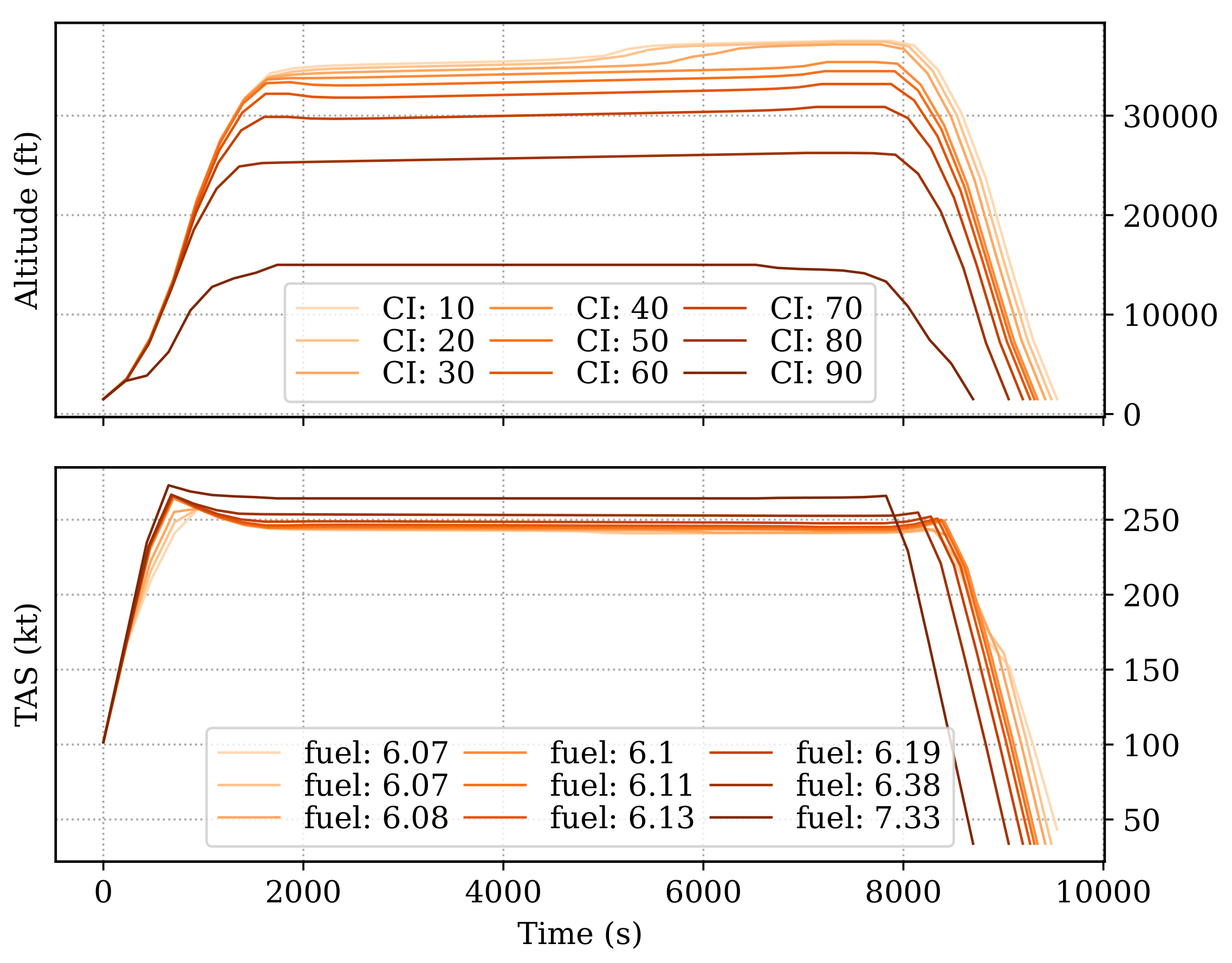
Earlier, Figure 6 shows the relationship between different metrics. The cost index changes cause the most variations. Figure 9 shows the different trajectories under the objective of varying the cost index from 10 to 90.
The experiment resulted in different fuel consumption shown in the second plot. The decrease in flight duration can be seen by the total flight time of each trajectory, with an increasing cost index value.
6.3.4. Comprehensive Analysis of Initial Mass and Cost Index Optimality
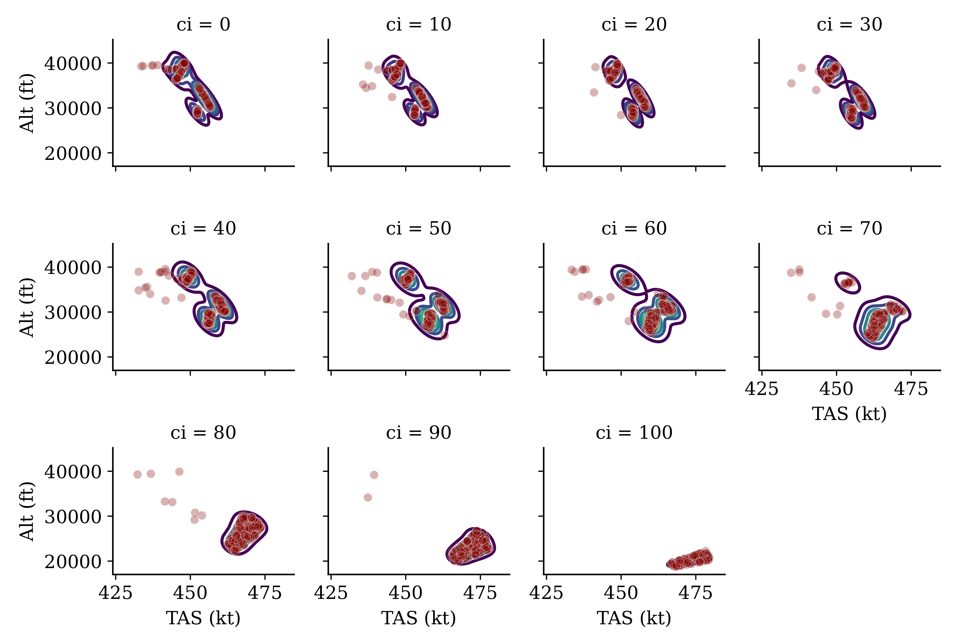
Based on the previous experiments in this section, mass and cost index are two factors that cause large variations in optimal trajectory. To test the robustness of the optimizer, I have performed a Monte-Carlo experiment, where a large sample of aircraft mass and cost indexes are sampled from two independent unformed distributions. The cost index ranges from 0 to 100, while the mass ranges from 65% to 100% of the maximum mass. In total, 2000 optimal trajectories are generated from 2000 sets of randomly sampled parameters.
I still follow the previous scenario where only cruise trajectories are generated with the A320 aircraft type without the influence of wind. I further impose the extra constraints from Section 4.2.1, which are fixed cruise altitude and fixed Mach number. This way, it is possible to study the distribution of optimal cruise altitude and Mach number, and their relationships with different initial mass conditions and objectives.
In Figure 10, I illustrate the distribution of optimal altitude and Mach number, which is grouped by different cost indexes. It can be seen that with higher cost indexes, the aircraft flies at overall lower altitudes with higher speeds, which is very consistent with operational practices. When the cost index is low, the optimal flights have a higher altitude and lower speed, which are dependent on the actual initial masses.
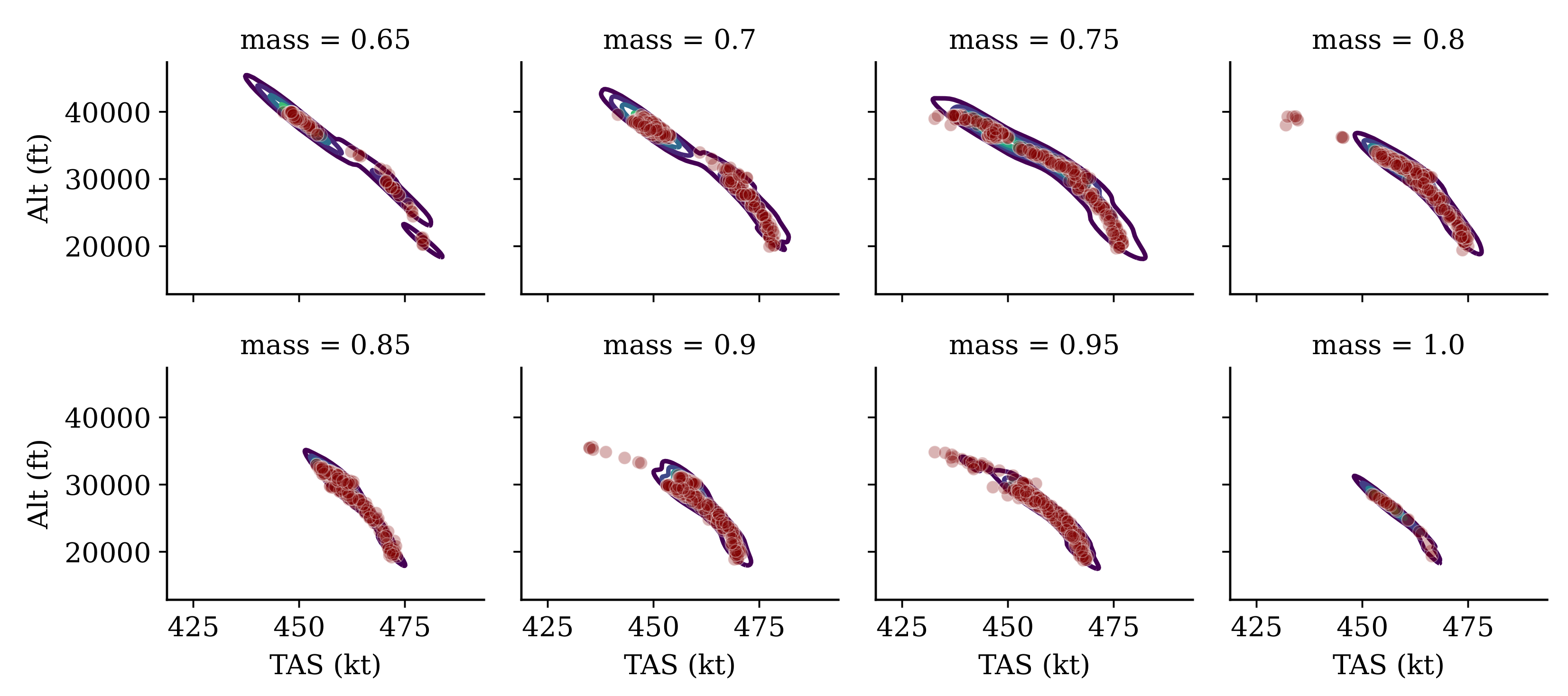
In Figure 11, the same dataset is presented and grouped by the initial mass. It is possible to see a clear negative correlation between altitude and speed under different cost indexes. With a lower mass, a large range of altitudes and speed choices are available (depending on the cost indexes). However, when the initial mass is large, the aircraft’s performance limits the freedom to select the cruise altitude and speed.
6.3.5. Effects of Varying Wind Conditions
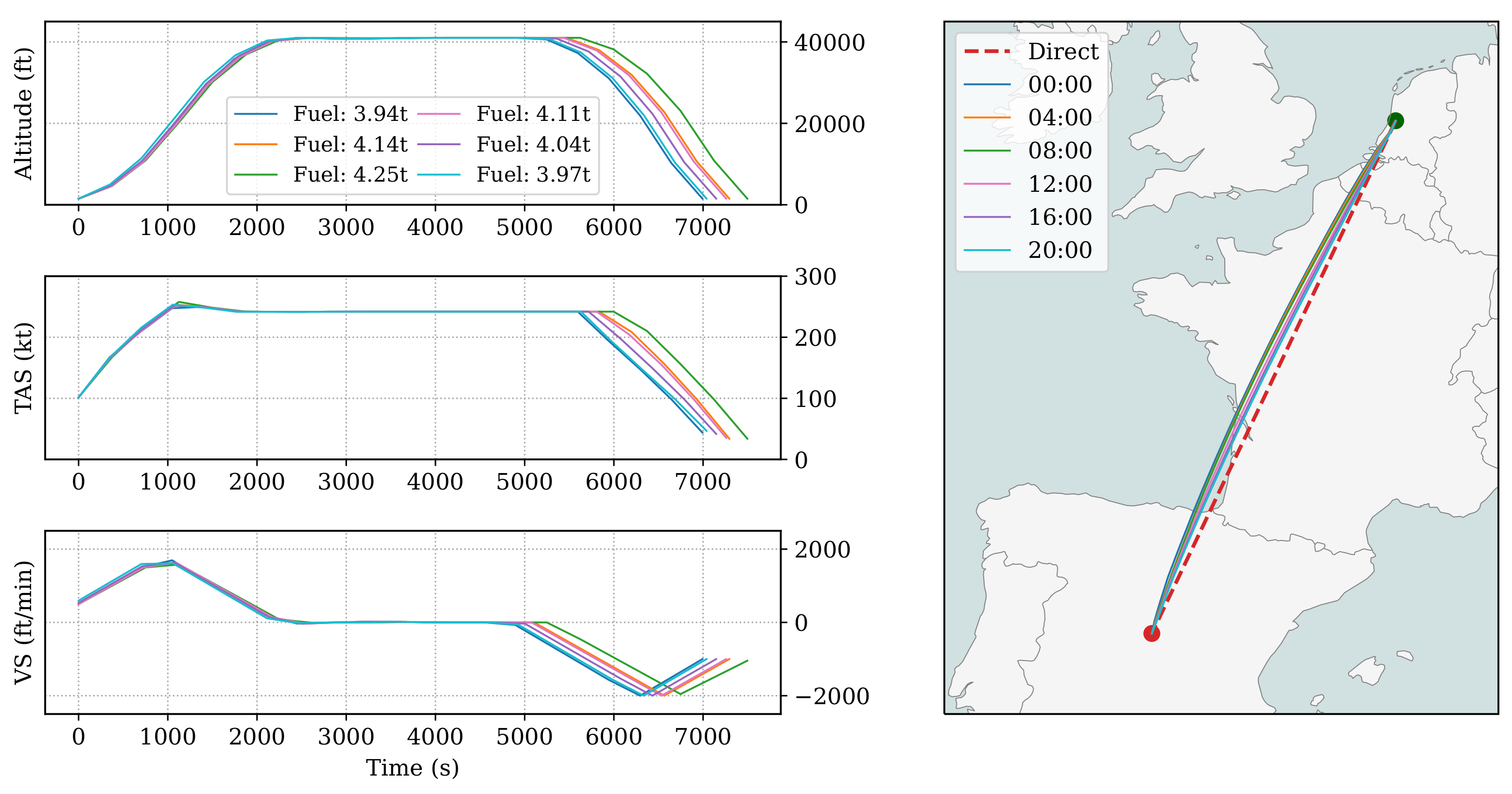
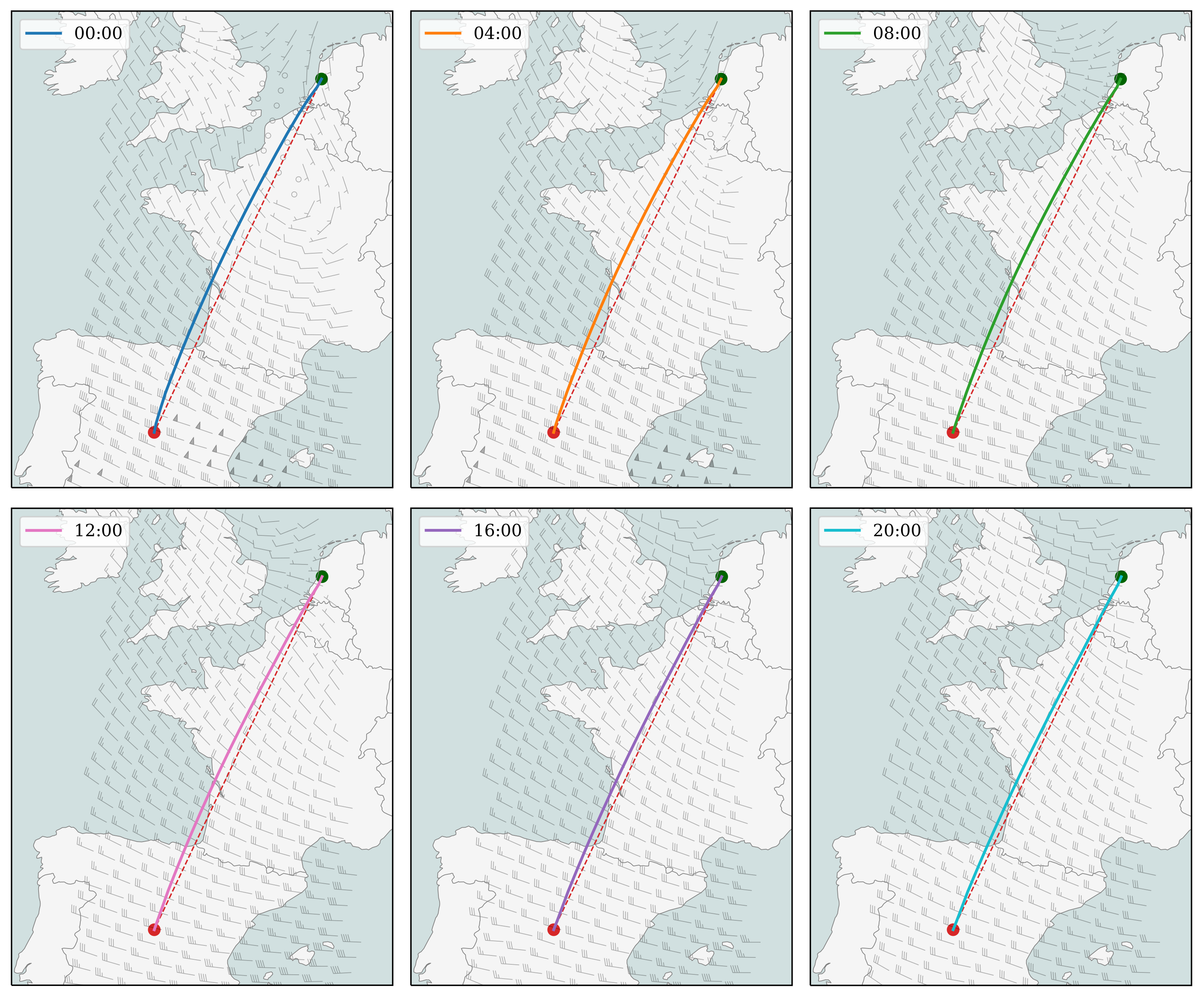
The final set of experiments demonstrates how flight trajectory adapts to the varying wind conditions during daily operations using the proposed optimizer. First, I obtain a dataset that consists of wind fields for May 1, 2020, from the ERA5 data repository. The dataset contains the wind field of every 4th-hour segment. Six optimal trajectories are generated with the same origin and destination, as shown in Figure 12.
Overall, the vertical profiles are similar except for the cruise durations. The relationship between lateral deviations and wind conditions during the day can be observed. Figure 13 illustrates the trajectory and the wind field used for optimization.
It is possible to see that during the early hours, the optimizer can take advantage of the tailwind component during the second half of the flight, where it deviates from the shortest distance by achieving greater fuel optimality. In addition, due to the advantage of the tailwind, the flight time is also the shortest for the first wind scenario.
7. Discussion
In this section, I further elaborate on the proposed open flight optimizer, OpenAP.top, and reflect on some of the earlier experiment results, explain the limitations, and propose the further evolution of this flight optimizer.
7.1. Insights into the Optimal Control Flight Optimization
The survey [8] suggests that even though the optimal control is more reliable and robust than the non-optimal control approach (e.g., metaheuristic), the drawbacks in implementation complexity have prevented its widespread usage. Successful implementation requires a deep understanding of aircraft performance models, mathematical optimization, and programming knowledge. The main challenge of this study is to combine all three of these different domains to produce results.
Another challenge is to design the proper constraints that allow the optimal complete trajectory to be generated. Such a trajectory requires careful consideration of aircraft performance models and performance limits. A large part of this paper, Section 4, explains the details of how these constraints are designed for different flight phases. To overcome unrealistic exceptions, part of the OpenAP is redesigned. For example, the fuel function is changed to avoid negative values produced outside of the aircraft performance thrust boundary.
The underlying optimization libraries, CasADi and IPOPT, require a lot of practice and tuning to formulate and solve the flight trajectory optimization problem. Because the python code is converted into C code by CasADi for IPOPT to process, it is also difficult to debug the entire direct collocation procedures.
In the study, past wind grid data are considered for optimization. In practice, forecast wind data can be used for real-time optimization. Currently, a regularized polynomial model is generated based on the 3D wind grid data, providing the calculation of gradients for both u and v components of the wind. 3D wind data could easily be adapted by increasing the dimensions of the polynomial model.
In this study, I have implemented a set of objective functions, including global warming potential and global temperature potential. Based on the analysis from Figure 6, it is possible to conclude that optimizing for GWP(20, 50, 100) and GTP(50, 100) is almost equivalent to minimizing fuel consumption. On the other hand, GTP20 does not provide realistic trajectories since the optimal trajectory is always beyond common flight operation boundary, i.e., consuming the most amount of fuel to produce as much NOX and SOX as possible.
Based on this observation, it is also possible to speculate further on other types of metrics, such as monetary cost linked to emissions from flights [31,32]. The large negative contribution of NOX and SOX to climate cost would lead to a similar situation as the GTP20 objective for en-route flights. However, the air quality cost from these studies would provide a different insight into the optimal trajectories for the climb and descent flights.
7.2. Limitations
The main focus of this research is the comprehensiveness of an open trajectory optimizer, which still leaves much room for future research development and improvement, especially for the climb and descent phases.
During the various tests, it has been found that the lower fidelity in the idle thrust and idle drag polar of the point-mass model is one of the causes of an oversimplified optimal descent trajectory, i.e., optimal trajectories coverage at the lower boundary of vertical rates, as shown in Figure c.
Currently, the guidance modes are not considered for climb and descent. Future evolution of the research should model more realistic climb and descent procedures (such as constraint CAS/Mach) as additional (optional) constraints for the optimization. Overall, flight procedures at the terminal control area could also be modeled to provide more realistic lateral trajectory optimization at the terminal area, which is described in the study of [33].
Finally, the level of accuracy in underlying OpenAP models affects the results of optimal trajectories. For example, compared to the BADA model, differences exist in the drag polar model, where the mean absolute difference between the zero-lift drag coefficient and the lift-induced drag coefficient are both around 0.007 [17]. Increasing the accuracy of the thrust, drag, and fuel flow model without comprising the openness of the model remains high on the agenda in further air transport research studies.
7.3. Future Recommendations
The proposed open flight optimizer includes the underlying performance model and data, as well as the annotated source code. Through this research, I hope the OpenAP.top can enable future researchers to easily and rapidly incorporate trajectory optimization procedures in their studies. The use of the accompanying Python library will allow an optimal trajectory to be generated in two lines of code (see Appendix A). However, there are still many challenging topics on which further inputs from the aviation open-source community are welcome.
There are large uncertainties in most climate-oriented objective functions. In the current form of OpenAP.top, the objective function is deterministic, i.e., the coefficients in Table 1 and Table 2 are constant. In principle, each of the coefficients can be considered a random variable, and the problem can be considered a stochastic optimization problem. This can be easily solved with the Monte-Carlo method using the existing approach, but with an enormous computational burden. Thus, more advanced and efficient methods should be proposed to cope with such adaptation.
In the current implementation, equally distributed nodes are used in the direct collocation approach. As shown in Figure 4, the best approach would be one that distributes more nodes during the climb and descent phase. Together with a model for assigning dynamic node numbers depending on the range, these computational improvements would surely increase the efficiency of the optimizer.
8. Conclusions
This paper presented a fully open and four-dimensional flight optimizer covering complete flight phases for sustainable air transportation studies. The optimizer is built upon the open aircraft model (OpenAP) and open-source non-linear optimal control solvers (CasADi and IPOPT). The optimizer employs an efficient non-linear optimal control approach that solves the optimization challenge with direct collocation methods. It considers wind field and can be employed in all different flight phases separately or combined.
In addition to conventional fuel or cost index optimizations, climate objective functions based on global warming potential and global temperature potential have also been implemented. These new objective functions form the basis for studying climate optimal air traffic operations. It can be concluded that GTP20 shouldn’t be used as an objective for flight trajectory optimization. Other GTP and GWP climate objectives, in their current form, are essentially the same as optimizing for fuel consumption.
Overall, the proposed OpenAP.top optimizer brings a high performance for optimal trajectory generations by providing optimal trajectories in around tens of seconds. Furthermore, the optimality under different factors like varying mass, cost index, and wind conditions are analyzed in this paper. Finally, the source code of the optimizer and underlying model is fully open and shared to encourage the reusability and reproducibility of future air transport research studies.
Funding
This research received no external funding.
Institutional Review Board Statement
Not applicable.
Informed Consent Statement
Not applicable.
Data Availability Statement
Source code shared at https://github.com/junzis/openap-top (accessed on 20 June 2022).
Acknowledgments
I would like to thank J.W.F Jongbloed for her master thesis work on aircraft emission and analysis, which implemented the Fuel Flow Method 2 in OpenAP. I would also like to thank I. Govers for his master thesis work on optimization, which provided me with more insights into the details of CasADi.
Conflicts of Interest
The author declares no conflict of interest.
Appendix A. Using the openap.top Python Library
Source code for the Python library and user guide can be found on https://github.com/junzis/openap-top (accessed on 20 June 2022). Following are a few examples for generating optimal flight trajectories at different conditions:
- Produce a complete fuel optimal flight trajectory:
importopenap.top as otop optimizer = otop.CompleteFlight("A320", "EHAM", "LGAV", m0=0.85) flight = optimizer.trajectory(objective="fuel") - Produce a GWP50 optimal flight trajectory with an alternative engine type:
importopenap.top as otop optimizer = otop.CompleteFlight("A320", "EHAM", "LGAV", m0=0.85) op.change_engine("V2527E-A5") flight = optimizer.trajectory(objective="GWP50") - Consider wind for a cost index optimized cruise flight:
importopenap.top as otop windfield = otop.wind.read_grib("era5_wind_file.grib") optimizer = otop.Cruise("A320", "EHAM", "LGAV", m0=0.85) op.enable_wind(windfield) flight = optimizer.trajectory(objective="CI:50")
The resulting flight variable is a DataFrame object that can be further processed by the pandas library.
References
- Rosenow, J.; Fricke, H.; Schultz, M. Air traffic simulation with 4D multi-criteria optimized trajectories. In Proceedings of the 2017 Winter Simulation Conference (WSC), Las Vegas, NV, USA, 3–6 December 2017; IEEE: Piscataway, NJ, USA, 2017; pp. 2589–2600. [Google Scholar]
- Airbus, S. Getting to Grips with Cost Index. In Flight Operations Support & Line Assistance; SmartCockpit: Geneva, Switzerland, 1998. [Google Scholar]
- Roberson, B. Fuel Conservation Strategies: Cost index explained. Boeing Aero Q. 2007, 2, 26–28. [Google Scholar]
- Matthes, S.; Schumann, U.; Grewe, V.; Frömming, C.; Dahlmann, K.; Koch, A.; Mannstein, H. Climate optimized air transport. In Atmospheric Physics; Springer: Berlin/Heidelberg, Germany, 2012; pp. 727–746. [Google Scholar]
- Matthes, S.; Grewe, V.; Lee, D.; Linke, F.; Shine, K.; Stromatas, S. ATM4E: A concept for environmentally-optimized aircraft trajectories. In Proceedings of the 2nd Greener Aviation 2016 Conference, Brussels, Belgium, 11–13 October 2016. [Google Scholar]
- Grewe, V.; Champougny, T.; Matthes, S.; Frömming, C.; Brinkop, S.; Søvde, O.A.; Irvine, E.A.; Halscheidt, L. Reduction of the air traffic’s contribution to climate change: A REACT4C case study. Atmos. Environ. 2014, 94, 616–625. [Google Scholar] [CrossRef] [Green Version]
- Rosenow, J.; Lindner, M.; Fricke, H. Impact of climate costs on airline network and trajectory optimization: A parametric study. CEAS Aeronaut. J. 2017, 8, 371–384. [Google Scholar] [CrossRef]
- Simorgh, A.; Soler, M.; González-Arribas, D.; Matthes, S.; Grewe, V.; Dietmüller, S.; Baumann, S.; Yamashita, H.; Yin, F.; Castino, F.; et al. A Comprehensive Survey on Climate Optimal Aircraft Trajectory Planning. Aerospace 2022, 9, 146. [Google Scholar] [CrossRef]
- Yamashita, H.; Yin, F.; Grewe, V.; Jöckel, P.; Matthes, S.; Kern, B.; Dahlmann, K.; Frömming, C. Newly developed aircraft routing options for air traffic simulation in the chemistry–climate model EMAC 2.53: AirTraf 2.0. Geosci. Model Dev. 2020, 13, 4869–4890. [Google Scholar] [CrossRef]
- Delahaye, D.; Chaimatanan, S.; Mongeau, M. Simulated annealing: From basics to applications. In Handbook of Metaheuristics; Springer: Berlin/Heidelberg, Germany, 2019; pp. 1–35. [Google Scholar]
- Vergnes, F.; Bedouet, J.; Olive, X.; Sun, J. Environmental Impact Optimisation of Flight Plans in a Fixed and Free Route network. In Proceedings of the 9th International Conference for Research in Air Transportation, Tampa, FL, USA, 19–23 June 2022. [Google Scholar]
- Andersson, J.A.; Gillis, J.; Horn, G.; Rawlings, J.B.; Diehl, M. CasADi: A software framework for nonlinear optimization and optimal control. Math. Program. Comput. 2019, 11, 1–36. [Google Scholar] [CrossRef]
- Dalmau, R.; Prats, X.; Baxley, B. Fast sensitivity-based optimal trajectory updates for descent operations subject to time constraints. In Proceedings of the 2018 IEEE/AIAA 37th Digital Avionics Systems Conference (DASC), London, UK, 23–27 September 2018; IEEE: Piscataway, NJ, USA, 2018; pp. 1–10. [Google Scholar]
- Kamo, S.; Rosenow, J.; Fricke, H.; Soler, M. Robust CDO Trajectory Planning under Uncertainties in Weather Prediction. In Proceedings of the 13th USA/Europe Air Traffic Management Research and Development Seminar, Vienna, Austria, 17–21 June 2019; pp. 17–19. [Google Scholar]
- Nuic, A.; Poles, D.; Mouillet, V. BADA: An advanced aircraft performance model for present and future ATM systems. Int. J. Adapt. Control Signal Process. 2010, 24, 850–866. [Google Scholar] [CrossRef]
- Lawson, C.; Madani, I.; Seresinhe, R.; Nalianda, D.K. Trajectory Optimization of Airliners to Minimize Environmental Impact. SAE Tech. Pap. 2015, 10. [Google Scholar]
- Sun, J.; Hoekstra, J.M.; Ellerbroek, J. OpenAP: An open-source aircraft performance model for air transportation studies and simulations. Aerospace 2020, 7, 104. [Google Scholar] [CrossRef]
- Sun, J.; Ellerbroek, J.; Hoekstra, J. WRAP: An open-source kinematic aircraft performance model. Transp. Res. Part C Emerg. Technol. 2019, 98, 118–138. [Google Scholar] [CrossRef]
- Rodionova, O.; Sbihi, M.; Delahaye, D.; Mongeau, M. Optimization of aicraft trajectories in North Atlantic oceanic airspace. In Proceedings of the ICRAT 2012, 5th International Conference on Research in Air Transportation, Berkeley, CA, USA, 22–25 May 2012. [Google Scholar]
- Patrón, R.S.F.; Botez, R.M. Flight trajectory optimization through genetic algorithms for lateral and vertical integrated navigation. J. Aerosp. Inf. Syst. 2015, 12, 533–544. [Google Scholar] [CrossRef]
- Liang, M.; Delahaye, D.; Marechal, P. Conflict-free arrival and departure trajectory planning for parallel runway with advanced point-merge system. Transp. Res. Part C Emerg. Technol. 2018, 95, 207–227. [Google Scholar] [CrossRef]
- Dalmau, R.; Prats, X. Fuel and time savings by flying continuous cruise climbs: Estimating the benefit pools for maximum range operations. Transp. Res. Part D Transp. Environ. 2015, 35, 62–71. [Google Scholar] [CrossRef]
- Sun, J. OpenAP.top Software Release (v1.1). Available online: https://zenodo.org/record/6832455#.YtEN_LfP02w (accessed on 20 June 2022). [CrossRef]
- ICAO. Aircraft Engine Emissions Databank. In International Civil Aviation Organization; ICAO: Montreal, QC, Canada, 2020. [Google Scholar]
- Jelinek, F.; Quesne, A.; Carlier, S. The free route airspace project (frap)-environmental benefit analysis. In Environmental Studies Business Area EUROCONTROL Experimental Centre, EEC/BA/ENV/Note; EUROCONTROL: Brussels, Belgium, 2002; Volume 4. [Google Scholar]
- DuBois, D.; Paynter, G.C. “Fuel Flow Method2” for Estimating Aircraft Emissions. SAE Trans. 2006, 115, 1–14. [Google Scholar]
- Kennedy, M.; Kopp, S. Understanding Map Projections; Esri: Redlands, CA, USA, 2000. [Google Scholar]
- Kumar, M. World geodetic system 1984: A modern and accurate global reference frame. Mar. Geod. 1988, 12, 117–126. [Google Scholar] [CrossRef]
- Biegler, L.T.; Zavala, V.M. Large-scale nonlinear programming using IPOPT: An integrating framework for enterprise-wide dynamic optimization. Comput. Chem. Eng. 2009, 33, 575–582. [Google Scholar] [CrossRef]
- Lee, D.S.; Fahey, D.; Skowron, A.; Allen, M.; Burkhardt, U.; Chen, Q.; Doherty, S.; Freeman, S.; Forster, P.; Fuglestvedt, J.; et al. The contribution of global aviation to anthropogenic climate forcing for 2000 to 2018. Atmos. Environ. 2021, 244, 117834. [Google Scholar] [CrossRef] [PubMed]
- Grobler, C.; Wolfe, P.J.; Dasadhikari, K.; Dedoussi, I.C.; Allroggen, F.; Speth, R.L.; Eastham, S.D.; Agarwal, A.; Staples, M.D.; Sabnis, J.; et al. Marginal climate and air quality costs of aviation emissions. Environ. Res. Lett. 2019, 14, 114031. [Google Scholar] [CrossRef]
- Sun, J.; Dedoussi, I. Evaluation of Aviation Emissions and Environmental Costs in Europe Using OpenSky and OpenAP. In Proceedings of the 9th OpenSky Symposium, Brussels, Belgium, on 18–19 November 2021. [Google Scholar]
- Dalmau, R.; Prats, X.; Baxley, B. Sensitivity-Based Non-Linear Model Predictive Control for Aircraft Descent Operations Subject to Time Constraints. Aerospace 2021, 8, 377. [Google Scholar] [CrossRef]
Figure 1.
A simplified overview of trajectory optimization approaches.

Figure 2.
Illustration of collocation points for a time interval.

Figure 3.
Steps to obtain the multiphase optimal flight (flight phases not to scale).

Figure 4.
Optimization of complete flight trajectory including climb, cruise, and descent phases. The example flight leaves EHAM, arrives at LGAV, and considers the real 3D wind conditions. Only the wind field at a specific altitude is shown for illustration purposes. (a) Complete 4D trajectory and (b) Multiphase 4D trajectory, both optimized for fuel consumption.

Figure 5.
Optimization of different flight phases for minimizing fuel consumption. The example flight leaves EHAM, arrives at LGAV, and considers the real 3D wind conditions. Only the wind field at a specific altitude is shown for illustration purposes. (a) Optimal cruise trajectory, (b) Optimal climb trajectory, and (c) Optimal descent trajectory.


Figure 6.
Optimality metric using different objectives. A higher value indicates two objectives are more similar, and lower value indicates larger differences.
Figure 6.
Optimality metric using different objectives. A higher value indicates two objectives are more similar, and lower value indicates larger differences.

Figure 7.
Fuel optimal trajectories under different takeoff weight (A320, optimized for fuel consumption).
Figure 7.
Fuel optimal trajectories under different takeoff weight (A320, optimized for fuel consumption).

Figure 8.
Optimal trajectory with different engine types (A320, optimized for fuel consumption, with 90% of takeoff mass).
Figure 8.
Optimal trajectory with different engine types (A320, optimized for fuel consumption, with 90% of takeoff mass).

Figure 9.
Trajectory optimized for different cost index (A320, with 85% of maximum takeoff mass).

Figure 10.
Distribution of cruise altitude and Mach number grouped by cost index.

Figure 11.
Distribution of cruise altitude and Mach number grouped by initial mass.

Figure 12.
Optimal trajectories of the same origin and destination under different wind conditions over the course of a day.
Figure 12.
Optimal trajectories of the same origin and destination under different wind conditions over the course of a day.

Figure 13.
Optimal ground track of the same origin and destination under different wind conditions over the course of a day. The wind fields at cruise altitudes are shown for illustration purposes.
Figure 13.
Optimal ground track of the same origin and destination under different wind conditions over the course of a day. The wind fields at cruise altitudes are shown for illustration purposes.


Table 1.
GWP cost function coefficients.
| GWP20 | 1 | 0.22 | 619 | −832 | 4288 |
| GWP50 | 1 | 0.1 | 205 | −392 | 2018 |
| GWP100 | 1 | 0.06 | 114 | −226 | 1166 |
Table 2.
GTP cost function coefficients.
| GTP20 | 1 | 0.07 | −222 | −241 | 1245 |
| GTP50 | 1 | 0.01 | −69 | −38 | 195 |
| GTP100 | 1 | 0.008 | 13 | −31 | 161 |
Publisher’s Note: MDPI stays neutral with regard to jurisdictional claims in published maps and institutional affiliations. |
© 2022 by the author. Licensee MDPI, Basel, Switzerland. This article is an open access article distributed under the terms and conditions of the Creative Commons Attribution (CC BY) license (https://creativecommons.org/licenses/by/4.0/).
Share and Cite
MDPI and ACS Style
Sun, J. OpenAP.top: Open Flight Trajectory Optimization for Air Transport and Sustainability Research. Aerospace 2022, 9, 383. https://doi.org/10.3390/aerospace9070383
AMA Style
Sun J. OpenAP.top: Open Flight Trajectory Optimization for Air Transport and Sustainability Research. Aerospace. 2022; 9(7):383. https://doi.org/10.3390/aerospace9070383
Chicago/Turabian StyleSun, Junzi. 2022. "OpenAP.top: Open Flight Trajectory Optimization for Air Transport and Sustainability Research" Aerospace 9, no. 7: 383. https://doi.org/10.3390/aerospace9070383
Note that from the first issue of 2016, this journal uses article numbers instead of page numbers. See further details here.