Quantity versus Price Rationing of Credit: An Empirical Test

Department of Economics, Illinois State University, Campus Box 4200, Normal, IL 61790-4200, USA
Int. J. Financial Stud. 2013, 1(3), 45-53; https://doi.org/10.3390/ijfs1030045
Submission received: 21 May 2013
/
Revised: 18 June 2013
/
Accepted: 19 June 2013
/
Published: 1 July 2013
(This article belongs to the Special Issue Recent Developments in Finance and Banking after the 2008 Crisis)
Abstract
:One proxy of price rationing of credit is an aggregation of information on interest rates, while loan officer survey data measures quantity rationing of credit, meaning some borrowers are denied loans. The latter Granger causes real GDP but the former does not. The loan officer survey is a better leading indicator of credit market conditions that affect real activity.
JEL codes:
E44; C22Introduction
In the aftermath of the crisis in 2008, the idea that credit market conditions affect real activity is undeniable, but the best measure of contemporaneous credit market conditions remains an open question. A natural measure is the cost of borrowing given by various interest rates. Recently, the Federal Reserve Bank of St. Louis has published an indicator of credit market stress that is primarily an aggregation of interest rates and spreads.
While undoubtedly important, interest rates cannot fully explain credit market conditions, particularly during a crisis. The survey of loan officers by the Board of Governors of the Federal Reserve provides a more qualitative measure of lending standards. Whether the credit market stress indicator or the survey data on lending standards has more explanatory power for real activity is the primary goal of the present work.
Waters [1] argues that quantity rationing of credit, when some firms are denied loans, is not fully captured by interest rate fluctuations, which measures price rationing. An extreme example occurred during the crisis when business lending virtually ceased. While corporate yields did rise, detecting a crisis from interest rates alone would be problematic.
In the dynamic stochastic general equilibrium (DSGE) model developed in Waters [1], a shock to credit market conditions is represented by a persistent change in the amount of capital lenders require from firms. A negative shock means some firms cannot borrow and therefore production falls. The shock also causes interest rates to rise, but the effect is small and temporary. Hence, interest may not be the best measure for credit market changes that have real effects.
The fraction of loan officers who report a tightening of lending standards is a natural proxy for quantity rationing. Lown and Morgan [2] estimate a VAR with that includes the lending standards data and shows that it has significant predictive power for real activity.
Interest rate spreads have been used to forecast the state of the economy. A commonly held belief is that a downward sloping yield curve forecasts recessions. Such relationships have been given formal support by Estrella and Mishkin [3].
The contribution of this paper is to estimate a properly specified VAR that can determine whether the credit market stress indicator of the survey of lending standards has greater explanatory power for real economic activity. There are a number of indicators for financial markets, surveyed in Kliesen, Owyang and Vermann [4] who test the predictive ability of individual indicators by directly examining the forecast errors. In general, they find little difference in the predictive ability of different indicators, though they simply note that the loan officer survey data is highly correlated with the other indicator and do not test its predictive ability directly. Similarly, Aramonte, Rosen and Schindler [5] test the predictive power of financial conditions indices, and emphasize that such results are largely driven by their performance immediately following the financial crisis. The estimation in the present work includes both indicators simultaneously. Here, the two indicators are chosen since they are ideal representatives of price and quantity rationing of credit. The stress indicator from the Federal Reserve Bank of St. Louis is primarily a composite of interest rates, while the loan officer survey data quantifies lending decisions in aggregate.
Results
The primary empirical finding is that the lending standards data from the survey of loan officers is a leading indicator while the credit market stress indicator is not. The series TIGHT, the percentage of loan officers reporting a tightening (or loosening) of lending standards1, Granger causes the log difference of real GDP (DIFFLOGRGDP) and the indicator of credit market stress (STLFSI). However, STLFSI2 does not Granger cause either variable. Further, the log difference of real GDP Granger causes the stress indicator, which brings its value for forecasting into question.
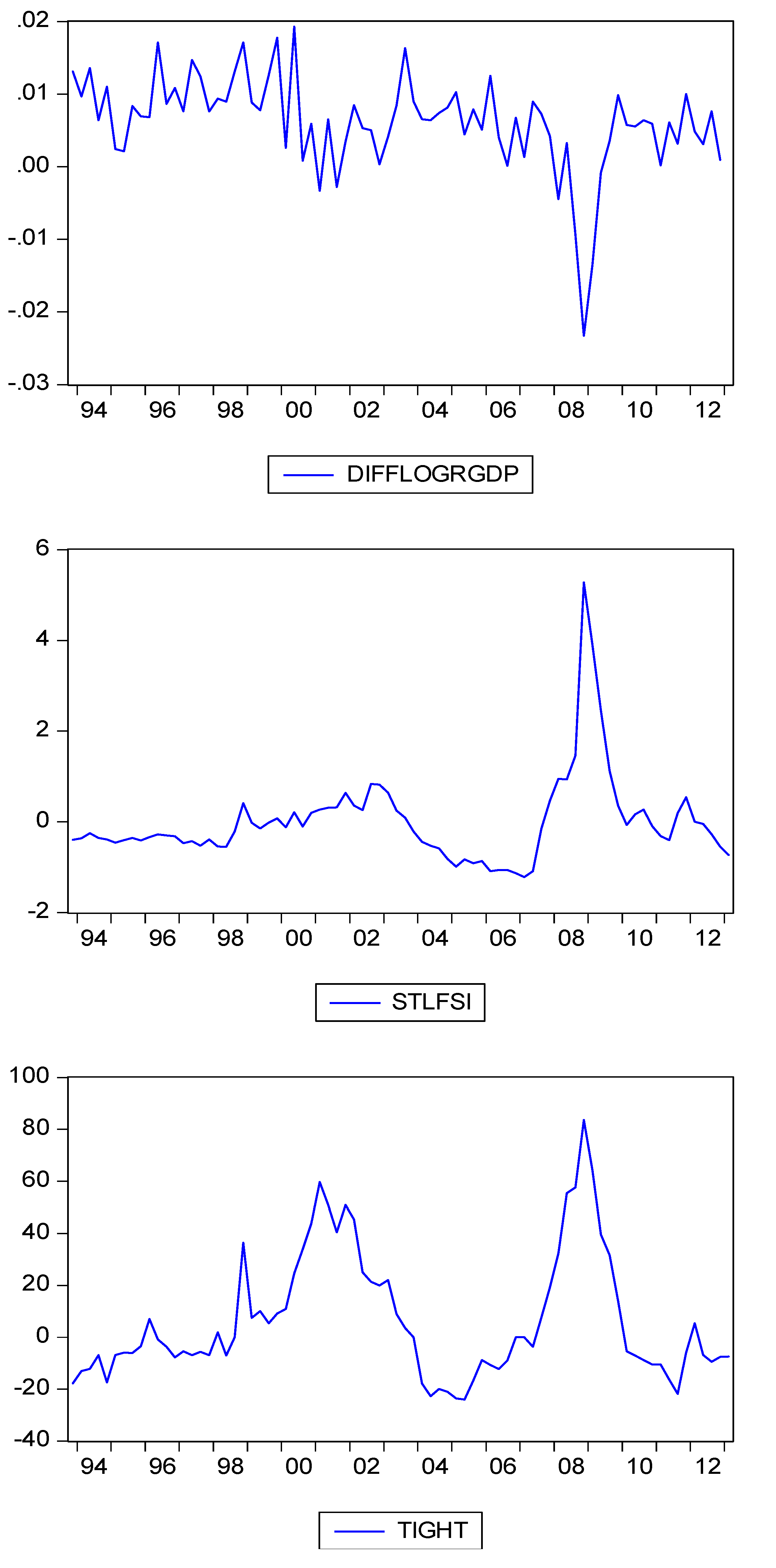
Inspection of the graphs in Figure 1 shows the three variables to be stationary, though quite persistent, particularly during the crisis period, so care is need for the proper specification. The sample 1993Q4-2013Q1 reflects the entire history of the variable STLFSI. Results for the Augmented Dickey-Fuller test on levels of the data are reported in Table 1, and shows that one can reject a unit root in all three variables at a significance level of 5% or better. The number of lags is determined by the Akaike Information Criterion.
Figure 1.
Time series graphs of the endogenous variables over the sample 1993Q4-2013Q1. DIFFLOGRGDP is the log difference of real GDP for the U.S. STLFSI is the St. Louis Fed stress indicator, and TIGHT is the percentage of loans officer reporting a tightening of standards.
Figure 1.
Time series graphs of the endogenous variables over the sample 1993Q4-2013Q1. DIFFLOGRGDP is the log difference of real GDP for the U.S. STLFSI is the St. Louis Fed stress indicator, and TIGHT is the percentage of loans officer reporting a tightening of standards.

Table 1.
Each row contains results of the Augmented Dickey-Fuller test. The number of lags was chosen according to the Akaike criterion.
| lags | t - statistic | prob | |
|---|---|---|---|
| DIFFLOGRGDP | 1 | −3.38 | 0.01 |
| STLFSI | 1 | −3.14 | 0.03 |
| TIGHT | 3 | −3.20 | 0.02 |
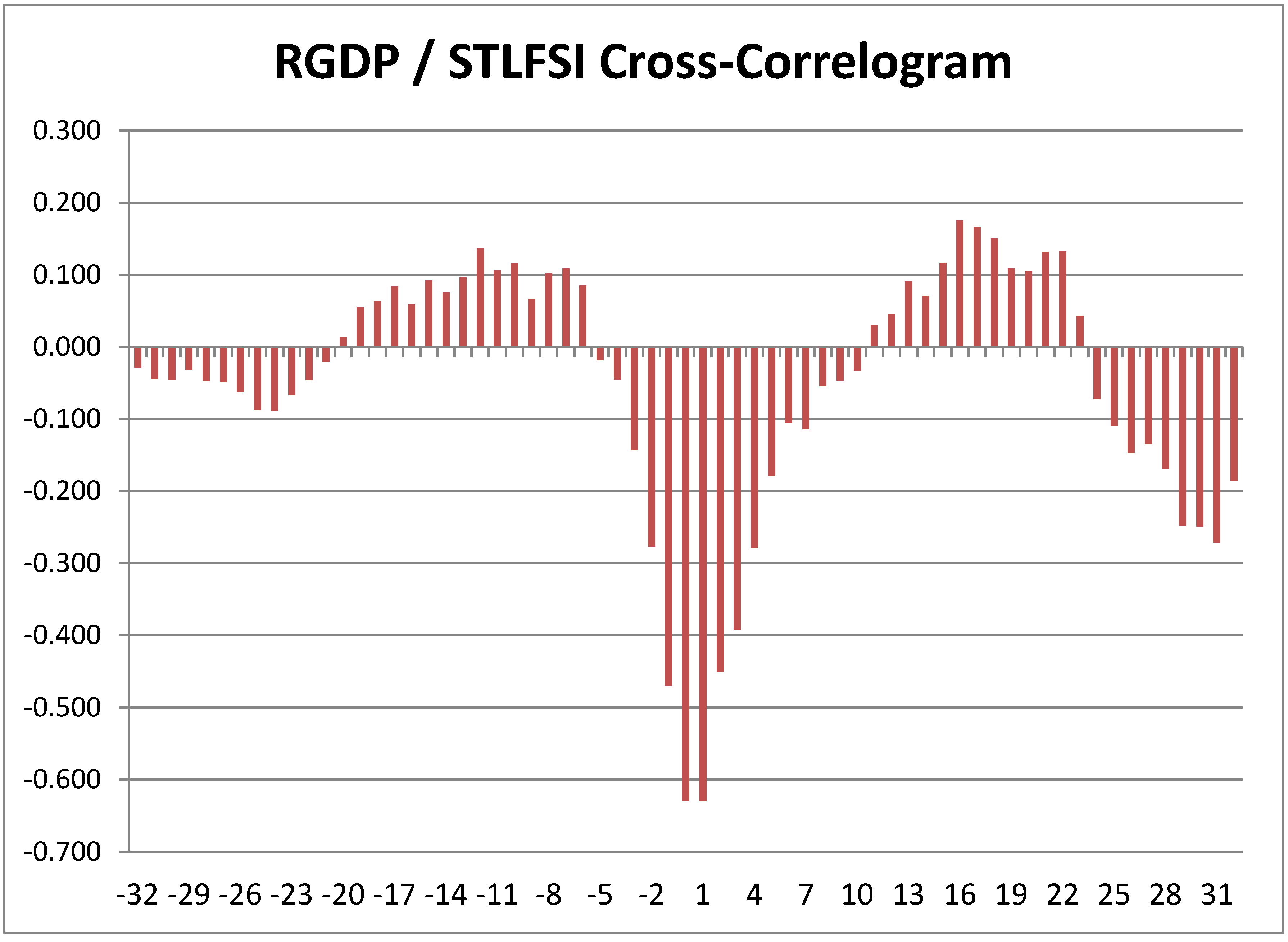
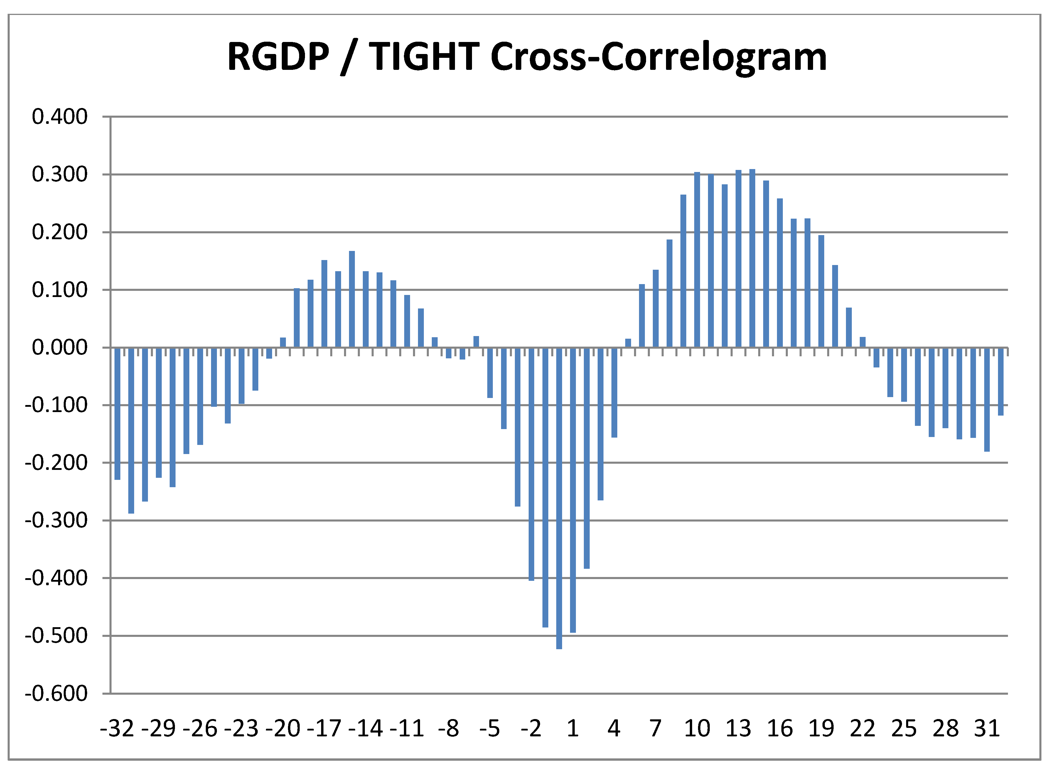
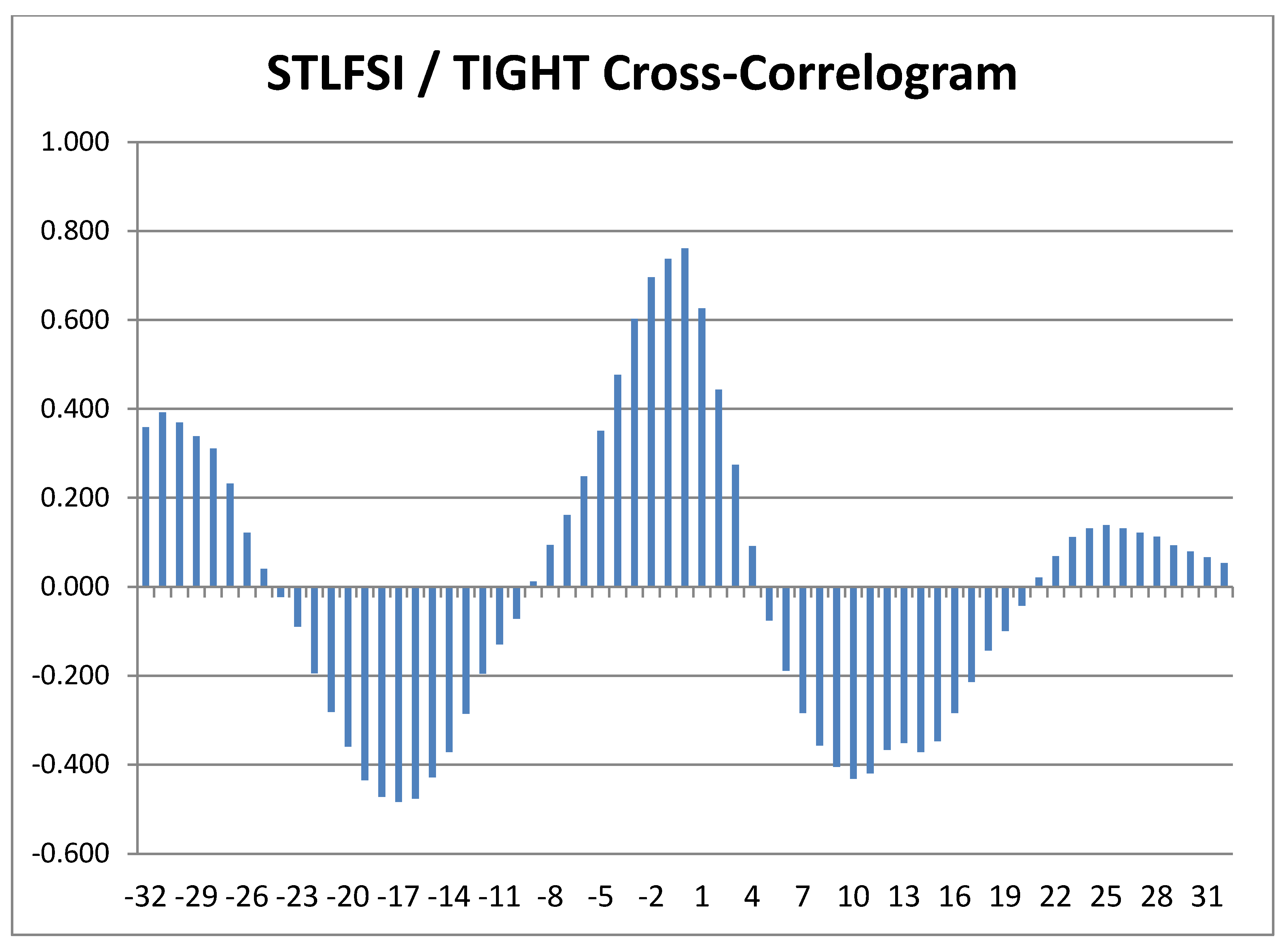
Preliminary examination of the cross-correlograms in Figure 2, Figure 3, Figure 4 show anticipated relationships between the three variables. There is a negative contemporaneous relationship between log differenced real GDP and the two measures of credit market conditions and a positive contemporaneous relationship between STLFSI and TIGHT. However, the cross-correlograms also show a great deal of persistence, so any conclusions about causality require formal testing.
Figure 2.
Cross-Correlogram with lags and leads on the x-axis. See Figure 1 caption for sample details.
Figure 2.
Cross-Correlogram with lags and leads on the x-axis. See Figure 1 caption for sample details.

Figure 3.
Cross-Correlogram with lags and leads on the x-axis. See Figure 1 caption for sample details.
Figure 3.
Cross-Correlogram with lags and leads on the x-axis. See Figure 1 caption for sample details.

Figure 4.
Cross-Correlogram with lags and leads on the x-axis. See Figure 1 caption for sample details.
Figure 4.
Cross-Correlogram with lags and leads on the x-axis. See Figure 1 caption for sample details.
Estimation of the unrestricted VAR shows considerable auto-correlation in the residuals requiring the inclusion of at least seven lags3. Since all variables are integrated of the same order, the Wald test for Granger causality has the standard χ² distribution. Results for this test are reported in Table 2.
Table 2.
Each statistic (not in parentheses) is the test for whether to column variable Granger causes the dependent variable in the row. The numbers in parentheses are p-values for the null of no causality.
| DIFFLOGRGDP | STLFSI | TIGHT | |
|---|---|---|---|
| DIFFLOGRGDP | 4.67 | 22.36 | |
| (0.700) | (0.002) | ||
| STLFSI | 12.83 | 15.09 | |
| (0.076) | (0.035) | ||
| TIGHT | 5.08 | 4.40 | |
| (0.650) | (0.733) |
As noted above, TIGHT Granger causes DIFFLOGRGDP at a high level of significance, but STLFSI does not at any reasonable level of significance. Lending standards and quantity rationing of credit are much more important than lending costs for explaining fluctuations in real activity. The lending standards variable and the log difference of real GDP both Granger cause STLFSI. The credit market stress indicator is correlated to the other variables, but the lending standards variable has much more explanatory power. Change in the ordering of the variables does not make any qualitative difference in the results.
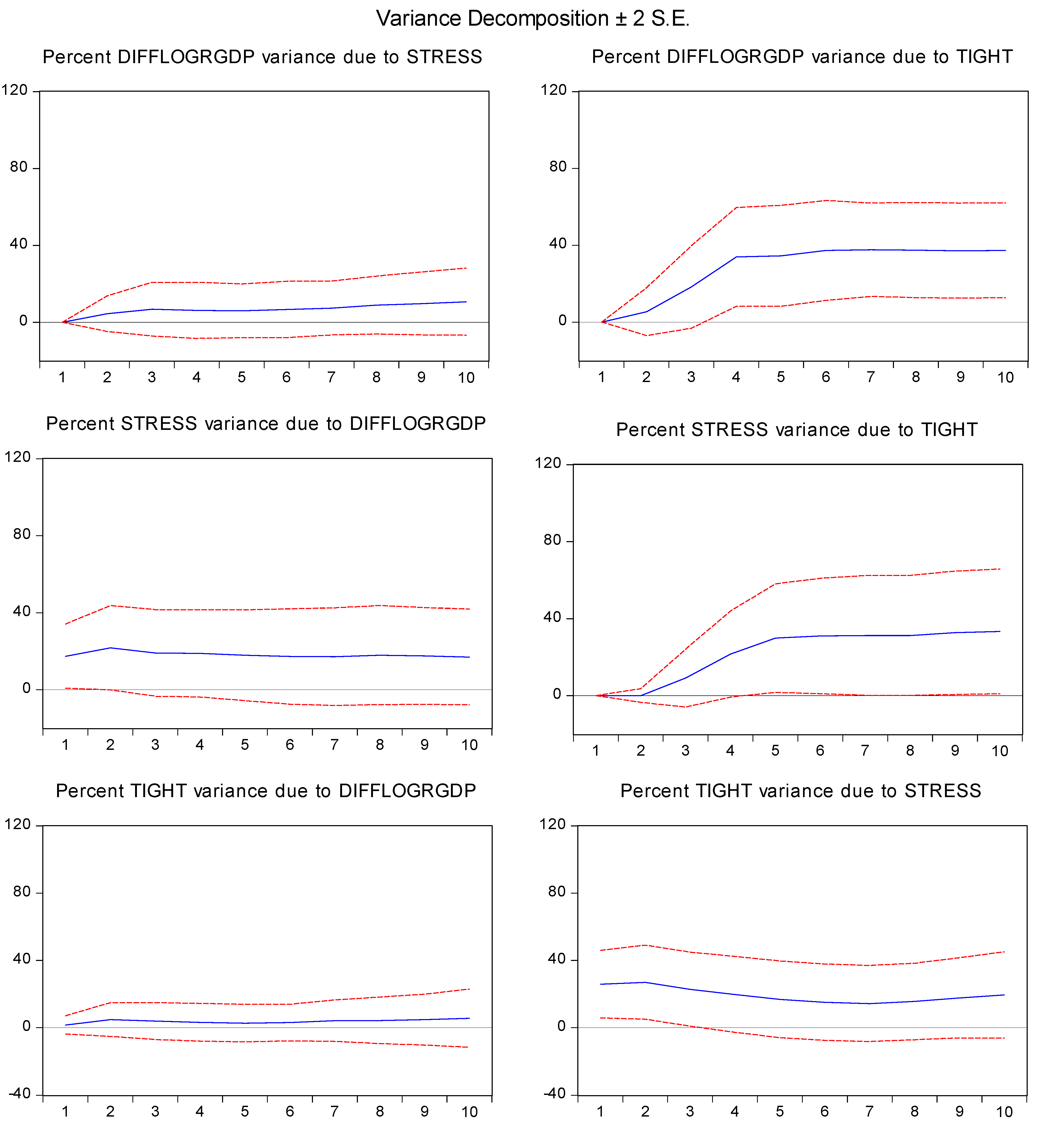
Graphs of the impulse response functions and variance decomposition in Figure 5, Figure 6 show that there is an intuitive relationship between the three variables. Real GDP declines with an increase in the financial markets stress indicator and a tightening of lending standards. STLFSI and TIGHT are positively correlated as expected. The variance decomposition graphs confirm that the loan officer survey data on standards has greater explanatory power for both real GDP and the stress indicator.
Figure 5.
Impulse response functions for the three variable VAR with seven lags. The red lines are 5% confidence intervals.
Figure 5.
Impulse response functions for the three variable VAR with seven lags. The red lines are 5% confidence intervals.

Figure 6.
Variance decomposition results for the three variable VAR with seven lags. The red lines are 5% confidence intervals.
Figure 6.
Variance decomposition results for the three variable VAR with seven lags. The red lines are 5% confidence intervals.

Conclusions
The results show evidence that quantity rationing of credit is a key determinant in the relationship between financial markets and the real economy. Price rationing, as measured by interest rates, remains closely correlated with macro variables, but the present work shows that lending standards as represented by the loan officer survey data has greater importance as a leading indicator.
- 1. See Lown and Morgan [2] for a detailed description of the lending standards data.
- 2. The St. Louis Fed’s Financial Stress Index is a composite of seven interest rates, six interest rate spreads, two volatility indices, a bond fund, and financial equities index and the spread between the 10-year U.S. Treasury and TIPS bonds. See [6] for complete details.
- 3. The choice of seven lags is made according to the sequential modified likelihood ratio test. Furthermore, the Portmanteau test statistic is 16.67, meaning the null hypothesis of no autocorrelation in the residuals cannot be rejected at the 5% level for up to 7 lags.
Conflict of Interest
The author declares no conflict of interest.
References
- G. Waters. “Quantity Rationing of Credit.” Bank of Finland Discussion Paper, 2012. No. 3/2012. [Google Scholar]
- C. Lown, and D. Morgan. “The Credit Cycle and the Business Cycle: New Findings Using the Loan Officer Opinion Survey.” J. Money Credit Bank. 38 (2006): 1574–1597. [Google Scholar]
- A. Estrella, and F. Mishkin. “The Predictive Power of the Term Structure of Interest Rates in Europe and the United States: Implications for the European Central Bank.” Eur. Econ. Rev. 41 (1997): 1375–1401. [Google Scholar] [CrossRef]
- K. Kliesen, M. Owyang, and E.K. Vermann. “Disentangling Diverse Measures: A Survey of Financial Stress Indexes.” Fed. Reserv. Bank St. Louis Rev. 94 (2012): 369–397. [Google Scholar]
- S. Aramonte, S. Rosen, and J.W. Schindler. “Assessing and Combining Financial Conditions Indexes.” Finance and Econonics Discussion Series of the Board of Governors of the Federal Reserve. 30 May 2013. No. 2013-39. Available online: http://www.federalreserve.gov/pubs/feds/2013/201339/201339pap.pdf (accessed on 19 June 2013).
- Federal Reserve Bank of St. Louis. “Appendix.” National Economic Trends. January 2010. Available online: http://research.stlouisfed.org/publications/net/NETJan2010Appendix.pdf (accessed on 19 June 2013).
© 2013 by the authors; licensee MDPI, Basel, Switzerland. This article is an open access article distributed under the terms and conditions of the Creative Commons Attribution license (http://creativecommons.org/licenses/by/3.0/).
Share and Cite
MDPI and ACS Style
Waters, G.A. Quantity versus Price Rationing of Credit: An Empirical Test. Int. J. Financial Stud. 2013, 1, 45-53. https://doi.org/10.3390/ijfs1030045
AMA Style
Waters GA. Quantity versus Price Rationing of Credit: An Empirical Test. International Journal of Financial Studies. 2013; 1(3):45-53. https://doi.org/10.3390/ijfs1030045
Chicago/Turabian StyleWaters, George A. 2013. "Quantity versus Price Rationing of Credit: An Empirical Test" International Journal of Financial Studies 1, no. 3: 45-53. https://doi.org/10.3390/ijfs1030045