Machine Learning to Forecast Financial Bubbles in Stock Markets: Evidence from Vietnam

Department of Banking, Ho Chi Minh University of Banking, No. 36 Ton That Dam Street, Nguyen Thai Binh Ward, District 1, Ho Chi Minh City 700000, Vietnam
*
Author to whom correspondence should be addressed.
Int. J. Financial Stud. 2023, 11(4), 133; https://doi.org/10.3390/ijfs11040133
Submission received: 26 September 2023
/
Revised: 3 November 2023
/
Accepted: 6 November 2023
/
Published: 8 November 2023
Abstract
:Financial bubble prediction has been a significant area of interest in empirical finance, garnering substantial attention in the literature. This study aims to detect and forecast financial bubbles in the Vietnamese stock market from 2001 to 2021. The PSY procedure, which involves a right-tailed unit root test to identify the existence of financial bubbles, was employed to achieve this goal. Machine learning algorithms were then utilized to predict real-time financial bubble events. The results revealed the presence of financial bubbles in the Vietnamese stock market during 2006–2007 and 2017–2018. Additionally, the empirical evidence supported the superior performance of the random forest and artificial neural network algorithms over traditional statistical methods in predicting financial bubbles in the Vietnamese stock market.
1. Introduction
Financial bubbles can have profound effects on an economy and the livelihoods of its citizens. Consequences, such as financial and debt crises, as seen in the dot-com bubble of 1999–2001 and the U.S. subprime mortgage crisis of 2007–2009, often originate from the abnormal escalation of asset prices in the stock market or the real estate market. When a bubble bursts, it can lead to the collapse of major financial institutions, pushing countries to the brink of bankruptcy and triggering comprehensive financial and economic crises. Governments are forced to allocate substantial resources to bailout packages and recovery programs in the wake of such crises.
Moreover, the social costs remain significant, and the restoration of public confidence in the market poses a particularly formidable challenge. Inexperienced investors, lacking the knowledge to manage risks, are among the most severely impacted (Galbraith et al. 2009). They often hold assets during the late stages of a bubble, making them particularly vulnerable to the adverse effects of the bubble’s burst. Therefore, for governments and market supervisors, researching and forecasting the status of financial bubbles is extremely important. This enables the implementation of necessary interventions to mitigate adverse impacts of financial bubbles on the market and society, especially in the context of globalization where risks can easily spread between markets.
The Vietnamese stock market was established in July 2000 with the launch of the Ho Chi Minh City Stock Exchange. The market experienced significant growth from 2006 to 2007, thanks to foreign investment inflows following Vietnam’s entry into the WTO and the enactment of the Securities Law in 2006. However, there was a sharp decline in 2008, followed by a recovery in 2009, leading to stable growth until 2016. From 2017 to the present, the Vietnamese stock market has been characterized by significant volatility, with the VNIndex surpassing the 1000-point mark in 2018, followed by a sharp decline in 2020, and continued fluctuations from 2021 to 2022. Vietnam Stock Market Capitalization accounted for USD 205.153 billion in July 2023, which is equivalent to 65% of the GDP. There are over 1600 listed companies in the market, with the majority operating in the financial, real estate, and essential consumer goods sectors, accounting for over 80% of the total market capitalization. Although the Vietnamese market is developing quickly, it still lacks efficiency and sustainability. The market is typically sensitive to rumours and contains many stocks that are manipulated in price. These issues may arise from a lack of transparency in market information and volatility in investor sentiment. Therefore, regulatory authorities must be vigilant in detecting financial bubbles early to safeguard retail investors and maintain market stability.
Machine learning has been increasingly gaining attention from researchers as it offers a promising solution to address a wide range of forecasting issues, such as predicting financial crises (Alessi and Detken 2018; Beutel et al. 2019; Chatzis et al. 2018; Ouyang and Lai 2021), default predictions (Barboza et al. 2017; Fuster et al. 2022; Geng et al. 2015; Shin et al. 2005; Tran et al. 2022; Zhao et al. 2015), or forecasting stock price trends (Cakici et al. 2023; Dong et al. 2022; Gu et al. 2020; Zhou et al. 2023). Based on the literature, machine learning algorithms have demonstrated better outcomes than traditional statistical models in both classification and time-series regression problems. However, it is important to note that forecasting results can vary significantly across models depending on the dataset used, and there is no one-size-fits-all approach that can guarantee a superior performance.
In the field of macroeconomics, the use of machine learning for identifying financial bubbles in the stock market is a relatively new approach and has received limited research attention. Most studies on financial crises in banking, securities markets, and public debt have focused on predicting general economic crises, rather than forecasting individual financial bubbles. To date, only one recent study conducted by Başoğlu Kabran and Ünlü (2021) has explored the use of machine learning techniques for predicting financial bubbles. There is also a lack of research on financial bubbles in Vietnam, especially when it comes to quantitative methodologies and machine learning algorithms. The academic community still debates and remains skeptical about the effectiveness of forecasting tools that use machine learning algorithms.
The main objective of our research is to detect financial bubbles in the Vietnamese stock market from 2001 to 2021 and subsequently forecast financial bubble occurrences based on macroeconomic indicators. We employed the PSY procedure to identify market phases with bubble-like characteristics and use machine learning algorithms for prediction. Furthermore, we implemented the SMOTE method to rectify data imbalances within the dataset and leveraged the PCA method to reduce data dimensionality, thereby enhancing the quality of our forecasting outcomes. We aim to determine the best-performing model among the methods used. We anticipate that our study can contribute empirical evidence regarding the application of machine learning for the real-time forecasting of financial bubbles. This can provide early warning signals for policymakers and investors to make informed financial decisions.
The remaining sections of this research paper are organized as follows: Section 2 introduces the theoretical framework for detecting financial bubbles and the application of machine learning in forecasting. Section 3 outlines our data sources and methodologies, including the PSY procedure and machine learning techniques. Section 4 presents our research findings and thoroughly discusses their implications. Finally, Section 5 provides a concise conclusion, summarizing key insights and suggesting avenues for future research.
2. Literature Review
2.1. Definition of Financial Bubbles
In theory, the concept of financial bubbles is often referred to by various terms, like asset price bubbles or speculative bubbles, and is an intriguing research topic. There are various perspectives on financial bubbles and their identification. However, attempting to classify and provide a clear-cut definition remains a controversial subject within the academic community. Generally, the classification of financial bubbles falls into two primary categories: classical bubbles and modern bubbles.
Classical bubbles are primarily driven by irrational investor behavior. Shiller (2002) posits that bubbles in the market are a psychological phenomenon. He suggests that the occurrence of these bubbles is a result of amplified feedback-trading tendencies, which are caused by the attention paid to them by news media. The reason for this is that, as more investors show interest in a particular asset, news media tend to expand their coverage of it, which in turn attracts even more potential investors. This leads to an increase in demand for the asset, which causes its price to rise, thereby attracting even more attention from the news media. This cyclical process reinforces the feedback-trading tendency in the market, ultimately leading to the occurrence of bubbles. This phenomenon is often referred to as ‘herd mentality’, and its consequences can lead to a severe market collapse, subsequently exerting a profound impact on the overall economy. Kindleberger et al. (2005) proposed an approach to understanding financial bubbles from the perspectives of irrational exuberance and psychological expectations. According to these authors, financial bubbles were created by the irrational exuberance and blind faith of investors, leading to a series of reckless investment decisions and ultimately culminating in a market collapse and asset value correction. Stiglitz (1990) suggested that the phenomenon of a financial bubble occurs when investors believe that current prices already reflect high levels of expectations, and the fundamental factors supporting those prices are no longer in place. In other words, when investors believe that current prices no longer offer them the potential for future profits and this sentiment becomes widespread, a bubble begins to form. When investors have faith that the upward trend will continue and fear missing out on potential gains if they do not buy at the present moment, the bubble inflates. However, a bubble will be prone to burst when investors start to believe that prices can no longer rise further, demand wanes, and this can trigger a significant sell-off, causing prices to fall rapidly (Case and Shiller 2003).
The second approach is the modern bubble, described by Tirole (2008) as a situation in which the price of an asset exceeds its fundamental value. The fundamental value of an asset is typically based on its expected future cash flows, such as dividends, coupon payments, or rental income. According to the author, bubbles occur when investors are willing to pay a higher price for an asset that can be resold immediately than if they were obligated to hold onto it for a longer period. This view recognizes that an asset’s perceived value is not always tied to its true value, but rather to its potential for short-term profits. In the derivatives market, a bubble is considered to exist if the market value of a derivative consistently exceeds the cost of creating similar derivatives. This means that the price at which the derivative is trading in the market is higher than the cost of creating a comparable derivative. An illustration of such a bubble can be observed in the price disparity in option pricing. Specifically, a bubble may occur when a combination of put and call options, designed to replicate the movements of a stock, is traded at a price differential compared to the price of the underlying stock. This price differential must also take into account factors such as interest rates and the cost of borrowing the stock. Therefore, the existence of bubbles in various forms highlights the complexity of market dynamics and raises the challenges associated with maintaining economic stability.
Additionally, the concept of bubbles can be classified into two categories: rational bubbles and partially rational bubbles. The rational bubble theory proposes that investors knowingly purchase overpriced assets with the understanding that they can sell them at a profit in the future. This theory posits that, even when faced with prices that are clearly overvalued, expectations of future profits can drive investment behavior. In other words, investors in rational bubbles willingly engage in the bubble, motivated by the prospect of profiting from price increases before the bubble eventually bursts. Shiller (2015) introduced the concept of partially rational bubbles, which posits that stock prices are influenced by a combination of rational and irrational behavior among investors. He suggested that individual investors were prone to irrational exuberance, often driven by sensationalized media reports, but this does not mean that investors are consistently irrational or ‘crazy’. Rather, the stock market is influenced by social trends and short-term desires, which may either lead to the formation of bubbles or not. In essence, partially rational bubbles recognize that market behavior can be influenced by both rational and irrational elements that stem from societal trends and collective beliefs, and these factors contribute to the persistence of bubbles. This perspective provides a more nuanced understanding of the dynamics that drive financial bubbles.
Fama (2014), who advocates the Efficient Market Hypothesis (EMH), offers an alternative perspective on financial bubbles. According to Fama, the extreme price fluctuations of assets can be anticipated, and as a result, there are no bubbles in asset prices. While this stance is still subject to debate, it provides a framework for delving into the identification of factors or causes that could lead to the predictable formation of bubbles. Fama’s view challenges the perception that financial bubbles are irrational and uncontrollable, and proposes that there may be underlying patterns and elements that can be used to predict or understand the emergence of bubbles. This perspective has given rise to further research into the predictability of bubbles and the factors that contribute to their formation.
In this article, we approach bubbles from the perspective of irrational bubbles, which are characterized by a sudden surge in prices within a short time frame followed by a rapid decline in the VNINDEX. Additionally, we also recognize the presence of the external factors that influence market dynamics beyond investor behavior, as posited by Fama’s perspective.
2.2. Literature Review on Detecting Financial Bubbles
Throughout history, a multitude of research studies have been conducted with the objective of identifying bubbles in financial markets that are characterized by speculation, including but not limited to stock markets, foreign exchange markets, real estate markets, and, more recently, cryptocurrency markets. However, within the context of this article, we provide a concise overview of studies conducted solely within the sphere of the stock market, with a particular focus on those that utilize statistical models on time-series data.
Shiller (1981) introduced a novel method called Variance Bounds Tests, which he applied to sample data of the S&P price index from 1871 to 1979, revealing evidence of a bubble existence. However, Shiller’s approach is often deemed less reliable when applied to small sample sizes.
West (1987) employed Euler equations and ARIMA models on annual stock price and dividend data of the S&P 500 from 1871 to 1980 and the Dow Jones index from 1928 to 1978, providing robust statistical evidence of the existence of stock market bubbles in the United States.
Phillips et al. (2011) proposed the Sup Augmented Dickey–Fuller test (SADF), also known as the PWY method, to assess the presence of rational bubbles in financial markets. This approach is based on the null hypothesis of a unit root, analogous to the conventional Dickey–Fuller test, but with a right-tailed alternative hypothesis. Rejecting the null hypothesis in this test indicates the presence of explosive behavior in the price series, thereby providing empirical evidence for the existence of a bubble. The right-tailed SADF unit root tests are conducted using rolling window forms. Homm and Breitung (2012) applied this test to detect stock market bubbles, and after a process of simulation and evaluation criteria comparison, the authors found that the SADF test was the most optimal among the methods employed. The SADF test is effective when there is a single bubble event, but in practical applications, there may be multiple bubbles appearing in sufficiently large samples. While this method successfully identified famous historical bubbles, the SADF test failed to detect the 2007–2008 debt crisis bubble.
Phillips et al. (2015a) developed the Generalized sup ADF (GSADF) test as an improvement over the SADF method, also referred to as the PSY procedure, to overcome its limitations. The GSADF test is an iterative application of the right-tailed ADF test based on the rolling-window SADF test that aims to detect explosive patterns in sample sequences. Compared to the SADF, the GSADF is more flexible in terms of rolling windows, making it a valuable tool for investigating price explosion behavior and confirming the presence of market bubbles. In their study, they applied both the SADF and GSADF tests to the S&P 500 index from 1871 to 2010, revealing that the GSADF successfully identified two bubble periods: the Panic of 1873 (from October 1879 to April 1880) and the dot-com bubble (from July 1997 to August 2001). When restricting the bubble duration to over 12 months, the results showed that there were three existing bubble periods: the post-1954 war period, Black Monday in 1987, and the dot-com bubble in 2000.
Based on the findings outlined above, it is evident that the GSADF test is an effective approach for detecting the presence of market bubbles. Hence, in this study, we employ the PSY procedure to identify the existence of bubbles in the Vietnamese stock market.
2.3. Literature Review on Machine Learning Applied to Economic Forecasting
In macroeconomics, machine learning techniques are commonly used for classification problems, such as predicting stock market trends and corporate bankruptcies. While the use of machine learning for identifying financial bubbles in the stock market is a relatively new approach and has been the subject of limited research, most studies on financial crises in banking, securities markets, and public debt have focused on predicting general economic crises rather than forecasting individual financial bubbles. To date, only one recent study by Başoğlu Kabran and Ünlü (2021) has been conducted on predicting financial bubbles. The authors used a support vector machine (SVM) approach to forecast bubbles in the S&P 500 index and compared it to other methods. The results demonstrated that SVM has a superior performance in predicting financial bubbles.
Several notable studies have been conducted to forecast financial crises. Alessi and Detken (2018) constructed a warning system using random forest to identify systemic risk from a dataset of banking crises in the EU, using macroeconomic indicators as predictors. Their results demonstrated that the random forest model provided an excellent predictive performance and holds promise for macroeconomic forecasting. Beutel et al. (2019) compared the out-of-sample predictive performance of various early warning models for systemic banking crises in advanced economies and found that while machine learning methods often exhibit high in-sample fits, they were outperformed by the logit approach in recursive out-of-sample evaluations. Chatzis et al. (2018) utilized a wide range of machine-learning algorithms to forecast economic risks across 39 countries. They demonstrated that deep neural networks significantly improved classification accuracy and provided a robust method to create a global systemic early warning tool that is more efficient and risk-sensitive compared to the established methods. Ouyang and Lai (2021) proposed an Attention-LSTM neural network model to assess systemic risk early warning in China. They found that the model exhibited superior accuracy compared to other models, suggesting that it could be a valuable tool for systemic risk assessment and early warning in the Chinese context.
In default prediction, machine learning models have also demonstrated superiority in handling non-linear relationships compared to traditional models. Shin et al. (2005) employed SVM to forecast bankruptcy for 2320 medium-sized enterprises in the Korean Credit Guarantee Fund from 1996 to 1999. The study’s outcomes showed that SVM provided superior predictive outcomes compared to other models, including artificial neural network (ANN) models. Zhao et al. (2015) conducted research to develop a credit scoring system based on ANN employing a credit dataset from Germany. The study’s results demonstrated that ANN could forecast credit scores more accurately than traditional models, obtaining an accuracy rate of 87%. Geng et al. (2015) utilized machine learning models to predict financial distress for companies listed on the Shanghai and Shenzhen stock exchanges from 2001 to 2008. The study’s findings revealed that the ANN model yielded better results when compared to decision trees, SVM, and random forest models. Barboza et al. (2017) applied SVM, ensembles, boosting, and random forest methods to predict bankruptcy for 10,000 companies in the North American market from 1985 to 2013. The authors contrasted these models with traditional statistical models and examined their predictive performance. The results indicated that ensemble methods, like bagging, boosting, and random forests, outperformed other approaches. Specifically, machine learning models achieved an average accuracy that was approximately 10% higher than traditional models. The random forest model displayed the highest accuracy, reaching up to 87%, whereas traditional models ranged from 50% to 69% accuracy. Fuster et al. (2022) examined mortgage default cases in the United States and found that the random forest model achieved a higher predictive accuracy than logistic regression. These results highlight the effectiveness of ensemble methods, particularly random forests, in financial distress prediction compared to traditional models. A recent study conducted by Tran et al. (2022) incorporated the Shapley values to clarify the forecasting outcomes of complex machine learning models on a dataset of listed companies in Vietnam from 2010 to 2021. The study’s results showed that the extreme gradient boosting and random forest models outperformed other models. One interesting point is that, based on Shapley values, the authors determined the influence of each feature on the prediction results and provided additional insights into relationships that are not present in theory.
Interesting findings have emerged from studies exploring how machine learning can be applied to the prediction of stock price trends. Gu et al. (2020) explored the use of machine learning techniques for empirical asset pricing. Their study revealed that investors can benefit significantly from using machine learning predictions. In fact, in some cases, these predictions can lead to twice the performance when compared to well-established regression-based strategies found in the existing literature. The authors identified decision trees and neural networks as the top-performing methods, attributing their superior predictive capabilities to their ability to capture intricate non-linear interactions among predictors that are often overlooked by other approaches. Additionally, the study revealed a consensus among all methods regarding a relatively limited set of dominant predictive indicators. The most influential predictors were linked to price-related factors, such as return reversal and momentum, while measures of stock liquidity, stock volatility, and valuation ratios emerged as the next most potent predictors in the context of asset pricing. The study conducted by Cakici et al. (2023) delved into the issue of equity anomalies predicting market risk premiums. The study analyzed updated data from both the U.S. and global markets, utilizing various machine learning techniques. The study covered 42 countries from January 1990 to December 2021. The researchers concluded that anomalies, in their typical form, cannot forecast overall market returns. However, this conclusion is only applicable to the U.S. and lacks external validity in two aspects. Firstly, it cannot be generalized to international contexts. Secondly, it is not accurate for different sets of anomalies, irrespective of how factor strategies are selected and designed. The study found that, if there is any predictability, it is limited to a small number of specific anomalies and is heavily influenced by seemingly minor methodological decisions. Dong et al. (2022) aimed to explore the connection between long–short anomaly portfolio returns and the predictability of the aggregate market excess return over time. The researchers analyzed 100 representative anomalies from the literature and incorporated various shrinkage techniques, such as machine learning, forecast combination, and dimension reduction, to provide the first systematic evidence on this correlation. The study concluded that long–short anomaly portfolio returns have significant out-of-sample predictive ability for the market excess return, both statistically and economically. The authors attributed this predictive ability to the asymmetric limits of arbitrage and overpricing correction persistence. The study emphasized the importance of using representative groups of long–short anomaly portfolio returns from the cross-sectional literature to predict the market excess return on an out-of-sample basis, provided that forecasting strategies that guard against overfitting the data are used. Zhou et al. (2023) conducted a recent study where they utilized deep neural network (DNN) models to make predictions on equity premiums. The study analyzed a dataset that covered monthly data from December 1950 to December 2016 and computed equity premiums as the difference between the log return on the S&P 500 (including dividends) and the log return on a risk-free bill. The aim of the study was to evaluate and compare the predictive ability of DNN models with that of ordinary least squares (OLS) models and historical average (HA) models. The researchers found that DNN models were the most effective and significantly outperformed both OLS and HA models in both in-and out-of-sample tests as well as asset allocation exercises. The DNN model’s forecasting performance was further improved by the inclusion of 14 additional variables that were selected from the finance literature. This indicates that the DNN model comprehensively incorporates the predictive information contained in these variables. The researchers suggest that the DNN’s superior performance may be attributed to its ability to automatically extract high dimensional features from data and discover different forecasting patterns in the data.
The literature suggests that machine learning algorithms exhibit better outcomes than statistical models in both classification and time-series regression problems. Nevertheless, the forecasting results across models can differ considerably depending on the dataset used, and there is no one-size-fits-all superior approach. Several factors can significantly impact forecasting results, such as data imbalance, the presence of outliers in the dataset, and the selection of parameters within the models. In this case, the choice of the forecasting model is of utmost importance and can significantly impact the output results. Therefore, the primary aim of this research is to identify and select the most appropriate model for forecasting financial bubbles in the Vietnamese stock market. To our best knowledge, no prior research has been conducted on this topic.
3. Data
To identify financial bubbles in the stock market, we employed the Phillips, Shi, and Yu method (PSY method) on the Vietnam Stock Index (VN-Index) series collected from December 2001 to December 2021. The Vietnam Stock Index or VN-Index is a capitalization-weighted index of all the companies listed on the Ho Chi Minh City Stock Exchange. The dataset comprised a total of 252 data points, with 33 months identified as having financial bubbles. The method used for bubble identification was the PSY method, which is described in more detail in Section 4.2.
To facilitate the training and testing of our model, the data were partitioned into two main sets—the training set and the test set. The time chosen to split the dataset was January 2018, ensuring that the proportion of months with bubble phenomena in the training and test sets was 2/3 and 1/3, respectively. The objective here is to ensure that the training and testing datasets contain sufficient data for model development and evaluation.
In financial datasets, class imbalance is a commonplace phenomenon where the occurrence of financial bubbles is relatively infrequent compared to non-bubble periods. Our dataset also exhibited class imbalance, and to mitigate this issue, we employed the Synthetic Minority Over-sampling Technique (SMOTE). This approach was chosen due to its suitability for financial datasets where rare class occurrences are prevalent. SMOTE generates synthetic samples for the minority class, addressing the imbalance while preserving the data distribution characteristics. In financial markets, the accurate detection of financial bubbles is of utmost importance, and SMOTE assists in reducing bias, improving model generalization, and enhancing performance metrics, such as precision and recall. This technique ensures that the model can reliably identify critical financial bubble events with greater accuracy.
Given 55 macroeconomic indicator features in our dataset, we recognized the need to adopt a judicious strategy to mitigate the risk of overfitting. In this regard, we employed Principal Component Analysis (PCA) as a systematic means to condense the dimensions of our dataset. By transforming the original features into a smaller set of principal components, we retained the critical information essence while addressing the perils associated with excessive dimensions. This approach not only provides a practical solution to tackle the dimensionality conundrum but also serves as a catalyst for enhancing the efficacy of our machine learning model training, thereby augmenting prediction accuracy. It is important to note that, during the PCA process, feature scaling is applied through standardization using the StandardScaler tool from scikit-learn.
We chose the optimal number of principal components based on the cumulative-explained variance ratio. Specifically, we chose a threshold of 95% explained variance and selected the number of components that crossed that threshold. Based on Figure 1, the optimal number of components to retain is 7 components.
The identification of financial bubbles in the VNINDEX series was carried out by using the ‘psymonitor’ package in R to execute the PSY procedure as proposed by Phillips et al. (1984). Furthermore, for data analysis, Python and several associated packages, such as Numpy, Pandas, Scikit-learn, and Seaborn (Harris et al. 2020; McKinney 2010; Pedregosa et al. 2011; Waskom et al. 2017, respectively), were utilized.
4. Methodology
4.1. Research Design and Data Preprocessing
Our study was divided into two primary phases. Phase 1 involved the detection of financial bubbles in the stock market, while Phase 2 employed machine learning algorithms to predict the appearance of financial bubbles. The details of each phase are as follows:
In Phase 1, we focused on identifying financial bubbles in the Vietnamese stock market, utilizing historical stock market data, specifically the VNINDEX, from 2001 to 2021. This timeframe encompasses significant economic events and global economic fluctuations, particularly during the 2006–2008 and 2017–2018 periods, as noted by economic experts. Our goal was to identify financial bubble phenomena on a monthly basis during this time frame. We obtained daily stock index data from FiinPro, a reputable financial data provider in Vietnam.
In Phase 2, we used various machine learning techniques to predict the presence of financial bubbles. We utilized the macroeconomic indicators of Vietnam during the same timeframe to forecast financial bubble occurrences. The target variable was the financial bubble status for each month, as detected in Phase 1. We labeled months as 1 if a financial bubble occurred and 0 for other months. The forecasting time frame was one month prior. The features included macroeconomic variables collected from the World Bank data, representing crucial aspects of the economy, such as GDP growth, Consumer Price Index, broad money, foreign direct investment, and interest rate. In total, we selected 55 important macroeconomic indicators extracted from the World Bank dataset, considering them as features for forecasting. Most of the data are reported quarterly or annually; so, we employed the cubic spline interpolation method to convert them into monthly data while preserving the characteristic features of the variables.
4.2. PSY Method for Bubbles Detection
Within the scope of our research, we utilized the Phillips, Shi, and Yu (PSY) methodology, which employs recursive regression techniques to investigate the presence of a unit root in the face of an alternative right-tailed explosive hypothesis. This technique, which was introduced by Phillips et al. (2015b), was tailored to identify multiple bubble periods in a time series dataset. Rejecting the null hypothesis in this test was regarded as empirical evidence of the existence of financial asset price bubbles. The critical values for these tests were determined through Monte Carlo simulations, and the outcomes of these tests aid in defining the start and end dates of the bubbles.
The objective was to compute statistical measures on the right tail of the Augmented Dickey–Fuller (ADF) test with regard to a time series. Through a comparison of the maximum values that are derived from the test statistics with corresponding threshold values obtained from the distribution, analysts can draw inferences regarding the explosiveness of the observed values. The null hypothesis assumes that a time series follows a random walk process with an extremely small drift coefficient, as expressed by the following Equation:
where represents stock prices at time ; is the intercept; is the maximum lag; are the regression coefficients corresponding to different lags; and is the error term.
The recursive model is proposed as follows:
When conducting the test, the authors assumed a sample time frame of [0, 1]. The symbols and represent the estimated coefficients according to Equation (2) and the corresponding ADF test within the data window [], respectively. Let r_w denote the window size, so . The starting points r1 can vary within the range [0,].
The maximum ADF test statistic for the right tail is expressed by the following formula:
The PSY procedure assumes that the errors in the regression model, represented by , have a constant error variance. Based on this, the estimates of bubble periods using GSADF are determined by the following formulas:
where is the critical value of the SADF statistic based on observations .
with is the delayed SADF statistic related to the GSADF statistic by the following relationship:
In the PSY method, represents the minimum size, is the starting point, and is the ending point for each sample. The starting point is fixed, and varies from 0 to .
4.3. Machine Learning Methods to Predict Financial Bubbles
4.3.1. Logistic Regression
Logistic regression is a widely used statistical method for predictive modelling in scenarios where the response variable is binary. In the present study, the focus was on predicting financial distress. Based on the input features, the model generates a probability estimate of financial distress. This probability is computed through Equation (7).
Logistic regression is a commonly employed benchmark in research studies that investigate different forecasting methods. One of the key advantages of this technique is its ease of interpretation, which makes it accessible to most users. Therefore, logistic regression is frequently utilized in practical applications within financial institutions, owing to its high explanatory power.
4.3.2. Support Vector Machine
Support vector machines (SVMs) are a type of machine learning algorithm that relies on the concept of defining hyperplanes to partition observations in high-dimensional feature spaces. Linear SVM models prioritize the maximization of the margin between positive and negative hyperplanes. The classification decision is made using Equation (8).
where b is the bias.
In cases where the relationship between features and outcomes is non-linear, a kernel function is employed to transform the features into a higher dimensional space. A commonly used kernel function is the Gaussian radial basis function, which is expressed as Equation (9).
One of the strengths of support vector machines (SVMs) is their ability to avoid overfitting with small sample sizes and to remain robust to unbalanced distributions.
4.3.3. Decision Tree
Decision tree algorithms use a tree structure to extract insights from data and derive decision rules. The algorithm determines the optimal allocation for each split with maximum purity, using a measure such as the Gini coefficient or Entropy. The root node, representing the most distinguishing attribute, is located at the top of the tree, while the leaf nodes represent classes that correspond to the remaining attributes.
One of the main advantages of decision tree models is that they are intuitive and easy to interpret. However, there is a risk of overfitting during the feature domain division or branching process, which represents a potential drawback.
4.3.4. Random Forest
The random forest technique, which was developed by Breiman (2001), is based on the decision tree model. In random forests, decision trees are grown using a subset of randomly selected features. This random selection of both samples and features ensures the diversity of the basic classifiers. The forest is constructed from multiple subsets that generate an equal number of classification trees. The preferred class is identified based on a majority of votes, which results in more precise forecasts and, importantly, protects against overfitting the data.
4.3.5. Gradient Boosting (GB)
Gradient boosting is a machine learning technique commonly used in regression and classification tasks. It produces a prediction model in the form of an ensemble of weak prediction models, typically decision trees. Gradient boosting is a robust boosting algorithm that combines several weak learners into strong learners. In this technique, each new model is trained to minimize the loss function, such as mean-squared error or cross-entropy, of the previous model using gradient descent. During each iteration, the algorithm calculates the gradient of the loss function with respect to the predictions of the current ensemble and then trains a new weak model to minimize this gradient. The predictions of the new model are then added to the ensemble, and this process is repeated until a stopping criterion is met. This method has been proven to be effective in improving the prediction accuracy of models.
4.3.6. Artificial Neural Network
An artificial neural network, also known as a neural network, is a machine learning algorithm that is designed based on the structure and connections between neurons in the brain. This algorithm is capable of solving complex problems by mimicking the brain’s structure. An artificial neural network consists of many layers of artificial neurons, which are connected to one another. Each layer is composed of an input layer, output layer, and hidden layer. These artificial neurons simulate the role of real neurons through mathematical models. Each artificial neuron receives an input signal, , consisting of binary numbers (0 or 1). It then calculates the weighted sum of the signals it receives based on their weights, . The signal is only transmitted to the next artificial neuron when the sum of the weights of the received signals exceeds a certain threshold. An artificial neuron can be represented as Equation (10).
Based on historical data, neural network optimization is performed by determining the appropriate weights and activation thresholds. This process involves training the network using a set of input data and corresponding output data, which is used to adjust the weights and thresholds of the artificial neurons until the desired level of accuracy is reached. Through this iterative process, the neural network can learn to accurately predict outcomes for new input data.
4.4. Evaluation of the Model Performance
To evaluate the performance of classification algorithms, it is important to avoid focusing on a single class. Instead, a more comprehensive approach is preferred, which involves analyzing multiple metrics. The metrics are accuracy, precision, and sensitivity (recall).
Accuracy measures the proportion of correct classifications in the evaluation data and is calculated as follows:
Accuracy = (TP + TN)/(TP + TN + FP + FN)
Precision measures the proportion of true positives among the predicted positives and is calculated as follows:
Precision = TP/(TP + FP)
Sensitivity (recall) measures the proportion of positives that are correctly predicted and is calculated as follows:
Sensitivity (recall) = TP/(TP + FN)
In these equations, TP represents true positives, FP represents false positives, FN represents false negatives, and TN represents true negatives. By analyzing these metrics, the performance of different classification algorithms can be compared and evaluated.
In the case of imbalanced datasets, accuracy alone may not be a reliable metric for evaluating classification models. To provide a more comprehensive evaluation, the F1-score and the ROC curve are often used.
The F1 score is the harmonic mean of precision and sensitivity, ensuring that the F1-score is higher only when both components are higher. The F1 score is calculated as follows:
F1 Score = 2 × (Precision × Recall)/(Precision + Recall)
The ROC curve plots the true positive rate against the false positive rate, with the horizontal coordinate representing the false positive rate and the vertical coordinate representing the true positive rate. To quantify the characteristics of the ROC curve, the area under the curve (AUC) is introduced. The AUC value represents the area of the shadow part at the lower right of the ROC curve. The larger the shadow area, the greater the AUC value and the closer the ROC curve is to the upper left, indicating that the classification model is more accurate.
5. Results and Discussion
5.1. Results of the Financial Bubble Detection
In this study, we employed the PSY procedure to detect the presence of financial bubbles in the Vietnamese stock market from January 2001 to December 2021, on a monthly basis. The VNINDEX was determined on the last trading day of each month. The PSY procedure had a minimum window that includes at least 38 observations, as determined by the rule of . The monitoring process started from January 2001 onwards.
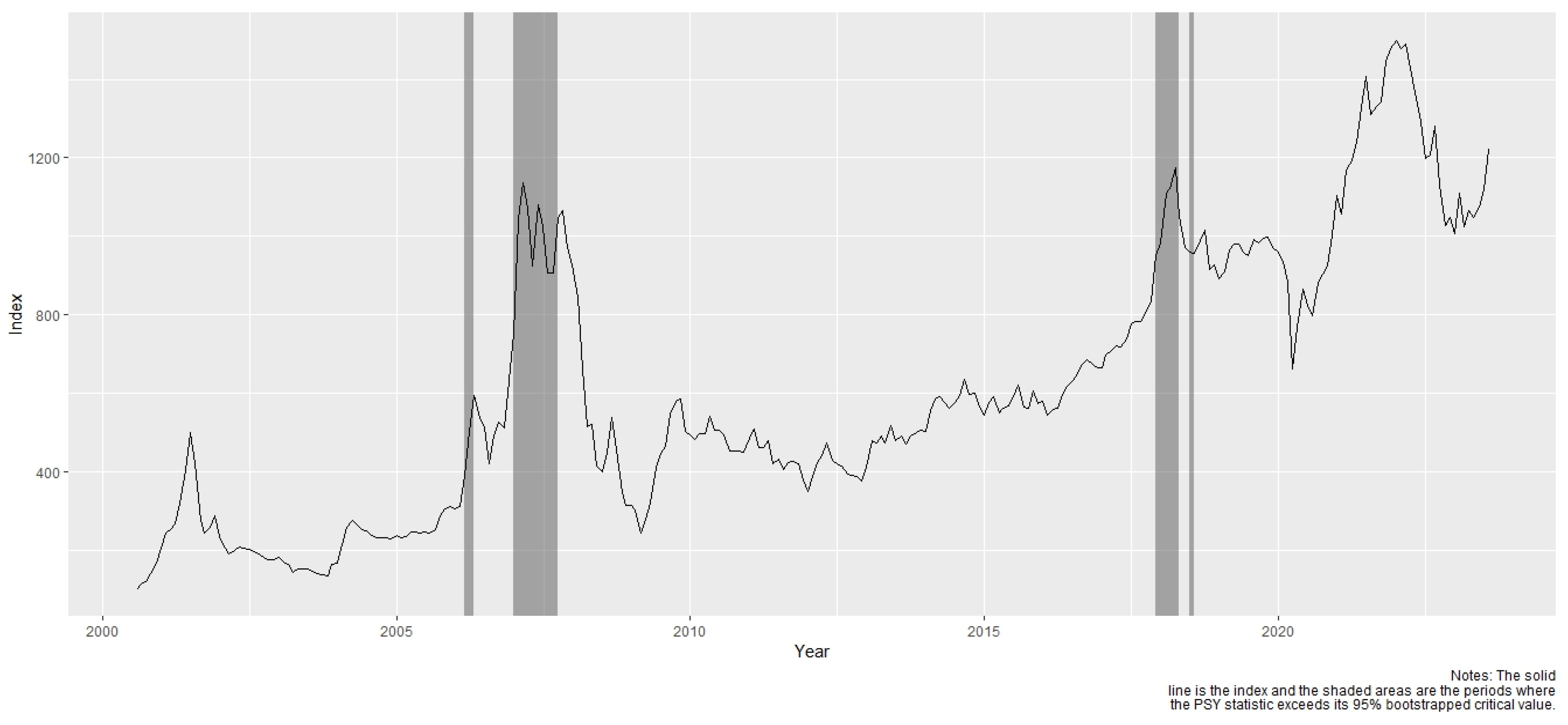
Table 1 displays the results of the financial bubble identification, providing the start and end dates for each bubble. The analysis identified a total of 33 months as having experienced financial bubbles, which are highlighted with dark gray vertical lines in Figure 2. Notably, two significant periods with multiple bubbles emerged during 2006–2007 and 2017–2018. These findings confirm the observations of financial experts regarding the overvaluation of stock prices in the stock market during these periods. Following the obtained results, we proceeded to label the months that were identified as bubbles, thereby preparing the dataset for the subsequent stage of supervised machine learning.
Table 2 presents the descriptive statistics of VNINDEX during the period with and without the presence of financial bubbles. It is evident from the table that the mean and quartile values of VNINDEX during the bubble period are higher as compared to the period without a bubble and also higher than the overall values, except for the maximum value.
5.2. Results of Forecasting Financial Bubbles Using Machine Learning Algorithms
Our study involved the implementation of various machine learning algorithms, including logistic regression, decision trees, random forest, neural networks, gradient boosting, and support vector machine (SVM).
We selected the hyperparameters based on the area under the ROC curve (AUC) to optimize the machine learning models. The AUC assesses a model’s classification performance by quantifying the area under the receiver operating characteristic (ROC) curve. In this process, a range of hyperparameter values is tested to fine-tune the model. The model is trained, and the AUC is calculated on the test dataset. The hyperparameter combination that yields the highest AUC is selected as optimal. This approach ensures that hyperparameters are chosen based on the model’s classification performance, with AUC serving as a key metric.
The following table summarizes the performance of these models.
The results in Table 3 show that both the random forest and neural network models outperform other algorithms in terms of AUC, accuracy, and F1 score. The neural network model stands out with the highest AUC (0.968), accuracy (0.915), and sensitivity (1.00), indicating its proficiency in accurately classifying periods marked by financial bubbles. However, the relatively lower F1 score (0.75) suggests a potential trade-off between precision and recall. This observation implies that, while the neural network excels in correctly classifying positive instances, it may benefit from adjustments to maintain a balance between precision and recall.
Additionally, the random forest algorithm delivers commendable results with a high AUC (0.953) and perfect precision (1.00), indicating its capacity to identify periods marked by financial bubbles precisely. However, its slightly lower sensitivity (0.667) implies a higher likelihood of missing some actual instances of financial bubbles. This trade-off underscores the need to consider the practical implications of false positives and false negatives in real-world financial decision-making. decision trees underperformed in comparison, with an AUC of 0.82 and lower F1 scores. This serves as a baseline for evaluating the machine learning models’ performance.
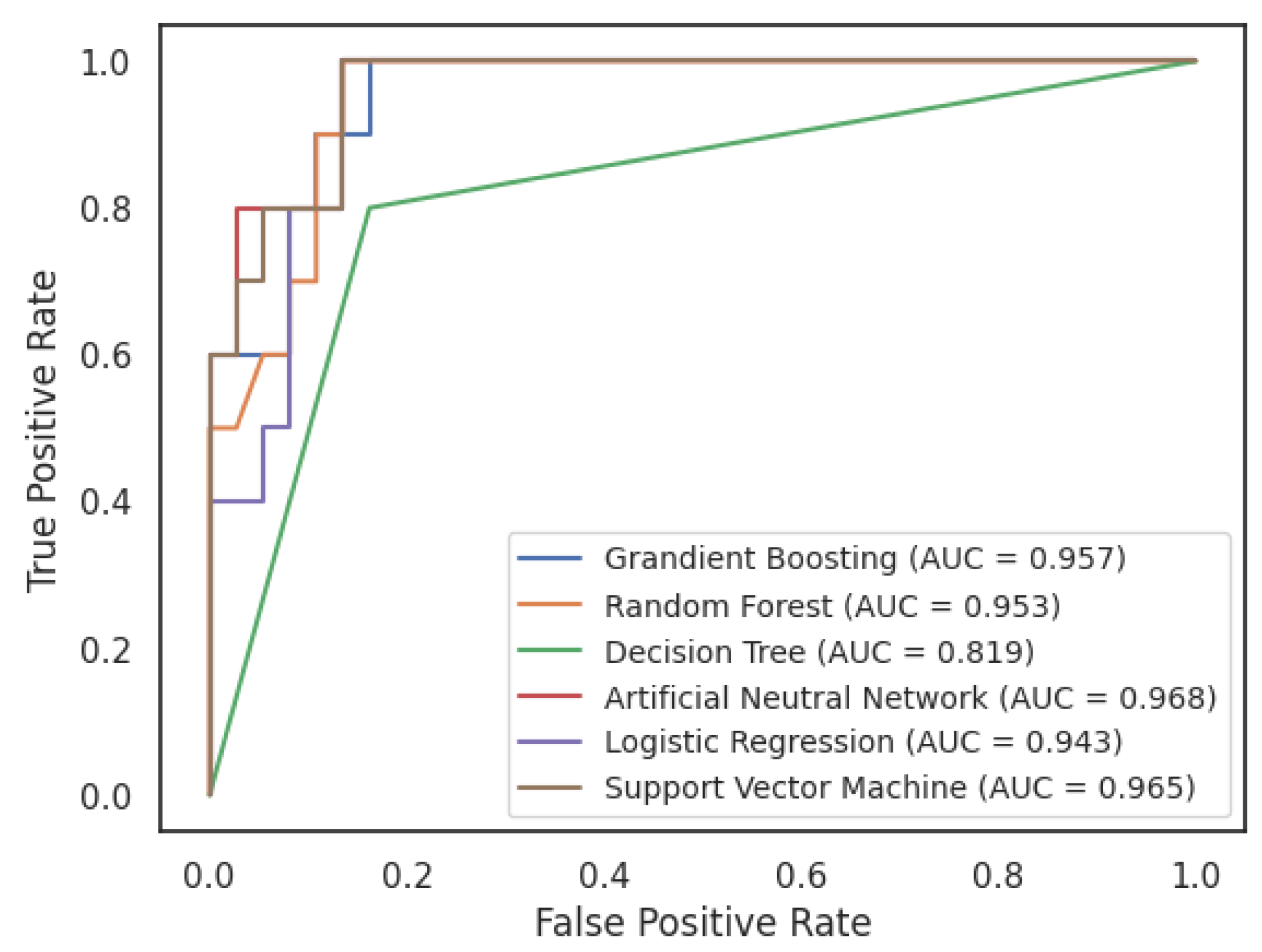
The Figure 3 also provided similar outcomes. Among the machine learning algorithms we employed, artificial neural network emerged as the top-performing model with an AUC score of 0.968. This score reflects its ability to achieve a high true positive rate while keeping the false positive rate low. In essence, it excels at distinguishing bubble periods from non-bubble periods in the stock market. Other models, including logistic regression and decision trees, demonstrated competitive but relatively lower AUC scores. While these models may still provide useful insights, their performance fell slightly behind that of neural networks, random forest, gradient boosting, and SVM in this specific task.
Based on the results, we compared the outcomes of machine learning methods with traditional statistical models. Models such as logistic regression, decision trees, and support vector machines are common methods in addressing classification problems in finance. The results suggest that advanced machine learning methods, particularly neural networks, random forest, and gradient boosting, outperformed the conventional methods (logistic regression, support vector machine, and decision trees) in terms of AUC, F1 score, and accuracy. This implies that machine learning models have the potential to better capture the complex patterns associated with financial bubbles.
In addition, it is essential to acknowledge that machine learning models can be sensitive to hyperparameters and the quality of training data, although proper tuning and regularization can enhance their robustness. On the other hand, conventional methods tend to offer greater robustness, especially when they are grounded in well-established economic theories and feature transparent model structures.
Regarding the aspect of explainability, machine learning models, such as neural networks, are often criticized for their perceived lack of interpretability, primarily due to their complex, black-box nature. Conventional methods are generally more interpretable due to their reliance on economic theories and transparent model structures. This makes it easier to explain the factors behind predictions. For further research, techniques like feature importance analysis, local interpretability methods, and documentation of the machine learning process can be applied to enhance the transparency and comprehensibility of these machine learning models. The choice between machine learning and conventional methods should consider the specific goals of the analysis and the need for transparency in explaining predictions to stakeholders or regulators. Combining both approaches, where machine learning enhances predictive performance and conventional methods provide explainability, may offer a balanced strategy for forecasting financial bubbles.
Our research results differ from the findings of Başoğlu Kabran and Ünlü (2021), which demonstrated that SVM yielded the best forecasting results for the S&P 500 index in the United States. We attribute this discrepancy to differences in the selected features incorporated into the models, as well as variations in the scale of the datasets used in the two studies. However, it is noteworthy that this study represents the first attempt to apply machine learning to forecast bubbles in an emerging market. In the future, we plan to conduct empirical research across a broader range of markets.
5.3. Robustness Test
To ensure the accuracy and reliability of the machine learning model, we conducted a robustness test by dividing the data into three equal parts: from September 2001 to February 2007, from March 2007 to August 2012, and from June 2014 to December 2019. The reason behind this is that all three periods have witnessed financial bubbles. We utilized two primary machine learning models—neural network and random forest—to predict financial bubbles for each data subset, and then trained and tested each model on their respective data subset. We evaluated the model performance using various metrics such as accuracy, the area under the ROC curve (AUC), and F1 score. Additionally, a PCA was employed to reduce data dimensionality and noise. Finally, we analyzed the results of all robustness test segments to compare the model performance across different time periods.
Table 4 shows that the AUC and accuracy values remained stable across all three periods, with average values of 0.935 and 0.842 for the neural network model and 0.951 and 0.883 for the random forest model, respectively. However, the sensitivity of the neural network model was found to be sensitive to the dataset, with a noticeable decrease in the period from June 2014 to December 2019. In contrast, the random forest model exhibited a higher stability in sensitivity values.
This robustness check method ensured the reliability of the financial bubble prediction model and provided a clear understanding of the model’s performance variation over time. It can help to make practical decisions regarding its application in the financial field.
5.4. Limitations and Future Research
While machine learning has demonstrated potential in forecasting financial bubbles in the stock market, its practical application may face various limitations. The first challenge is the interpretability of advanced machine learning models. Although such models deliver high accuracy, they often lack interpretability compared to traditional methods, like logistic regression. This can undermine the trust of policy makers and investors when using such models for critical decisions. Secondly, the Vietnamese stock market faces transparency issues in providing financial information and market events, which makes it difficult to obtain reliable input data for model development. Finally, the relatively young nature of the Vietnamese stock market limits the amount of available data for forecasting, which can affect the accuracy of predictions.
In terms of future research, subsequent studies can apply the methods used in this research to predict bubbles in other markets, such as real estate markets, commodity markets, and cryptocurrency markets. Another potential research avenue is to explore the relationship of financial bubbles between different markets, such as the stock market and real estate market, as macroeconomic factors heavily influence both. Understanding the interplay between markets enables regulatory authorities to implement policies to prevent the early formation of financial bubbles and create a healthy investment environment. A limitation of this research is the limited explanatory power of the machine learning models. Therefore, future studies may focus on improving the interpretability of machine learning models, thereby enhancing understanding and knowledge in this field.
6. Conclusions
In this study, we employed the PSY procedure to identify the presence of financial bubbles and forecast this phenomenon in the Vietnamese stock market using data from 2001 to 2021. The results indicate that financial bubbles occurred from 2006 to 2007 and 2017 to 2018. Regarding the predictive results, the neural network and random forest models exhibited a superior forecasting performance, with high F1 scores of 0.80 and 0.75, respectively. Based on the study’s findings, policymakers, governments, and market regulatory agencies have a valuable tool to detect and predict the emergence of financial bubbles on the real-time basis, enabling them to formulate appropriate policies to mitigate their adverse effects. From an academic perspective, this research also opens up potential avenues for applying machine learning tools to prediction tasks in the field of economics.
The study makes significant contributions to both theory and practice, providing empirical evidence of the applicability of machine learning in predicting financial bubbles in emerging markets like Vietnam. The research highlights the potential of random forest and artificial neural network as promising algorithms that can be effectively applied in the financial domain. For policymakers and regulators, the study underscores the importance of implementing timely policies to mitigate the likelihood and consequences of financial bubbles. The findings provide central banks and regulatory bodies with better tools to formulate appropriate monetary policies and regulate the flow of capital in the economy, thereby reducing speculative behavior in the prices of financial assets and ensuring stability in the financial system. The research also suggests that investors can benefit from the ability to predict price bubbles by choosing more effectively when to go long or short on assets, thus protecting their investment portfolios. Furthermore, bubbles represent opportunities for arbitrageurs to exploit by selling assets in overpriced markets, potentially yielding short-term profits.
Author Contributions
D.T.N. conceived the idea and wrote the Introduction. H.A.L. wrote the literature review. K.L.T. and C.P.L. wrote the methodology, results and discussion, and conclusions. All authors have read and agreed to the published version of the manuscript.
Funding
The research topic was supported by The Youth Incubator for Science and Technology Programme, managed by Youth Promotion Science and Technology Center–Ho Chi Minh Communist Youth Union and Department of Science and Technology of Ho Chi Minh City. The contract number is “25/2022/HĐ-KHCNT-VU” signed on 30 December 2022.
Data Availability Statement
The data for this study can be found on our GitHub page: https://github.com/kimlongdhnh/long.tran.git (accessed on 2 September 2022).
Conflicts of Interest
The authors declare no conflict of interest.
References
- Alessi, Lucia, and Carsten Detken. 2018. Identifying excessive credit growth and leverage. Journal of Financial Stability 35: 215–25. [Google Scholar] [CrossRef]
- Barboza, Flavio, Herbert Kimura, and Edward Altman. 2017. Machine learning models and bankruptcy prediction. Expert Systems with Applications 83: 405–17. [Google Scholar] [CrossRef]
- Başoğlu Kabran, Fatma, and Kamil Demirberk Ünlü. 2021. A two-step machine learning approach to predict S&P 500 bubbles. Journal of Applied Statistics 48: 2776–94. [Google Scholar] [PubMed]
- Beutel, Johannes, Sophia List, and Gregor von Schweinitz. 2019. Does machine learning help us predict banking crises? Journal of Financial Stability 45: 100693. [Google Scholar] [CrossRef]
- Breiman, Leo. 2001. Random forests. Machine learning 45: 5–32. [Google Scholar] [CrossRef]
- Cakici, Nusret, Christian Fieberg, Daniel Metko, and Adam Zaremba. 2023. Do Anomalies Really Predict Market Returns? New Data and New Evidence. Review of Finance. Forthcoming. [Google Scholar] [CrossRef]
- Case, Karl E., and Robert J. Shiller. 2003. Is there a bubble in the housing market? Brookings Papers on Economic Activity 2003: 299–362. [Google Scholar] [CrossRef]
- Chatzis, Sotirios P., Vassilis Siakoulis, Anastasios Petropoulos, Evangelos Stavroulakis, and Nikos Vlachogiannakis. 2018. Forecasting stock market crisis events using deep and statistical machine learning techniques. Expert Systems with Applications 112: 353–71. [Google Scholar] [CrossRef]
- Dong, Xi, Yan Li, David E. Rapach, and Guofu Zhou. 2022. Anomalies and the expected market return. The Journal of Finance 77: 639–81. [Google Scholar] [CrossRef]
- Fama, Eugene F. 2014. Two pillars of asset pricing. American Economic Review 104: 1467–85. [Google Scholar] [CrossRef]
- Fuster, Andreas, Paul Goldsmith-Pinkham, Tarun Ramadorai, and Ansgar Walther. 2022. Predictably unequal. The Effects of Machine Learning on Credit Markets. Journal of Finance 77: 1–808. [Google Scholar] [CrossRef]
- Galbraith, James K., Sara Hsu, and Wenjie Zhang. 2009. Beijing bubble, Beijing bust: Inequality, trade, and capital inflow into China. Journal of Current Chinese Affairs 38: 3–26. [Google Scholar] [CrossRef]
- Geng, Ruibin, Indranil Bose, and Xi Chen. 2015. Prediction of financial distress: An empirical study of listed Chinese companies using data mining. European Journal of Operational Research 241: 236–47. [Google Scholar] [CrossRef]
- Gu, Shihao, Bryan Kelly, and Dacheng Xiu. 2020. Empirical asset pricing via machine learning. The Review of Financial Studies 33: 2223–73. [Google Scholar] [CrossRef]
- Harris, Charles R., K. Jarrod Millman, Stéfan J. Van Der Walt, Ralf Gommers, Pauli Virtanen, David Cournapeau, Eric Wieser, Julian Taylor, Sebastian Berg, and Nathaniel J. Smith. 2020. Array programming with NumPy. Nature 585: 357–62. [Google Scholar] [CrossRef]
- Homm, Ulrich, and Jörg Breitung. 2012. Testing for speculative bubbles in stock markets: A comparison of alternative methods. Journal of Financial Econometrics 10: 198–231. [Google Scholar] [CrossRef]
- Kindleberger, Charles Poor, Robert Z. Aliber, and Robert M. Solow. 2005. Manias, Panics, and Crashes: A History of Financial Crises. London: Palgrave Macmillan London, vol. 7. [Google Scholar]
- McKinney, Wes. 2010. Data structures for statistical computing in python. Paper presented at the 9th Python in Science Conference, Austin, TX, USA, June 28–July 3. [Google Scholar]
- Ouyang, Zi-sheng, and Yongzeng Lai. 2021. Systemic financial risk early warning of financial market in China using Attention-LSTM model. The North American Journal of Economics and Finance 56: 101383. [Google Scholar] [CrossRef]
- Pedregosa, Fabian, Gaël Varoquaux, Alexandre Gramfort, Vincent Michel, Bertrand Thirion, Olivier Grisel, Mathieu Blondel, Peter Prettenhofer, Ron Weiss, and Vincent Dubourg. 2011. Scikit-learn: Machine learning in Python. The Journal of Machine Learning Research 12: 2825–30. [Google Scholar]
- Phillips, Peter C. B., Shuping Shi, and Jun Yu. 2015a. Testing for multiple bubbles: Limit theory of real-time detectors. International Economic Review 56: 1079–134. [Google Scholar] [CrossRef]
- Phillips, Peter C. B., Shuping Shi, and Jun Yu. 2015b. Testing for multiple bubbles: Historical episodes of exuberance and collapse in the S&P 500. International Economic Review 56: 1043–78. [Google Scholar]
- Phillips, Peter C. B., Shuping Shi, Itamar Caspi, and Maintainer Itamar Caspi. 1984. Package ‘psymonitor’. Biometrika 71: 599–607. [Google Scholar]
- Phillips, Peter C. B., Yangru Wu, and Jun Yu. 2011. Explosive behavior in the 1990s Nasdaq: When did exuberance escalate asset values? International Economic Review 52: 201–26. [Google Scholar] [CrossRef]
- Shiller, Robert J. 1981. Do stock prices move too much to be justified by subsequent changes in dividends? The American Economic Review 71: 421–436. [Google Scholar]
- Shiller, Robert J. 2002. Bubbles, human judgment, and expert opinion. Financial Analysts Journal 58: 18–26. [Google Scholar] [CrossRef]
- Shiller, Robert J. 2015. Irrational Exuberance. Princeton: Princeton University Press. [Google Scholar]
- Shin, Kyung-Shik, Taik Soo Lee, and Hyun-jung Kim. 2005. An application of support vector machines in bankruptcy prediction model. Expert Systems with Applications 28: 127–35. [Google Scholar] [CrossRef]
- Stiglitz, Joseph E. 1990. Symposium on bubbles. Journal of Economic Perspectives 4: 13–18. [Google Scholar] [CrossRef]
- Tirole, Jean. 2008. Liquidity shortages: Theoretical underpinnings. Financial Stability Review 11: 53–63. [Google Scholar]
- Tran, Kim Long, Hoang Anh Le, Thanh Hien Nguyen, and Duc Trung Nguyen. 2022. Explainable machine learning for financial distress prediction: Evidence from Vietnam. Data 7: 160. [Google Scholar] [CrossRef]
- Waskom, Michael, Olga Botvinnik, Drew O’Kane, Paul Hobson, Saulius Lukauskas, David C. Gemperline, Tom Augspurger, Yaroslav Halchenko, John B. Cole, and Jordi Warmenhoven. 2017. Mwaskom/Seaborn: V0. 8.1 (September 2017). Zenodo. Available online: https://github.com/mwaskom/seaborn/tree/v0.8.1 (accessed on 24 September 2023).
- West, Kenneth D. 1987. A specification test for speculative bubbles. The Quarterly Journal of Economics 102: 553–80. [Google Scholar] [CrossRef]
- Zhao, Zongyuan, Shuxiang Xu, Byeong Ho Kang, Mir Md Jahangir Kabir, Yunling Liu, and Rainer Wasinger. 2015. Investigation and improvement of multi-layer perceptron neural networks for credit scoring. Expert Systems with Applications 42: 3508–16. [Google Scholar] [CrossRef]
- Zhou, Xianzheng, Hui Zhou, and Huaigang Long. 2023. Forecasting the equity premium: Do deep neural network models work? Modern Finance 1: 1–11. [Google Scholar] [CrossRef]
Figure 1.
Explained variance plot. Source: authors (2023).

Figure 2.
Bubbles in the Vietnam Stock market from January 2001 to December 2021.

Figure 3.
ROC curve of the classifiers.


Table 1.
Statistics of financial bubbles occurrences.
| Start Date | End Date | |
|---|---|---|
| 1 | 28 February 2006 | 28 April 2006 |
| 2 | 30 June 2006 | 30 June 2006 |
| 3 | December 2006 | 28 September 2007 |
| 4 | November 2017 | 27 April 2018 |
| 5 | 29 June 2018 | 31 July 2018 |
Source: authors (2023).
Table 2.
Descriptive statistics of VNINDEX.
| Bubble Months | Non-Bubble Months | Overall | |
|---|---|---|---|
| count | 33 | 218 | 251 |
| mean | 896.70 | 524.54 | 573.47 |
| std | 220.47 | 286.81 | 305.78 |
| min | 401.90 | 135.78 | 135.78 |
| 25% | 842.71 | 291.25 | 320.92 |
| 50% | 975.94 | 489.06 | 514.92 |
| 75% | 1049.32 | 631.40 | 782.85 |
| max | 1196.61 | 1478.44 | 1478.44 |
Source: authors (2023).
Table 3.
The performance results of classifiers.
| Algorithms | Hyperparameter | AUC | F1 Score | Accuracy | Precision | Sensitivity |
|---|---|---|---|---|---|---|
| Neural Networks | hidden_layer_sizes = 100, max_iter = 300, activation = “relu”, solver = ‘adam’, alpha = 0.0001 | 0.968 | 0.750 | 0.915 | 0.600 | 1.000 |
| Random Forest | max_depth = 5, n_estimators = 50 | 0.953 | 0.800 | 0.894 | 1.000 | 0.667 |
| Gradient Boosting | max_depth = 3, learning_rate = 0.1, n_estimators = 100 | 0.957 | 0.727 | 0.872 | 0.800 | 0.667 |
| Logistic Regression | C = 1 | 0.943 | 0.700 | 0.872 | 0.700 | 0.700 |
| Support Vector Machine | C = 1, kernel = ‘rbf’, class_weight = ‘balanced’ | 0.965 | 0.696 | 0.851 | 0.800 | 0.615 |
| Decision Trees | max_depth = 5 | 0.819 | 0.667 | 0.830 | 0.800 | 0.571 |
Source: authors (2023).
Table 4.
The robustness test results.
| Neural Network | Random Forest | |||||||
|---|---|---|---|---|---|---|---|---|
| September 2001–February 2007 | March 2007–August 2012 | June 2014–December 2019 | Average | September 2001–February 2007 | March 2007–August 2012 | June 2014–December 2019 | Average | |
| Accuracy | 0.950 | 0.950 | 0.905 | 0.935 | 0.950 | 0.950 | 0.952 | 0.951 |
| AUC | 0.875 | 0.900 | 0.750 | 0.842 | 0.875 | 0.900 | 0.875 | 0.883 |
| Sensitivity | 0.750 | 0.800 | 0.500 | 0.683 | 0.750 | 0.800 | 0.750 | 0.767 |
Source: authors (2023).
Disclaimer/Publisher’s Note: The statements, opinions and data contained in all publications are solely those of the individual author(s) and contributor(s) and not of MDPI and/or the editor(s). MDPI and/or the editor(s) disclaim responsibility for any injury to people or property resulting from any ideas, methods, instructions or products referred to in the content. |
© 2023 by the authors. Licensee MDPI, Basel, Switzerland. This article is an open access article distributed under the terms and conditions of the Creative Commons Attribution (CC BY) license (https://creativecommons.org/licenses/by/4.0/).
Share and Cite
MDPI and ACS Style
Tran, K.L.; Le, H.A.; Lieu, C.P.; Nguyen, D.T. Machine Learning to Forecast Financial Bubbles in Stock Markets: Evidence from Vietnam. Int. J. Financial Stud. 2023, 11, 133. https://doi.org/10.3390/ijfs11040133
AMA Style
Tran KL, Le HA, Lieu CP, Nguyen DT. Machine Learning to Forecast Financial Bubbles in Stock Markets: Evidence from Vietnam. International Journal of Financial Studies. 2023; 11(4):133. https://doi.org/10.3390/ijfs11040133
Chicago/Turabian StyleTran, Kim Long, Hoang Anh Le, Cap Phu Lieu, and Duc Trung Nguyen. 2023. "Machine Learning to Forecast Financial Bubbles in Stock Markets: Evidence from Vietnam" International Journal of Financial Studies 11, no. 4: 133. https://doi.org/10.3390/ijfs11040133
Note that from the first issue of 2016, this journal uses article numbers instead of page numbers. See further details here.