The Impact of Monetary Policy on the U.S. Stock Market since the COVID-19 Pandemic

Abstract

Inflation in 2021 and 2022 grew much faster than the Federal Reserve expected. The Fed downplayed inflation in 2021 and then increased the federal funds rate by 500 basis points between March 2022 and May 2023. This paper investigates how this unprecedented tightening has impacted the stock market. To do so, it estimates a fully specified multi-factor model that measures the exposure of 53 assets to monetary policy surprises over the 1994 to 2019 period. It then uses the monetary policy betas to gauge investors’ beliefs about monetary policy between 2020 and 2023. The results indicate that changing perceptions about monetary policy multiplied uncertainty and stock market volatility.

1. Introduction

News about COVID-19, inflation, and monetary policy has buffeted the U.S. economy since 2020. As the pandemic emerged, the Federal Reserve lowered its target for the federal funds rate by 150 basis points in March 2020. The year-on-year change in the U.S. consumer price index (CPI) then rose from 1.5% in March 2020 to 8.6% in June 2022. The Fed raised its funds rate target by 500 basis points in 2022 and 2023. This paper investigates how monetary policy news has impacted the stock market since the coronavirus crisis began.

The Fed responded to the pandemic not only by lowering the funds rate but also by providing forward guidance that interest rates would remain low, purchasing Treasury and mortgage-backed securities, lending to Treasury security primary dealers, backstopping money market funds, and encouraging bank lending and credit extension.1 The government provided three rounds of stimulus checks. These policies increased demand, while negative shocks associated with the pandemic, value chain disruptions, and the Russia-Ukraine War restricted supply.

This combination contributed to inflation that proved higher and more persistent than the Fed expected. At the end of 2020, the median forecast of Federal Reserve Board members and Federal Reserve Bank presidents was that the personal consumption expenditures (PCE) price index would grow by 1.8% between 2020Q4 and 2021Q4. It actually grew by 5.7%. At the end of 2021, the median forecast was for the PCE index to grow by 2.6% between 2021Q4 and 2022Q4. It again grew by 5.7%.2 In November 2021, Fed Chair Jerome Powell stopped calling inflation transitory, and in 2022, the Fed began aggressively raising the funds rate.

Previous work has investigated the interaction between monetary policy, inflation, and asset prices after the pandemic. Gagliardone and Gertler (2023) examined the role of easy monetary policy and oil shocks in explaining the inflation surge that began in 2021. They employed a New Keynesian model with oil included as both a consumption good and an input into production. Their model assumed real wage rigidity and allowed for unemployment. They derived key parameters by matching the model’s impulse responses to those obtained from a structural vector autoregression (VAR). They reported that the inflation that emerged in 2021 arose from a combination of easy monetary policy (i.e., the delayed response of the Fed to increasing inflation in 2021) and oil price shocks.

Bernanke and Blanchard (2023) also investigated the causes of inflation after 2019. They employed a model where nominal wages depend on labor market slack, prices depend on nominal wages and other input costs, and expected inflation depends on last period’s expected inflation and on current inflation. They used their model to impose contemporaneous restrictions on a structural VAR that they estimated over the 1990Q1–2019Q4 period. They found that commodity price hikes and relative price increases due to supply shocks led to the inflation that began in 2021. They reported that, up to 2023, labor market tightness caused only a little inflation.

Eggertsson and Kohn (2023) examined whether the policy framework (PF) that the Fed implemented in 2020 contributed to the inflation surge that started in 2021. They noted that the Fed in 2020 adopted an asymmetric loss function whereby it was less willing to tighten when employment exceeded its “maximum” level than it was to ease when employment fell short of this level. They presented narrative evidence that the new PF caused the Fed to delay tightening as inflation emerged in 2021. They argued that an earlier response would have promoted financial stability by enabling the Fed to tighten more gradually.

Chibane and Kuhanathan (2023), using inflation swap data, found that the probability of a non-Gaussian jump in U.S. inflation swaps doubled beginning in the third quarter of 2020. They investigated whether Fed policy was subsequently able to re-anchor inflation expectations. They used both an event study of Federal Open Market Committee (FOMC) meetings and short-term interest rates to measure monetary policy. Their data extended to September 2022. They reported that news of contractionary monetary policy did not reduce the probability of jumps in U.S. inflation swaps. They concluded that contractionary monetary policy up to September 2022 had failed to re-anchor inflation expectations.

Adams et al. (2023) measured financial market sentiment by applying language processing techniques to Twitter data. They reported that an unexpected tightening of monetary policy worsens sentiment. They found that sentiment worsened in September 2021, when Fed communication pivoted towards a tightening cycle.

Dietrich et al. (2022) employed a daily survey of consumers’ expectations during the pandemic. They received 60,000 responses. They reported that consumers expected the pandemic to have a stagflationary effect. They also found that the pandemic caused huge uncertainty to consumers about the future path of inflation. Calibrating the consumers’ responses using a business cycle model, they concluded that better communication by the central bank to the broader public could have mitigated uncertainty and dampened the resulting shocks.

Arteta et al. (2022) investigated the factors affecting U.S. 2-year and 10-year Treasury bond yields in 2022. They employed a sign-restricted Bayesian VAR using monthly data on 2-year and 10-year Treasury bond yields, the S&P 500 index, and inflation expectations over the January 1982 to June 2022 period. They reported that changing perceptions of the Fed’s reaction function, whereby investors inferred the Fed’s changing attitudes towards inflation, explained much of the change in Treasury bond yields in 2022.

Several papers have also highlighted how uncertainty about macroeconomic variables affects asset returns. Bernanke and Kuttner (2005), using a VAR and monthly data over the 1973–2002 period, found that easier monetary policy reduces the risk premium that investors require to hold stocks.3 Hanson and Stein (2015), using data on forward interest rates and monthly data over the 1987–2012 period, presented evidence supporting the hypothesis that monetary policy affects the term premium on long-term bonds. Kashyap and Stein (2023), surveying many studies, reported that expansionary monetary policy lowers risk premia on stocks, Treasury securities, corporate bonds, and foreign exchange rates.

Chen et al. (1986) (CRR), using monthly data over the 1958 to 1984 period, found that assets that are harmed by unexpected increases in inflation must pay higher expected returns. Bekaert and Wang (2010), reviewing the literature, found that studies employing inflation-linked bonds and inflation surveys reported positive risk premia for assets exposed to inflation. Cieslak and Pflueger (2023), comparing survey inflation expectations with inflation swap rates over the 2004–2023 period, reported that inflation risk premia are often negative over the following three quarters and positive over the following ten years.

This paper investigates how monetary policy has impacted financial markets since the pandemic began. To do this, it first estimates a multi-factor model including news about monetary policy and other macroeconomic variables over the 1994 to 2019 period. It then uses assets’ monetary policy betas to examine how investors responded to news about monetary policy beginning in 2020. If investors anticipated contractionary monetary policy, this would cause the prices of assets that are harmed by contractionary monetary policy to fall and the prices of assets that benefit to rise.

The estimated monetary policy betas indicate that monetary policy matters for many stocks. The results also indicate that changing perceptions about monetary policy caused large swings in U.S. equity prices in 2022. Going forward, central bankers should consider how they can reduce financial market volatility associated with uncertainty about monetary policy. One way would be to recognize incipient inflation quickly, rather than waiting until inflation becomes entrenched and then resorting to a monetary policy sledgehammer. Another way would be to clearly communicate the Fed’s preferences towards inflation.

The next section presents the data and methodology. Section 3 presents the results. Section 4 concludes.

2. Data and Methodology

The first goal of this paper is to estimate monetary policy betas in the context of a fully specified multi-factor asset pricing model. Ross (2001) demonstrated that in a multi-factor model, an asset’s expected return equals the return on the risk-free asset plus the inner product of a vector of assets’ betas to macroeconomic factors with a vector of risk prices:

$$E_i={\lambda }_0+{\displaystyle \sum }_{j=1}^K{\beta }_{ij}{\lambda }_j$$

(1)

where E_i is the ex-ante expected return on asset i, λ₀ is the return on the risk-free asset, β_ij is the beta or factor loading of asset i to macroeconomic factor j, and λ_j is the risk price associated with factor j. The ex-post realized return equals the sum of the expected return, a beta-weighted vector of unexpected changes in the macroeconomic factors, and an error term capturing the effects of idiosyncratic news:

$$R_i={\lambda }_0+{\displaystyle \sum }_{j=1}^K{\beta }_{ij}{\lambda }_j+{\displaystyle \sum }_{j=1}^K{\beta }_{ij}{f}_j+{\epsilon }_i$$

(2)

where R_i is the ex-post realized return, f_j represents news about macroeconomic factor j and ε_i is a mean-zero error term.

Gallant’s (1975) iterated nonlinear seemingly unrelated regression method (INLSUR) can be used to simultaneously estimate the factor loadings and the risk prices and to impose the nonlinear cross-equation restrictions that the intercept terms depend on the risk prices. This technique delivers consistent estimates of the betas and the risk prices. (See McElroy and Burmeister (1988)). Equation (2) can be stacked and the model estimated as a system using INLSUR:

$$\left[\begin{array}{c}{R}_1-{\lambda }_0\\ R_2-{\lambda }_0\\ .\\ .\\ .\\ R_n-{\lambda }_0\end{array}\right]=\left[\begin{array}{cccccc}X\left(\lambda ,f\right)& 0& .& .& .& 0\\ 0& X\left(\lambda ,f\right)& .& .& .& 0\\ 0& 0& .& .& .& 0\\ 0& 0& .& .& .& 0\\ 0& 0& .& .& .& 0\\ 0& 0& .& .& .& X\left(\lambda ,f\right)\end{array}\right]\left[\begin{array}{c}{\beta }_1\\ {\beta }_2\\ .\\ .\\ .\\ {\beta }_n\end{array}\right]+\left[\begin{array}{c}{\epsilon }_1\\ {\epsilon }_2\\ .\\ .\\ .\\ {\epsilon }_n\end{array}\right] .$$

(3)

R_i − λ₀ is a 1 × T vector where R_i represents the realized return on asset i and λ₀ is the return on the risk-free asset. X(λ,f) is a T × k matrix whose tith element equals f_it + λ_i. β_i is a 1 × k vector measuring asset i’s sensitivity to the macroeconomic factors. ε_i is an i×T vector, where by assumption E(ε₁, ε₂, …, ε_n) = 0_nT, E(ε₁, ε₂, …, ε_n)’(ε₁, ε₂, …, ε_n) = ∑⊗I_T, and ∑_i,j = cov(ε_i,t, ε_j,t).

CRR (1996) used observable macroeconomic data (not latent variables from a dynamic factor model) to measure the common factors. The factors they employed were the difference in returns between 20-year and one-month treasury securities (the horizon premium), the difference in returns between 20-year corporate bonds and 20-year treasury bonds (the default premium), the monthly growth rate in industrial production, unexpected inflation, and the change in expected inflation. CRR argued that each of these macroeconomic factors, being either the difference between asset returns or very noisy, can be treated as innovations. They also argued that, while only phenomena such as supernovas are truly exogenous, the macroeconomic variables on the right-hand side can be treated as exogenous relative to the portfolio returns on the left-hand side.

Thorbecke (2018) reported that the default premium was not a price factor. Thus, in this paper, the default premium is replaced by an indicator of monetary policy. The other variables are the same ones used by CRR.

Monetary policy is measured using the surprise monetary policy variables constructed by Bu et al. (2021) (BRW). BRW used Fama and MacBeth’s (1973) two-step regression approach and instrumental variable techniques to extract a monetary policy surprise series from the response of zero-coupon Treasury yields to monetary policy news. Their measure captures the impact of changes in the funds rate target, large-scale asset purchases, and forward guidance. It has large effects on yields in the middle of the term structure and generates correctly signed impulse responses for output and inflation. Their data begin in January 1994, so the sample period to estimate the multi-factor model extends from January 1994 to December 2019.4

Unexpected inflation, following Boudoukh et al. (1994), is calculated as the residuals from a regression of the monthly CPI inflation rate on lagged CPI inflation and current and lagged one-month Treasury bill returns. The change in expected inflation is also calculated from this model. The data to calculate the inflation factors and the horizon premium come from Kroll (2023). Data to calculate the growth rate of industrial production come from the Federal Reserve Bank of St. Louis FRED database.

Table 1. Correlation matrix for economic variables.

Variable	Unexpected Inflation	Horizon Premium	Change in Expected Inflation	Industrial Production Growth
Unexpected inflation
Horizon Premium	−0.215
Change in expected inflation	0.145	−0.156
Industrial production growth	−0.109	−0.018	0.056
Monetary policy (Bu et al. measure)	0.034	0.027	0.023	0.008

Note: The table presents correlation coefficients for the economic variables. Unexpected inflation is calculated as the residuals from a regression of the consumer price index inflation rate on lagged inflation and current and lagged Treasury bill returns. The change in expected inflation is also calculated from this model. The horizon premium is the difference between returns on 20-year and one-month Treasury securities. Industrial production growth is the monthly growth rate of industrial production. Monetary policy is measured using the Bu et al. (2021) Fed policy surprise variable.

presents a correlation matrix for the independent variables. The table indicates that multicollinearity is not a problem. It is noteworthy that the BRW monetary policy surprises are uncorrelated with the other variables.

The left-hand side variables include the excess returns (realized returns minus returns on one-month Treasury bills) on 53 assets. These assets are primarily returns on industry stock portfolios.5 However, since Frankel (2008) and others have found that commodities such as gold and silver can benefit from inflationary news, the returns on gold and silver are included. This increases the cross-sectional variation in expected returns. Data on the return on one-month Treasury bills come from Kroll (2023), and data on the other asset returns come from the Datastream database.6

The second goal of this paper is to use the monetary policy betas to investigate investors’ changing perceptions about monetary policy beginning in 2020. News of contractionary policy will push up the prices of assets that benefit from contractionary policy (those with larger betas to the BRW variable) and push down the prices of those that are harmed (those with smaller betas to the BRW variable). There should thus be a positive relationship between asset returns and assets’ BRW betas on months when investors foresee tighter monetary policy. Similarly, there should be a negative relationship between asset returns and assets’ BRW betas on months when investors foresee easier monetary policy. For each month from April 2020 to April 2023, returns on the 53 assets are thus regressed on the monetary policy betas estimated over the 1994–2019 period.

3. Results

Table 2. Iterated nonlinear seemingly unrelated regression estimates of the risk prices associated with macroeconomic factors.

(1)	(2)
Macroeconomic factor	Risk price
Unexpected inflation	−0.0029 ** (0.0014)
Horizon premium	−0.0105 * (0.0060)
Change in expected inflation	−0.0020 ** (0.0009)
Industrial production growth	−0.0127 *** (0.0043)
Monetary policy (Bu, Rogers, and Wu Measure)	−0.0368 ** (0.0178)

Note: The table presents iterated nonlinear seemingly unrelated regression estimates of risk prices from a multi-factor model, including returns on 53 assets (minus the return on one-month Treasury bills) on the left-hand side and unexpected inflation, the horizon premium (the difference between returns on 20-year and one-month Treasury securities), the change in expected inflation, the monthly growth rate in industrial production, and the Bu et al. (2021) (BRW) measure of Fed policy surprises on the right-hand side. Unexpected inflation is calculated as the residuals from a regression of the consumer price index inflation rate on lagged inflation and current and lagged Treasury bill returns. The change in expected inflation is also calculated from this model. The BRW measure is constructed so that an increase represents a contractionary monetary policy surprise. The sample extends from January 1994 to December 2019. *** (**) [*] denotes significance at the 1% (5%) [10%] level.

presents the risk prices from estimating the multi-factor model. Column (2) presents the risk price and column (3) presents the standard errors. For unexpected inflation, the risk price is statistically significant and equals −0.0029. To understand how this risk price impacts the risk premium, consider the inflation beta for airlines, which equals −2.85. This beta can be viewed as the quantity of inflation risk associated with the airlines sector. Multiplying the inflation risk price (−0.0029) by the quantity of inflation risk (−2.85), the inflation risk premium associated with airlines is 0.0083. This implies that the required return to hold airline stocks increases by 0.83% per month because airline stocks perform badly when unexpected inflation increases. On the other hand, the estimated inflation beta for silver is 4.71. Multiplying the risk price by the quantity of inflation risk, the risk premium associated with silver is −0.0177. This implies that the required return to hold silver decreases by 1.77% per month because silver does well when unexpected inflation increases.

Bekaert and Wang (2010) reported positive risk premia for assets that are harmed by higher inflation. Cieslak and Pflueger (2023), on the other hand, found that inflation risk premia are often negative over the following three quarters. The results here are consistent with Bekaert and Wang’s (2010) findings that assets exposed to inflation must pay a positive increment to their required returns.

For the horizon premium, the risk price in Table 2 equals −0.0105 and is statistically significant at the 10% level. The horizon premium measures the difference in returns between 20-year and one-month Treasury securities. It is closely related to the spread between long-term and short-term interest rates. A decrease in this spread helps predict a recession (see, e.g., Hornstein 2022). A decrease in the long-term interest rate would cause a capital gain for those holding long-term bonds and thus increase the horizon premium. So, an increase in the horizon premium is associated with a decrease in the long/short interest rate spread.

For sectors more exposed to decreases in the interest rate spread (those with negative betas to the horizon premium), the risk price in Table 2 implies that they would have to pay higher expected returns. For instance, for the automobile sector, the horizon premium beta equals −0.604. Automobile stocks would thus have to pay a risk premium of −0.0105 × −0.604 = 0.0063. Thus, automobile stocks would have to pay a positive premium of 0.63% per month to compensate for their exposure to decreases in the interest rate spread. On the other hand, the electricity sector is less cyclically sensitive, and its horizon premium beta equals 0.234. Electricity stocks would thus have a required return of 0.43% less per month because they do well when the horizon premium increases.

The risk prices associated with the change in expected inflation, industrial production growth, and monetary policy are statistically significant. For monetary policy, the risk price equals −0.0368. For sectors exposed to contractionary monetary policy (those with negative monetary policy betas), the risk price implies that they would have to pay higher expected returns. For instance, for the aluminum sector, the monetary policy beta equals −0.438. Aluminum stocks would thus have to pay a positive premium of 1.61% per month to compensate for their exposure to contractionary monetary policy. On the other hand, sectors such as food retailers and wholesalers that are not exposed to monetary policy would not have to pay a premium to compensate for monetary policy risk.

Table 3. Iterated nonlinear seemingly unrelated regression estimates of assets’ sensitivities to Bu et al. (2021) Fed policy surprises.

(1)	(2)	(3)
Asset	Monetary Policy Beta (Bu, Rogers, and Wu Measure)	Standard Error
Aerospace/defense	−0.109	0.081
Aerospace	−0.141	0.089
Airlines	−0.056	0.129
Aluminum	−0.438 **	0.198
Apparel retail	−0.123	0.110
Auto and parts	−0.077	0.114
Auto parts	−0.034	0.099
Automobiles	−0.091	0.142
Basic materials	−0.297 ***	0.087
Basic resources	−0.397 ***	0.113
Beverages	−0.043	0.068
Broadcast and entertainment	−0.100	0.095
Brewers	−0.023	0.084
Building materials/fixtures	−0.068	0.093
Business supply services	−0.094	0.077
Chemicals	−0.274 ***	0.080
Clothing and accessories	−0.187 *	0.102
Commercial vehicles/trucks	−0.259 **	0.110
Computer hardware	−0.239 **	0.116
Computer services	−0.130 *	0.079
Construction and materials	−0.239 **	0.093
Consumer electricity	−0.069	0.063
Consumer discretionary	−0.140 **	0.069
Consumer finance	−0.160 *	0.097
Consumer goods	−0.078	0.069
Consumer staples	−0.038	0.054
Consumer services	−0.136 **	0.069
Container and packaging	−0.181 **	0.086
Defense	−0.057	0.087
Distillers and vintners	−0.016	0.083
Diversified industrials	−0.068	0.088
Drug retailers	−0.098	0.092
Durable household products	−0.201 *	0.120
Electronic components and equipment	−0.228 **	0.094
Electricity	−0.070	0.063
Electronic and electrical equipment	−0.218 **	0.095
Food and drug retail	−0.077	0.066
Food producers	−0.073	0.056
Food retailers and wholesalers	−0.019	0.073
Financial services	−0.204 **	0.086
Financials	−0.130	0.082
Gold Bullion	−0.129 **	0.063
Gold mining (Americas)	−0.190	0.148
Gold mining (Australasia)	−0.318 *	0.164
Gold mining (World)	−0.200	0.140
Health care	−0.088	0.058
Oil and gas	−0.200 **	0.080
Pharmaceuticals and biochemical products	−0.051	0.066
Real estate investment trusts	−0.019	0.083
Silver (S&P GSCI)	−0.411 ***	0.118
Technology	−0.172	0.106
Telecom	−0.074	0.080
Utilities	−0.063	0.062

Note: The table presents iterated nonlinear seemingly unrelated regression estimates of assets’ betas to the Bu et al. (2021) (BRW) measure of Fed policy surprises from a multi-factor model that includes returns on the 53 assets listed in column (1) (minus the return on one-month Treasury bills) on the left-hand side and the difference between returns on 20-year and one-month Treasury securities, the BRW measure, the monthly growth rate in industrial production, unexpected inflation, and the change in expected inflation on the right-hand side. The BRW measure is constructed so that an increase represents a contractionary monetary policy surprise. Unexpected inflation is calculated as the residuals from a regression of the consumer price index inflation rate on lagged inflation and current and lagged Treasury bill returns. The change in expected inflation is also calculated from this model. The sample period extends from January 1994 to December 2019. *** (**) [*] denotes significance at the 1% (5%) [10%] level.

presents the monetary policy betas. Sixteen have statistically significant betas. Five more have statistically significant betas at the 10% level. The results in Table 3 indicate that contractionary monetary policy harms many assets. For those with statistically significant exposures to monetary policy, a one-standard deviation BRW monetary policy surprise would reduce returns on average by 0.88%.

A wide cross section of assets in Table 3 is harmed by contractionary monetary policy. The ones that are not tend to be necessities and stocks that are not cyclically sensitive such as food retailers and wholesalers and utilities.

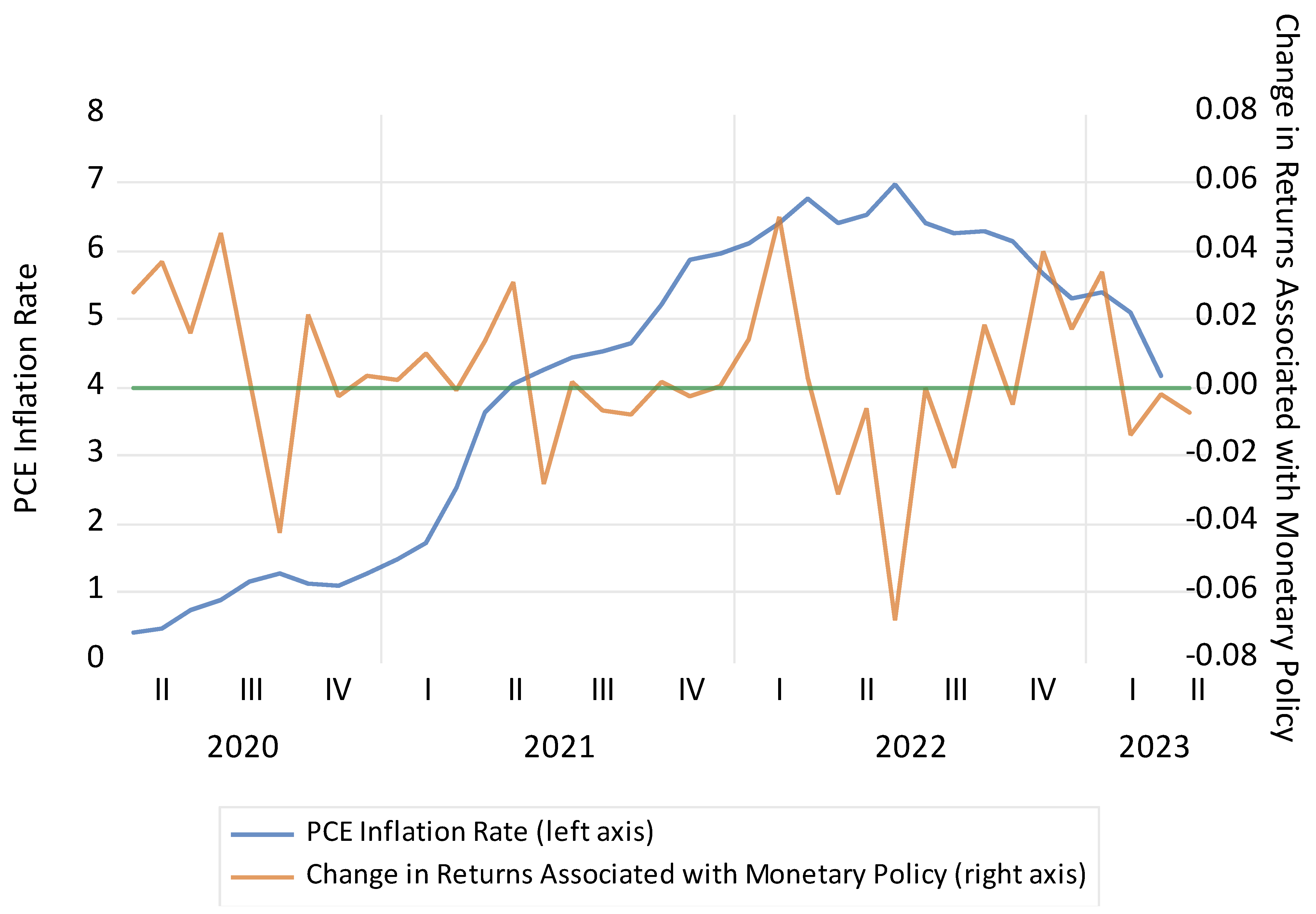
To understand how investors interpreted monetary policy actions after the pandemic, Figure 1 plots the results from regressing returns on the 53 assets on their BRW monetary policy betas over the April 2020 to April 2023 period. To facilitate interpretation, the regression coefficient is multiplied by the monetary policy beta for the market portfolio.7 Since the monetary policy beta for the market portfolio is negative, the product of the market portfolio monetary policy beta and the regression coefficient is positive when investors expect Fed policy to become easier and negative when they foresee tighter policy. The coefficients in Figure 1 show how investors’ responses to monetary policy news affected the return on the market portfolio. Figure 1 also plots the year-on-year increase in the Fed’s preferred inflation measure, the PCE price index.

The figure shows that investors in April, May, June, and July 2020 expected the path of monetary policy to become looser. Easier monetary policy seemed appropriate at this time as the economy faced headwinds from a once-in-a-lifetime pandemic, as nonfarm employment between March and July 2020 fell by 52 standard deviations, and as the PCE inflation rate was below 1%.

The figure also shows that in 2021, the PCE inflation rate rose from 1.5% to 6.1%, reaching its highest level in 40 years. As inflation soared in 2021, however, investors only foresaw tighter monetary policy in one month. They even priced in easier monetary policy in April and May 2021. While Adams et al. (2023) reported that the Fed’s communication pivot towards a tightening cycle worsened sentiment in September 2021, there is no evidence in Figure 1 that investors bid down stock prices in September in response to this.

As inflation increased by another 200 basis points in 2022, the Fed reacted violently by increasing its federal funds rate target by 500 basis points. Figure 1 shows that investors priced in contractionary shifts in the course of policy over several months in 2022. One thing that is striking in Figure 1 is the magnitude of the stock market response. For instance, in June 2022, anticipations of contractionary monetary policy pushed down returns on the market portfolio by 6.7%. For aluminum, the asset most exposed to monetary policy in Table 3, contractionary monetary policy pushed down returns in June 2022 by more than 22.3%.

A second thing that is striking in Figure 1 is how investors’ perceptions beginning in 2022 changed from month to month. Over the next 16 months, their expectations frequently changed from anticipating easier policy to anticipating tighter policy to anticipating easier policy again. The beta values in Table 3 indicate that monetary policy exerts important effects on many stocks, and during the drastic tightening in 2022, investors focused on how these stocks would be affected by changes in the future course of monetary policy. Stock prices rose and fell several times in response to changing monetary policy perceptions.

There are some puzzling data points in Figure 1. For instance, in February 2023, investors expected the path of monetary policy to become tighter even as the PCE inflation rate was falling rapidly. Investors also possessed additional information relevant to inflation and monetary policy. For instance, surges in COVID-19 infections disrupted supply chains, reduced labor supply, and stoked inflation from the supply side. To shed light on these issues, Figure 2 plots the CPI inflation rate, the core CPI inflation rate, and the number of new COVID-19 infections.

Figure 2 helps explain why investors priced in more contractionary monetary policy in February 2023, even as the PCE inflation rate was tumbling. The CPI inflation rate was also falling, but the core CPI rate was not. Thus, the Fed needed to continue fighting inflation even though the headline inflation rate was falling. Also, investors began pricing in tighter monetary policy in 2022 after the number of COVID-19 cases spiked. The surge in cases increased expected inflation through the supply side by disrupting supply chains and reducing labor supply.

Figure 3 examines the stock market responses during the volatile period from April to August 2022 using daily data. It plots changes in returns on the market portfolio associated with monetary policy for all of the business days between 1 April 2022 and 31 August 2022 when there was a statistically significant relationship at least at the 10% level between the returns on the 53 assets and their BRW monetary policy betas. The figure indicates that, of the 109 business days over this period, there was a systematic reaction to monetary policy news on 41 days. Thus, investors priced in changes in the future path of monetary policy on almost 40% of the days.

Many of the dates plotted in Figure 3 correspond to dates when there was important news related to monetary policy. For instance, the 0.7% drop in Figure 3 on April 6 occurred on the day when the minutes from the previous FOMC meeting indicated that many officials had wanted a larger funds rate increase in March 2022 (Megaw et al. 2022). The 1.0% drop on May 12 occurred when Fed Chair Powell warned that taming inflation would cause pain (Smith 2022b). The 1.5% drop on June 23 happened as Fed officials voiced support for a 0.75 percentage point rise in the federal funds rate target at the next policy meeting (Smith 2022a). The 1.2% drop on July 14 came as news of higher than expected inflation drove expectations of larger increases in the federal funds rate target (Johnson 2022). The 0.5% decrease on August 29 occurred after several central bankers warned of higher rates (Lockett et al. 2022).

Figure 3 indicates that news about monetary policy contributed to large swings in stock returns. As the Fed in 2022 began what Eggertsson and Kohn (2023) called an unprecedented increase in the federal funds rate, investors drove stock prices up and down in response to changing perceptions about the future path of monetary policy. Arteta et al. (2022) found that much of the Fed’s impact on financial markets in 2022 occurred because investors kept updating their beliefs about the Fed’s preferences towards inflation. As the Fed pursued drastic tightening, it sewed confusion and multiplied volatility in the U.S. stock market, one of the world’s most important financial markets.

Figure 1 indicates that investors priced in easier monetary policy in January 2023. At this time, though, the measure of monetary policy uncertainty constructed using the methods of Baker et al. (2016) reached the fifth highest level over the 460 months for which data are available.8 Complex uncertainty concerning the future path of monetary policy thus continued into 2023. By increasing uncertainty and spawning volatility, the Fed made firms more hesitant to invest (see, e.g., Bloom et al. 2007).

4. Conclusions

The Federal Reserve was slow to recognize that inflation after the pandemic would persist. It did not tighten policy until 2022, after the PCE inflation rate reached its highest level in more than 40 years. It then undertook an unprecedented tightening, raising the federal funds rate by 500 basis points in 15 months. These actions multiplied stock market volatility. They also contributed to 26% losses in both long-term corporate and Treasury bonds in 2022. This is by far the worst bond market performance over the 97 years that Kroll (2023) provides data. Rajan (2023) noted that the Fed’s highly expansionary policies before 2022 generated financial instability by pushing investors into riskier, higher-yielding assets that performed badly when the Fed tightened.

What can central bankers learn from this experience? Huw Pill, the chief economist at the Bank of England, noted that the economic models they used to forecast inflation after the pandemic were estimated over periods when shocks were less extreme (Giles 2023). Regression techniques are only valid locally and are unreliable when extrapolated outside of the range of observed data.9 Policymakers’ perspectives were also formed during periods when inflation was quiescent, and this contributed to misinterpreting the inflationary shocks that began in 2021 as transitory.

Faced with extreme or unusual events, policymakers should learn from historical episodes, dialogue with others whose worldviews differ from theirs, and communicate well. History does not repeat itself, but it rhymes. Studying similar events in the past can shed light on how shocks will impact inflation and other key variables in the present.

Listening to people with different perspectives can also be beneficial. Granovetter (1973) showed that people who work closely together tend to think alike. When the economy faces unusual shocks, it is salutary for FOMC members to exchange ideas with others with whom they share only “weak ties”. This can expose policymakers to new ideas, enable them to reevaluate their own implicit models, and help them understand why their forecasts might prove wrong.

Adams et al. (2023) found that Fed communication pivoted towards a tightening cycle in 2021. However, the results reported here indicate that markets only began pricing in monetary tightening in 2022. Eggertsson and Kohn (2023) observed that many were uncertain of the Fed’s intentions. Dietrich et al. (2022) found that better communication by the central bank with the public could have mitigated uncertainty. Arteta et al. (2022) reported that changing perceptions about the Fed’s preferences towards inflation explained much of the movement in asset prices in 2022 and concluded that proper communication that clarified the Fed’s reaction function could have reduced adverse spillovers. Improved communication could thus have helped to attenuate the wild swings in stock prices that arose because of uncertainty about monetary policy.

The economy will face challenging shocks going forward. It may respond differently to these than it has to shocks in the past. Central bankers need to be nimble, pragmatic, and skillful at updating their beliefs about how the world works.

References

- Adams, Travis, Andrea Ajello, Diego Silva, and Francisco Vazquez-Grande. 2023. More than Words: Twitter Chatter and Financial Market Sentiment. Working Paper No. 2023-034, Finance and Economics Discussion Series. Washington, DC: Board of Governors of the Federal Reserve System. [Google Scholar]
- Arteta, Carlos, Steven Kamin, and Franz Ulrich Ruch. 2022. How Do Rising U.S. Interest Rates Affect Emerging and Developing Economies? It Depends. Policy Research Working Paper 10258. Washington, DC: World Bank. [Google Scholar]
- Baker, Scott, Nicholas Bloom, and Steven Davis. 2016. Measuring Economic Policy Uncertainty. Quarterly Journal of Economics 131: 1593–636. [Google Scholar] [CrossRef]
- Bauer, Michael, and Eric Swanson. 2022. A Reassessment of Monetary Policy Surprises and High-Frequency Identification. In NBER Macroeconomics Annual 2022. Edited by Martin Eichenbaum, Erik Hurst and Valerie Ramey. Chicago: University of Chicago Press, vol. 37. [Google Scholar]
- Bekaert, Geert, and Xiaozheng Wang. 2010. Inflation Risk and the Inflation Risk Premium. Economic Policy 25: 755–806. [Google Scholar] [CrossRef]
- Bernanke, Ben, and Kenneth Kuttner. 2005. What Explains the Stock Market’s Reaction to Federal Reserve Policy? Journal of Finance 60: 1221–57. [Google Scholar] [CrossRef]
- Bernanke, Ben, and Olivier Blanchard. 2023. What Caused the U.S. Pandemic-Era Inflation? Presentation at Hutchins Center, Brookings Institution, 23 May. Available online: https://www.brookings.edu/wp-content/uploads/2023/04/Bernanke-Blanchard-conference-draft_5.23.23.pdf (accessed on 10 July 2023).
- Bloom, Nicholas, Steven Bond, and John Van Reenen. 2007. Uncertainty and Investment Dynamics. The Review of Economic Studies 74: 391–415. [Google Scholar] [CrossRef]
- Boudoukh, Jacob, Matthew Richardson, and Richard Whitelaw. 1994. Industry Returns and the Fisher Effect. Journal of Finance 44: 1595–615. [Google Scholar] [CrossRef]
- Bu, Chunya, John Rogers, and Wenbin Wu. 2021. A Unified Measure of Fed Monetary Policy Shocks. Journal of Monetary Economics 118: 331–49. [Google Scholar] [CrossRef]
- Campbell, John Young, and John Ammer. 1993. What Moves the Stock and Bond Markets? A Variance Decomposition for Long-term Asset Returns. Journal of Finance 48: 3–37. [Google Scholar]
- Campbell, John Young, and Tuomo Vuolteenaho. 2004. Bad Beta, Good Beta. American Economic Review 94: 1249–75. [Google Scholar] [CrossRef]
- Chen, Nai-Fu, Richard Roll, and Stephen Ross. 1986. Economic Forces and the Stock Market. Journal of Business 59: 383–403. [Google Scholar] [CrossRef]
- Chibane, Messaoud, and Ano Kuhanathan. 2023. Is The Fed Failing To Re-Anchor Expectations? An Analysis of Jumps in Inflation Swaps. Finance Research Letters. forthcoming. [Google Scholar]
- Cieslak, Anna, and Carolin Pflueger. 2023. Inflation and Asset Returns. Working Paper No. 30982. Cambridge: National Bureau of Economic Research. [Google Scholar]
- CRR. 1996. 18 Juillet 1986, no. 50265, M. D. France: Commission des Recours des Réfugiés (CRR), July 18. [Google Scholar]
- Dietrich, Alexander, Keith Kuester, Gernot Müller, and Raphael Schoenle. 2022. News and Uncertainty about COVID-19: Survey Evidence and Short-run Economic Impact. Journal of Monetary Economics 129: S35–S51. [Google Scholar] [CrossRef] [PubMed]
- Eggertsson, Gauti, and Don Kohn. 2023. The Inflation Surge of the 2020s: The Role of Monetary Policy. Presentation at Hutchins Center, Brookings Institution, 23 May. Available online: https://www.brookings.edu/wp-content/uploads/2023/04/Eggertsson-Kohn-conference-draft_5.23.23.pdf (accessed on 10 July 2023).
- Fama, Eugene, and James MacBeth. 1973. Risk, Return, and Equilibrium: Empirical Tests. Journal of Political Economy 81: 607–36. [Google Scholar] [CrossRef]
- Frankel, Jeffrey. 2008. The Effect of Monetary Policy on Real Commodity Prices. In Asset Prices and Monetary Policy. Edited by John Young Campbell. Chicago: University of Chicago Press, pp. 291–333. [Google Scholar]
- Furman, Jason. 2023. Inflation: A Series of Unfortunate Events vs. Original Sin. Presentation at Hutchins Center, Brookings Institution, 23 May. Available online: https://www.brookings.edu/wp-content/uploads/2023/04/20230523-Hutchins-Inflation-Comment-v2.pdf (accessed on 10 July 2023).
- Gagliardone, Luca, and Mark Gertler. 2023. Oil Prices, Monetary Policy and Inflation Surges. Working Paper No. 31263. Cambridge: National Bureau of Economic Research. [Google Scholar]
- Gallant, Ronald. 1975. Nonlinear Regression. The American Statistician 29: 73–81. [Google Scholar]
- Giles, Chris. 2023. Bank of England Admits ‘Very Big Lessons to Learn’ over Failure to Forecast Rise in Inflation. Financial Times, May 24. [Google Scholar]
- Granovetter, Mark. 1973. The Strength of Weak Ties. American Journal of Sociology 78: 1360–80. [Google Scholar] [CrossRef]
- Hanson, Samuel G., and Jeremy C. Stein. 2015. Monetary Policy and Long-Term Real Rates. Journal of Financial Economics 115: 429–48. [Google Scholar] [CrossRef]
- Hornstein, Andreas. 2022. Recession Predictors: An Evaluation. Economic Brief No. 22–30. Richmond: Federal Reserve Bank of Richmond. [Google Scholar]
- Johnson, Ian. 2022. US Government Debt Under Pressure as Markets Price in Larger Rate Rises. Financial Times, July 14. [Google Scholar]
- Kashyap, Anil, and Jeremy Stein. 2023. Monetary Policy When the Central Bank Shapes Financial-Market Sentiment. Journal of Economic Perspectives 37: 53–76. [Google Scholar] [CrossRef]
- Kroll. 2023. 2023 SBBI Yearbook. New York: Kroll. [Google Scholar]
- Lockett, Hudson, Philip Stafford, and Nicholas Megaw. 2022. Global Equities Drop on Warning over Sustained Rate Rises. Financial Times, August 30. [Google Scholar]
- McElroy, Marjorie, and Edwin Burmeister. 1988. Arbitrage Pricing Theory as a Restricted Nonlinear Multivariate Regression Model: Iterated Nonlinear Seemingly Unrelated Regression Estimates. Journal of Business & Economic Statistics 6: 29–42. [Google Scholar]
- Megaw, Nicholas, Naomi Rovnik, and William Langley. 2022. US Stocks End Lower after Fed Minutes Point to Tighter Monetary Policy. Financial Times, April 7. [Google Scholar]
- Milstein, Eric, and David Wessel. 2021. What Did the Fed Do in Response to the COVID-19 Crisis? Brookings Weblog. December 17. Available online: https://www.brookings.edu/research/fed-response-to-covid19/ (accessed on 10 July 2023).
- Rajan, Raghuram. 2023. Not Buying Central Banks’ Favorite Excuse. Project Syndicate Weblog, May 26. [Google Scholar]
- Ross, Stephen. 2001. Finance. In The New Palgrave Dictionary of Money and Finance. Edited by Peter Newman, Murray Milgate and John Eatwell. London: Macmillan Press, pp. 1–34. [Google Scholar]
- Smith, Colby. 2022a. Support Grows Among Fed Officials for Further 0.75 Percentage Point Rate Rise. Financial Times, June 24. [Google Scholar]
- Smith, Colby. 2022b. Powell Warns that Taming Inflation Will Cause Some Pain. Financial Times, May 13. [Google Scholar]
- Thorbecke, Willem. 2018. The Effect of the Fed’s Large-scale Asset Purchases on Inflation Expectations. Southern Economic Journal 85: 407–23. [Google Scholar] [CrossRef]
Figure 1.
The personal consumption expenditures (PCE) inflation rate and the monthly change in returns on the market portfolio associated with exposure to monetary policy. Note: The figure presents the personal consumption expenditures (PCE) inflation rate and the change in returns on the market portfolio associated with monetary policy. To calculate the change in returns associated with monetary policy, assets’ monetary policy betas are estimated. The betas are obtained from an iterated nonlinear seemingly unrelated regression of returns on 53 assets (minus the return on one-month Treasury bills) on the Bu et al. (2021) (BRW) measure of Fed policy surprises, the difference in returns between 20-year and one-month Treasury securities, the monthly growth rate in industrial production, unexpected inflation, and the change in expected inflation. The BRW measure is constructed so that an increase represents a contractionary monetary policy surprise. If investors believe that monetary policy will tighten, this will drive up the prices of assets that benefit from contractionary monetary policy (those with larger betas to the BRW variable) and drive down the process of assets that are harmed by contractionary monetary policy (those with smaller betas to the BRW variable). There should thus be a positive relationship between asset returns and assets’ BRW betas on months when investors foresee monetary policy tightening. For each month between April 2020 and April 2023, returns on the 53 assets are thus regressed on the assets’ monetary policy betas. To facilitate interpretation, the resulting regression coefficient is multiplied by the beta coefficient on the market portfolio obtained from regressing the return on the S&P 500 on the BRW measure of monetary policy, unexpected inflation, the horizon premium, industrial production growth, and the change in expected inflation over the January 1994 to December 2019 period. The change in returns associated with monetary policy in the figure thus represents the change in returns for the market portfolio. Since the market monetary policy beta is negative, positive values in Figure 1 indicate that investors expect easier policy and negative values indicate that they foresee tighter policy.
Figure 2.
The consumer price index, the core consumer price index, and the number of new COVID-19 Cases in the U.S. Source: Federal Reserve Bank of St. Louis FRED database and Our World in Data (https://ourworldindata.org/covid-cases accessed on 5 September 2023).
Figure 3.
The daily change in returns on the market portfolio associated with exposure to monetary policy between 1 April and 31 August 2022. Note: The figure presents the daily change in returns associated with monetary policy. To calculate the change in returns associated with monetary policy, assets’ monetary policy betas are estimated. The betas are obtained from an iterated nonlinear seemingly unrelated regression of returns on 53 assets (minus the return on one-month Treasury bills) on the Bu et al. (2021) (BRW) measure of Fed policy surprises, the difference in returns between 20-year and one-month Treasury securities, the monthly growth rate in industrial production, unexpected inflation, and the change in expected inflation. The BRW measure is constructed so that an increase represents a contractionary monetary policy surprise. If investors believe that monetary policy will tighten, this will drive up the prices of assets that benefit from contractionary monetary policy (those with larger betas to the BRW variable) and drive down the process of assets that are harmed by contractionary monetary policy (those with smaller betas to the BRW variable). There should thus be a positive relationship between asset returns and assets’ BRW betas on days when investors foresee tighter monetary policy. For each business day between 1 April 2022 and 31 August 2022, returns on the 53 assets are thus regressed on the assets’ monetary policy betas. To facilitate interpretation, the regression coefficient is multiplied by the monetary policy beta for the market portfolio obtained from regressing the return on the S&P 500 on the BRW measure of monetary policy, unexpected inflation, the horizon premium, industrial production growth, and the change in expected inflation over the January 1994 to December 2019 period. The change in returns associated with monetary policy in the figure thus represents the change in returns for the market portfolio. Since the market BRW beta coefficient is negative, positive values in Figure 3 indicate that investors expect easier policy and negative values indicate that they foresee tighter policy. The figure only reports days when there is a statistically significant relationship (at least the 10 percent level) between returns on the 53 assets and the assets’ monetary policy betas.