On the Impact of Policy Uncertainty on Oil Prices: An Asymmetry Analysis

Abstract

Previous research has assessed the impact of policy uncertainty on a few macro variables. In this paper, we consider its impact on oil prices. Oil prices are usually determined in global markets by the law of demand and supply. Our concern in this paper is to determine which country’s policy uncertainty measure has an impact on oil prices. Using both the linear and the nonlinear Autoregressive Distributed Lag (ARDL) methods, we find that while policy uncertainty measures of Canada, China, Europe, Japan, Russia, South Korea, and the U.S. have short-run effects, short-run effects last into the long-run asymmetric effects only in the case of China. This may reflect the importance and recent surge in China’s engagement in world trade.

1. Introduction

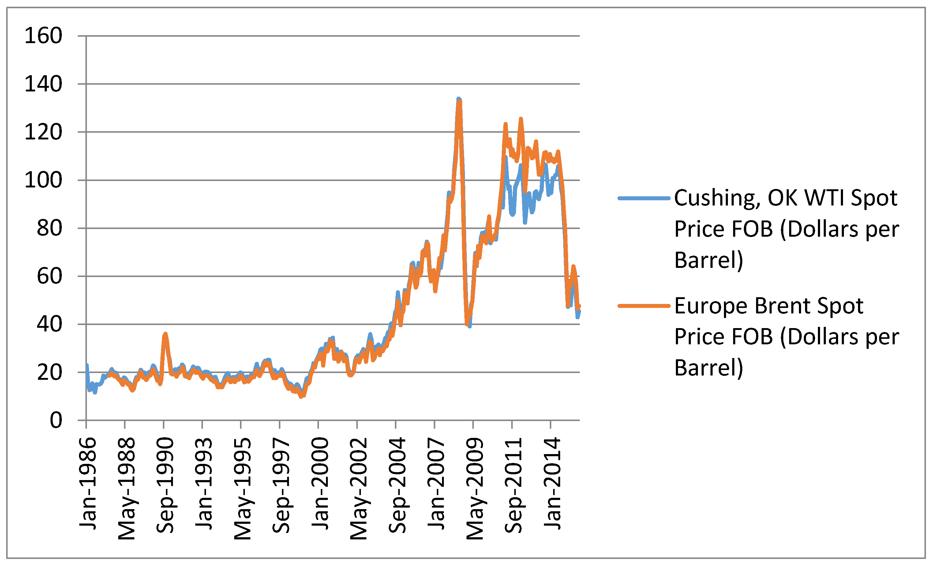
In response to imported inflation from the West, members of the OPEC decided to raise the price of oil from $2.60 to $12 per barrel in 1973, introducing an uncertain environment to future prices. Due to Iranian revolution in 1979 and unrest in Middle East, the prices rose again to $46 and, ever since, oil prices have fluctuated and contributed to uncertain oil prices. Figure 1 shows movement of two measures of oil prices over time.

A large literature in economics predicts that oil price uncertainty or volatility could have adverse effects on many macro variables such as investment, consumption, real GDP, etc. While Bernanke (1983), Brennan and Schwartz (1985), Majd and Pindyck (1987), Brennan (1990), Triantis and Hodder (1990), and Elder and Serletis (2010) emphasize its impact on investment, Kim and Loungani (1992), Hooker (1996), and Finn (2000) emphasize its impact on economic activity. Furthermore, impact of oil price uncertainty on consumption and investment is considered by Edelstein and Kilian (2009) and on economic activity and stock returns by Kang et al. (2017a).

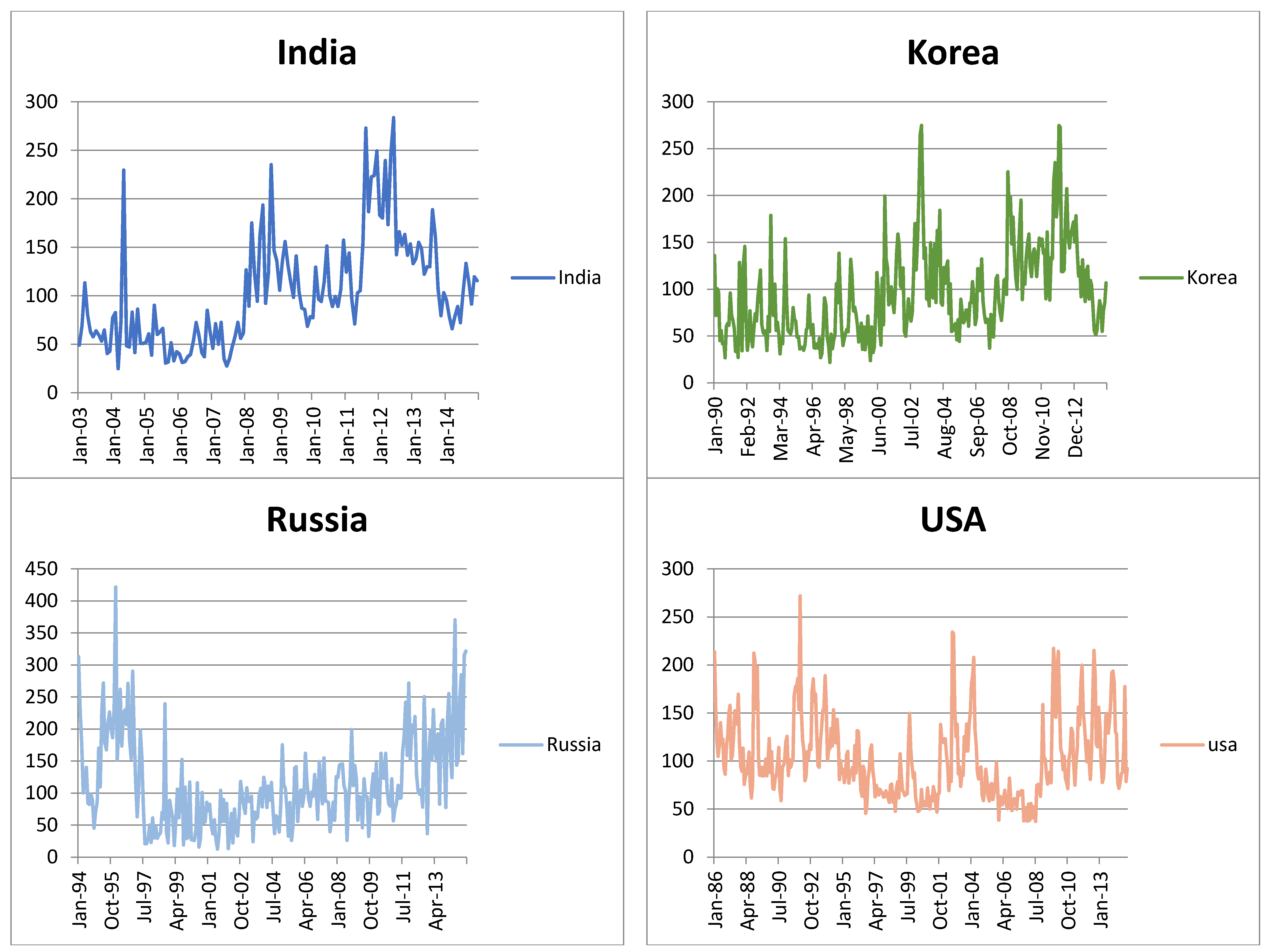
In addition to global events such as the U.S. invasion of Iraq or Iran-Iraq war in the 1980s that affected oil prices, any uncertain action in the major oil consuming countries could also have an implication for oil prices. Uncertainty in a given country could originate from many factors such as government’s decision to settle its budget, terrorist activity in a given country, change in political system, changes in rules and regulations governing taxes and investment, etc. Although it seems difficult to construct a measure of uncertainty that accounts for all of these events or activities that take place within an individual country, the Policy Uncertainty Group constructs and publishes such measure on its website.1 The measure is known as the measure of policy uncertainty and to construct it, our group follows Baker et al. (2016) and searches for such terms as “policy”, “tax”, “spending”, “regulation”, “central bank”, “budget”, “uncertain”, “uncertainty”, “deficit”, etc., from as many newspapers as possible in each country, and then a normalized index of the volume of news articles is constructed. While one news outlet may discuss a specific aspect of uncertainty by one policy, another outlet may discuss another aspect. The higher such discussions are associated with different uncertainty factors, the higher the importance of the news and the larger the “policy uncertainty” measure. In order to gain some insight into performance of this uncertainty measure in each country in this study, we plot them in Figure 22.

A few studies have emphasized the importance of policy uncertainty in predicting future oil prices. Bekiros et al. (2015) use a few different methods and concludes that the time-varying VAR model outperforms alternative models. Kang et al. (2017b), on the other hand, use the policy uncertainty measure to show that when it rises, it damages the stock returns of oil and gas corporations. Finally, rather than assessing the impact of policy uncertainty on oil prices, Demir and Gozgor (2016) investigate the effects of policy uncertainty on oil-related consumption such as vehicle miles traveled in the U.S. They find that an increase in economic policy uncertainty leads to a decrease in vehicle miles traveled.

Our goal in this paper is to determine which country’s policy uncertainty affects oil prices in global markets. Clearly, an uncertain action in a large oil consuming country is expected to have relatively a greater number of and more significant effects compared to a small country. In addition to assessing the impact of each country’s policy uncertainty on oil prices, we would like to determine if the effects are asymmetric. For that purpose, we introduce the methods in Section 2 and present our findings in Section 3. A summary is provided in Section 4 and data definition and sources are provided in an Appendix A.

2. The Models and Methods

Let OP denote oil prices and PU denote policy uncertainty measure. We begin with the following bivariate model:

$$LnOPt=\alpha +\beta LnP{U}_t,+{\epsilon }_t$$

(1)

Specification (1) is a long-run specification which could be estimated by the Ordinary Least Squares (OLS) to determine if an increase in policy uncertainty has positive impact on oil prices. Thus, an estimate of β reflects the long-run effects of PU on OP. In order to assess the short-run effects, we follow Pesaran et al. (2001) and convert (1) to an error-correction specification as in (2):

$$\Delta LnO{P}_t=a+{\displaystyle \sum _{i=1}^{n1}{b}_{i}LnO{P}_{t-i}}+{\displaystyle \sum _{i=0}^{n2}{c}_{i}Ln\Delta P{U}_{t-i}}+{\lambda }_{0}LnO{P}_{t-1}+{\lambda }_{1}LnP{U}_{t-1}+{\mu }_t$$

(2)

The model outlined by (2) is an error-correction model that could be estimated using a set lag selection criterion. Once estimated, short-run effects of policy uncertainty are inferred by the estimates of c_i’s and its long-run effects by the estimate of λ₁ normalized on λ₀ as ${\widehat{\lambda }}_1/-{\widehat{\lambda }}_0$. However, in order to avoid spurious estimates, cointegration must be established. Pesaran et al. (2001) propose two tests. The first is the F test applied to joint significance of lagged level variables with new critical values that they tabulate. The second test is a t-test. Under this second test, normalized long-run estimates and long-run model (1) are used to generate the error terms, denoted by ECM. Then, after replacing a linear combination of lagged level variables by ECM_t-1, the new specification is estimated at the same optimum lags. Cointegration is established if ECM_t-1 carries a significantly negative coefficient. Since the t-test is used to judge significance of this estimate, the test is also known as the t-test. Pesaran et al. (2001) provide new critical values for both tests that account for integrating properties of variable as long as they are integrated of order zero, I(0), or one, I(1). Since most macro variables are either I(0) or I(1), there is no need for pre-unit root testing.

One main assumption in (1) is that oil prices respond to changes in policy uncertainty in an asymmetric manner. However, this need not be the case. Increased policy uncertainty could affect oil prices at different rates compared to decreased uncertainty. Suppose an x% increase in uncertainty measure raises oil prices by y%. However, when uncertainty declines by x%, since markets become more optimistic about the changed situation in a given country, oil prices may decline by less than y%, hence an asymmetric effect. Alternatively, downward price rigidity in oil markets mostly due to production cut by OPEC could also be a source of asymmetric effects. To assess the asymmetric effects of policy uncertainty on oil prices, we follow Shin et al. (2014) and form ΔLnPU which includes positive changes reflecting an increase in the policy uncertainty measure and negative changes reflecting declines. We then construct two new times series variables as outlined by specification (3):

$$PO{S}_t^{}={\displaystyle \sum _{j=1}^t\max (\Delta LnP{U}_j},0),NE{G}_t^{}={\displaystyle \sum _{j=1}^t\min (\Delta LnP{U}_j,0)}$$

(3)

where POS which is the partial sum of positive changes reflects only increase in policy uncertainty measure and NEG which is the partial sum of negative changes, reflects only decrease in policy uncertainty. We then shift back to Equation (2) and replace LnPU by the two partial sum variables to arrive at specification (4):

$$\begin{array}{ll}\Delta LnO{P}_t=a\prime & +{\displaystyle \sum _{i=1}^{n1}b{\prime }_{i}LnO{P}_{t-i}}+{\displaystyle \sum _{i=0}^{n2}c{\prime }_i\Delta PO{S}_{t-i}}+{\displaystyle \sum _{i=0}^{n3}d{\prime }_i}\Delta NE{G}_{t-i}+{\rho }_{0}LnO{P}_{t-1}\\ & +{\rho }_{1}PO{S}_{t-1}+{\rho }_{2}NE{G}_{t-1}+{\mu }_t\end{array}$$

(4)

Specification (4) is another error-correction model which could be used to assess the asymmetric effects of policy uncertainty on oil prices. Such models are labeled nonlinear ARDL models mostly due to method of constructing the partial sum variables. However, models like (2) are called linear ARDL model.

Shin et al. (2014) demonstrate that Pesaran et al.’s (2001) approach of estimating (2) and applying the F and t tests to establish cointegration are equally applicable to (4). They even recommend that in applying the F test, the two partial sum variables should be treated as a single variable so that the critical value of the F test stays at conservatively high level. Once (4) is estimated using a set lag selection criterion, a few asymmetry assumptions could be tested. First, if estimates of c′ and d′ are different at the same lag, short-run asymmetric effects will be established. Second, if the null of ${\displaystyle \sum {\widehat{c}}_i^{\prime }={\displaystyle \sum {\widehat{d}}_i^{\prime }}}$ is rejected by the Wald test, that will be an indication of short-run cumulative or impact asymmetry. Third, if n2 ≠ n3, i.e., the two partial sum variables take different lag order, and adjustment asymmetry will be supported. Finally, if the null hypothesis of $\raisebox{1ex}{${\widehat{\rho }}_1$}\!\left/ \!\raisebox{-1ex}{$-{\widehat{\rho }}_0$}\right.=\raisebox{1ex}{${\widehat{\rho }}_2$}\!\left/ \!\raisebox{-1ex}{$-{\widehat{\rho }}_0$}\right.$, i.e., equality of normalized long-run coefficients attached to partial sum variables is rejected by the Wald test, long-run asymmetric effects of policy uncertainty on oil prices will be established.3

3. Empirical Results

In this section we estimate both the linear model (2) and the nonlinear model (4) using monthly data from each of the nine countries in our sample. The list of the countries, study period for each, sources of the data, and definition of variables are provided in the Appendix A. Since there are different critical values for different statistics, we have reported them in the notes to

Table 1. Full-Information Estimates of Both Linear ARDL (L-ARDL) and Nonlinear ARDL (NL-ARDL) Models. Wald statics are both distributed as χ² with one degree of freedom.

	Canada		China		Dutch
	L-ARDL	NL-ARDL	L-ARDL	NL-ARDL	L-ARDL	NL-ARDL
Panel A: Short–Run Estimates
ΔlnOPt-1	0.24 (4.45) **	0.28 (5.24) **	0.25 (3.82) **	0.24 (3.68) **	0.28 (3.22) **	0.29 (3.34) **
ΔlnOPt-2				0.13 (1.98) **	0.23 (2.57) **	0.24 (2.66) **
ΔlnOPt-3
ΔlnOPt-4
ΔlnOPt-5
ΔlnOPt-6
ΔlnPUt	−0.04 (2.61) **		−0.01 (0.93)		−0.04 (1.57)
ΔlnPUt-1	−0.06 (3.73) **
ΔlnPUt-2	−0.03 (2.38) **
ΔlnPUt-3	−0.02 (1.79) *
ΔlnPUt-4
ΔlnPUt-5
ΔlnPUt-6
ΔlnPUt-7
ΔPOSt		−0.05 (2.52) **		−0.07 (1.36)		−0.05 (1.23)
ΔPOSt-1				−0.09 (2.57) **
ΔPOSt-2
ΔPOSt-3
ΔPOSt-4
ΔPOSt-5
ΔPOSt-6
ΔPOSt-7
ΔNEGt		−0.07 (1.26)		0.02 (0.57)		−0.07 (1.43)
ΔNEGt-1		−0.14 (2.43) **		0.09 (1.79) *
ΔNEGt-2
ΔNEGt-3
ΔNEGt-4
ΔNEGt-5
ΔNEGt-6
ΔNEGt-7
Panel B: Long-Run Estimates
ln PU	−2.03 (0.56)		−0.89 (0.62)		0.15 (0.57)
POS		−1.87 (1.62)		−0.95 (2.05) **		−0.44 (1.21)
NEG		−2.01 (1.72) *		−1.05 (2.23) **		−0.54 (1.44)
Constant	13.47 (0.78)	2.06 (5.11) **	8.19 (1.20)	2.62 (10.57) **	3.67 (3.17)	3.83 (24.41) **
Panel C: Diagnostic Statistics
F	1.33	3.66	1.80	5.81 *	4.89 *	4.66
ECMt-1	−0.01 (0.82)	−0.03 (2.33)	−0.01 (1.15)	−0.08 (3.57) **	−0.07 (3.07) *	−0.12 (3.64) **
LM	15.39	15.12	11.94	10.83	15.35	14.63
RESET	5.91 **	1.45	5.31 **	3.69 *	8.13 **	8.44 **
Adjusted R2	0.11	0.08	0.06	0.07	0.14	0.14
CS (CS2)	S (S)	S (S)	S (S)	S (S)	S (US)	S (US)
WALD–S		0.81		4.43 **		0.07
WALD–L		17.47 **		72.42 **		5.37 **
	Europe		India		Japan
	L-ARDL	NL-ARDL	L-ARDL	NL-ARDL	L-ARDL	NL-ARDL
Panel A: Short–Run Estimates
ΔlnOPt-1	0.28 (5.20) **	0.29 (5.43) **	0.28 (3.22) **	0.30 (3.59) **	0.29 (5.18) **	0.29 (5.37) **
ΔlnOPt-2			0.22 (2.39) **	0.26 (2.98) **
ΔlnOPt-3			−0.07 (0.78)
ΔlnOPt-4			−0.01 (0.15)
ΔlnOPt-5			0.08 (0.91)
ΔlnOPt-6			−0.23 (2.66) **
ΔlnPUt	−0.03 (1.51)		0.002 (0.14)		−0.05 (3.06) **
Δln PUt-1	−0.05 (2.83) **				−003 (1.84) *
ΔlnPUt-2	−0.06 (3.11) **
ΔlnPUt-3	−0.04 (2.38) **
ΔlnPUt-4
ΔlnPUt-5
ΔlnPUt-6
ΔlnPUt-7
ΔPOSt		−0.03 (0.54)		−0.002 (0.07)		−0.05 (0.78)
ΔPOSt-1		−0.14 (2.43) **				−0.19 (2.75)
ΔPOSt-2		−0.04 (0.74)				−0.02 (0.27)
ΔPOSt-3		0.06 (1.10)				−0.06 (0.94)
ΔPOSt-4		0.02 (0.49)				−0.09 (1.36)
ΔPOSt-5		0.12 (2.20) **				−0.18 (2.86) **
ΔPOSt-6
ΔPOSt-7
ΔNEGt		0.09 (2.49) **		−0.01 (0.34)		−0.19 (2.89) **
ΔNEGt-1
ΔNEGt-2
ΔNEGt-3
ΔNEGt-4
Panel B: Long-Run Estimates
ln PU	−1.00 (0.34)		0.04 (0.15)		−1.92 (0.82)
POS		−2.27 (1.86) *		−0.02 (0.07)		−0.86 (0.86)
NEG		−2.46 (1.96) **		−0.10 (0.34)		−0.97 (0.97)
Constant	8.63 (0.62)	2.68 (5.39) **	4.15 (3.08) **	3.84 (24.77) **	12.63 (1.16)	3.65 (5.40) **
Panel C: Diagnostic Statistics
F	1.03	3.68	3.08	5.49 *	1.69	2.74
ECMt-1	−0.01 (0.90)	−0.03 (2.74)	−0.05 (2.02)	−0.12 (3.60) **	−0.01 (1.37)	−0.04 (2.74)
LM	11.46	13.66	8.04	15.52	9.49	8.92
RESET	3.89 *	4.06 **	3.59 *	7.02 **	1.07	0.48
Adjusted R2	0.12	0.12	0.15	0.09	0.11	0.13
CS (CS2)	S (S)	S (S)	S (S)	S (S)	S (S)	S (S)
WALD–S		0.10		0.49		4.36 **
WALD–L		21.88 **		6.81 **		24.91 **
	Russia		South Korea		United States
	L-ARDL	NL-ARDL	L-ARDL	NL-ARDL	L-ARDL	NL-ARDL
Panel A: Short–Run Estimates
ΔlnOPt-1	0.26 (4.11) **	0.24 (3.77) **	0.26 (4.55) **	0.26 (4.64) **	0.28 (5.60) **	0.31 (5.86) **
ΔlnOPt-2		0.15 (2.32) **
ΔlnOPt-3
ΔlnOPt-4
ΔlnOPt-5
ΔlnOPt-6
ΔlnPUt	−0.01 (0.71)		−0.02 (1.45)		−0.34 (0.01)
ΔlnPUt-1	−0.02 (1.52)		−0.08 (4.79) **		−0.07 (2.43) **
ΔlnPUt-2	−0.02 (2.29) **		−0.05 (2.89) **		−0.04 (1.53)
ΔlnPUt-3			−0.06 (4.07) **
ΔlnPUt-4			−0.04 (2.36) **
ΔlnPUt-5			−0.03 (2.25) **
ΔlnPUt-6			−0.04 (2.65) **
ΔlnPUt-7			−0.02 (1.66) *
ΔPOSt		−0.005 (0.15)		0.03 (0.55)		−0.01 (0.06)
ΔPOSt-1		−0.07 (2.16) **		−0.05 (1.11)		−0.28 (2.83) **
ΔPOSt-2		−0.12 (3.48) **		−0.05 (1.05)		−0.14 (1.47)
ΔPOSt-3		−0.06 (1.72) *		−0.15 (3.36) **
ΔPOSt-4
ΔPOSt-5
ΔPOSt-6
ΔPOSt-7
ΔNEGt		−0.003 (0.17)		−0.09 (1.65)		0.01 (0.26)
ΔNEGt-1				−0.14 (2.39) **
ΔNEGt-2
ΔNEGt-3
ΔNEGt-4
ΔNEGt-5
ΔNEGt-6
ΔNEGt-7
Panel B: Long-Run Estimates
Ln PU	−0.10 (0.10)		1.21 (1.52)		−0.36 (0.19)
POS		0.03 (0.15)		−0.85 (1.22)		0.51 (0.46)
NEG		−0.04 (0.17)		−0.99 (1.38)		0.29 (0.26)
Constant	4.54 (0.99)	3.07 (14.00) **	−1.60 (0.45)	1.91 (3.94) **	5.41 (0.61)	3.06 (6.79) **
Panel C: Diagnostic Statistics
F	1.08	5.58 *	1.50	4.31	1.28	2.15
ECMt-1	−0.01 (1.31)	−0.08 (3.74) *	−0.01 (1.72)	−0.05 (3.38) **	−0.01 (1.44)	−0.03 (2.53)
LM	14.73	11.42	14.07	6.15	13.18	15.85 **
RESET	10.08 **	9.68 **	14.24 **	4.29 **	4.05 **	6.08
Adjusted R2	0.08	0.08	0.14	0.16	0.07	0.08
CS (CS2)	S (S)	S (S)	S (S)	S (S)	S (S)	S (S)
WALD–S		4.21 **		0.41		3.39 *
WALD–L		97.47 **		10.79 **		20.68 **

a. Numbers inside the parentheses next to coefficient estimates are absolute value of t-ratios. *, ** indicate significance at the 10% and 5% levels respectively. b. The upper bound critical value of the F-test for cointegration when there is one exogenous variable is 4.78 (5.73) at the 10% (5%) level of significance. These come from Pesaran et al. (2001, Table CI, Case III, p. 300). c. The critical value for significance of ECM_t-1 is −2.91 (−3.22) at the 10% (5%) level when k = 1. The comparable figures when k = 2 are −3.21 and −3.53, respectively. These come from Pesaran et al. (2001, Table CII, Case III, p. 303). d. LM is the Lagrange Multiplier statistic to test for autocorrelation. It is distributed as χ² with 12 degrees of freedom. The critical values are 18.54 at the 10% level and 21.02 at the 5% level. e. RESET is Ramsey’s test for misspecification. It is distributed as χ² with one degree of freedom. The critical value is 3.84 at the 5% level and 2.70 at the 10% level.

and used them to identify significant estimates. We have used the sign * if an estimate is significant at the 10% level and ** if it is significant at the 5% level. Furthermore, while estimates of the linear model are titled L-ARDL, those of the nonlinear model are titled NL-ARDL. It should be mentioned that we imposed a maximum of eight lags and used Akaike’s Information Criterion (AIC) to select an optimum model in each case. Table 1 reports the results.

From the short-run estimates of the linear models reported in Panel A, we gather that policy uncertainty measure has a significant effect on oil prices in the cases of Canada, Europe, Japan, Russia, South Korea, and the U.S. In all the cases, the effects are adverse, implying that increased uncertainty in any of these countries has adverse effects on oil prices. However, in none of the cases, the short-run effects last into the long run since the long-run normalized coefficients reported in Panel B are insignificant. Estimates from nonlinear models are somewhat different. In the results for Canada, China, Europe, Japan, Russia, South Korea, the U.S., either ΔPOS or ΔNEG carry at least one significant coefficient, supporting short-run effects of policy uncertainty on oil prices in the short run. Since most of the estimates at the same lag are different, there is evidence of short-run asymmetric effects. However, the sum of the coefficients attached to ΔPOS is significantly different from the sum attached to ΔNEG variable in the results for China, Japan, Russia, the U.S., supporting short-run impact or cumulative asymmetric effects. In these countries, the Wald test reported as Wald-S in Panel C is significant. The short-run asymmetric effects last into the long–run effects in the results for Canada, China, and Europe since either the POS or the NEG variable carry a significant coefficient. However, the estimates are only valid in the case of China, since asymmetry cointegration is supported either by the F test or by the ECM_t-1 test. Furthermore, the long-run effects are asymmetric in all countries since the Wald test reported as the Wald-L in Panel C is significant in all the cases.

Reported in Panel C are a few additional diagnostic statistics. The Lagrange Multiplier test statistic is reported as LM and is insignificant in all models, supporting autocorrelation free residuals. Ramsey’s RESET statistic is also reported to check for misspecification. It is significant in some models. The stability of short-run and long-run coefficient estimates are tested by applying CUSUM and CUSUMSQ tests to the residuals of each model. Indicating stable estimates by “S” and unstable ones by “US”, clearly most estimates are stable. Finally, we have reported the size of the adjusted R² to infer goodness of fit.

4. Summary

Like price of any other commodity, oil price is also determined by the law of demand and supply in the global markets. Interruption in supply such as the one that took place in 1979 due to Iranian revolution, pushes the prices higher. So does the increase in demand due to economic growth in most countries, especially newly emerging economies such as China.

One factors that affects the global oil market is uncertainty. Uncertainty could be due wars such as the Iran-Iraq war of the 1980s or the U.S. invasion of Iraq. Other measures of uncertainty could be associated with each country in an international community. Of course, the larger the country in which uncertainty originates, the larger the impact. There is now an uncertainty measure which is constructed for several countries by the Policy Uncertainty Group. They use the most popular newspapers in each country over time and collect any word associated with uncertainty which included such words as “tax”, “spending”, “regulation”, “central bank”, “budget”, “uncertain”, “uncertainty”, “deficit”, etc. They then use the collected information and their frequencies and construct an index of policy uncertainty. Our goal in this paper is to determine which measure of policy uncertainty has significant impact on oil prices. Using the linear and nonlinear ARDL approaches to error-correction modeling and cointegration we found that in the short run policy uncertainty of Canada, China, Europe, Japan, Russia, South Korea, and the U.S. do have short-run effects. However, in the long run, only the measure of China has significant impact. Increased uncertainty in China was found to have adverse effects and decreased uncertainty was found to have positive effects. However, the effects were asymmetric.

References

- Aftab, Muhammad, Karim Bux Shah Syed, and Naveed Akhter Katper. 2017. Exchange Rate Volatility and Malaysian-Thai Bilateral Industry Trade Flows. Journal of Economic Studies 44: 99–114. [Google Scholar] [CrossRef]
- Al-Shayeb, Abdulrahman, and Abdulnasser Hatemi-J. 2016. Trade openness and economic development in the UAE: an asymmetric approach. Journal of Economic Studies 43: 587–97. [Google Scholar] [CrossRef]
- Baghestani, Hamid, and Samer Kherfi. 2015. An error-correction modeling of US consumer spending: are there asymmetries? Journal of Economic Studies 42: 1078–94. [Google Scholar] [CrossRef]
- Bahmani-Oskooee, Mohsen, and Hadise Fariditavana. 2015. Nonlinear ARDL Approach, Asymmetric Effects and the J-Curve. Journal of Economic Studies 42: 519–30. [Google Scholar] [CrossRef]
- Bahmani-Oskooee, Mohsen, and Seyed H. Ghodsi. 2017. Policy Uncertainty and House Prices in the United States of America. Journal of Real Estate Portfolio Management 23: 73–85. [Google Scholar]
- Bahmani-Oskooee, Mohsen, and Saha Sujata. 2015. On the Relation between Stock Prices and Exchange Rates: A Review Article. Journal of Economic Studies 42: 707–32. [Google Scholar] [CrossRef]
- Bahmani-Oskooee, Mohsen, Sahar Bahmani, Alice Kones, and Ali Kutan. 2015. Policy Uncertainty and the Demand for Money in the United Kingdom. Applied Economics 47: 1151–57. [Google Scholar] [CrossRef]
- Bahmani-Oskooee, Mohsen, Ali Kutan, and Alice Kones. 2016. Policy Uncertainty and the Demand for Money in the United States. Applied Economics Quarterly 62: 37–49. [Google Scholar] [CrossRef]
- Baker, Scott R., Nicholas Bloom, and Steven J. Davis. 2016. Measuring Economic Policy Uncertainty. Quarterly Journal of Economics 131: 1593–636. [Google Scholar] [CrossRef]
- Bekiros, Stelios, Rangan Gupta, and Alessia Paccagnini. 2015. Oil Price Forecast ability and Economic Uncertainty. Economics Letters 132: 125–28. [Google Scholar] [CrossRef]
- Bernanke, Ben S. 1983. Irreversibility, Uncertainty, and Cyclical Investment. Quarterly Journal of Economics 98: 85–106. [Google Scholar] [CrossRef]
- Brennan, Michael. 1990. Latent Assets. Journal of Finance 45: 709–30. [Google Scholar] [CrossRef]
- Brennan, Michael, and Eduardo Schwartz. 1985. Evaluating Natural Resource Investment. Journal of Business 58: 1135–57. [Google Scholar] [CrossRef]
- Brogaard, Jonathan, and Andrew Detzel. 2015. The Asset-Pricing Implications of Government Economic Policy Uncertainty. Management Science 61: 3–18. [Google Scholar] [CrossRef]
- Delatte, Anne-Laure, and Antonio Lopez-Villavicencio. 2012. Asymmetry Exchange Rate Pass-Through: Evidence from Major Countries. Journal of Macroeconomics 34: 833–44. [Google Scholar] [CrossRef]
- Demir, Ender, and Giray Gozgor. 2016. The impact of economic policy uncertainty on the vehivle miles traveled (VMT) in the U.S. Eurasian Journal of Business and Management 4: 39–48. [Google Scholar] [CrossRef]
- Durmaz, Nazif. 2015. Industry Level J-Curve in Turkey. Journal of Economic Studies 42: 689–706. [Google Scholar] [CrossRef]
- 2009. Edelstein, Paul, and Lutz Kilian 2009. How Sensitive Are Consumer Expenditures to Retail Energy Prices? Journal of Monetary Economics 56: 766–79.
- 2010. Elder, John, and Apostolos Serletis 2010. Oil Price Uncertainty. Journal of Money, Credit, and Banking 42: 1137–59.
- Finn, Mary G. 2000. Perfect Competion and the Effects of Energy Price Increases on Economic Activity. Journal of Money, Credit, and Banking 32: 400–16. [Google Scholar] [CrossRef]
- Gregoriou, Andros. 2017. Modelling non-linear behaviour of block price deviations when trades are executed outside the bid-ask quotes. Journal of Economic Studies 44: 206–13. [Google Scholar] [CrossRef]
- Hooker, Mark A. 1996. What happened to the Oil-Price Macroeconomy Relationship? Journal of Monetary Economics 38: 195–213. [Google Scholar] [CrossRef]
- Kang, W., Ronald A. Ratti, and Joaquin L.Vespignani. 2017a. Oil price shocks and policy uncertainty: new evidence on the effect of US and non-US oil production. Energy Economics 66: 536–46. [Google Scholar] [CrossRef]
- Kang, Wensheng, de Garcia Fernando Perez, and Ronald A. Ratti. 2017b. Oil price shocks, policy uncertainty, and stock returns of oil and gas corporations. Journal of International Money and Finance 70: 344–59. [Google Scholar] [CrossRef]
- Kim, In-Moo, and Prakash Loungani. 1992. The Role of Energy in Real Business Cycle Models. Journal of Monetary Economics 29: 173–89. [Google Scholar] [CrossRef]
- Ko, Jun-Hyung, and Chnag-Min Lee. 2015. International Economic Policy Uncertainty and Stock Prices: Wavelet Approach. Economics Letters 134: 118–22. [Google Scholar] [CrossRef]
- Lima, Luiz, Claudio Foffano Vasconcelos, Jose Simão, and Helder de Mendonça. 2016. The quantitative easing effect on the stock market of the USA, the UK and Japan: An ARDL approach for the crisis period. Journal of Economic Studies 43: 1006–21. [Google Scholar] [CrossRef]
- Majd, Saman, and Robert S. Pindyck. 1987. Time to Build, Option Value, and Investment Decisions. Journal of Financial Economics 18: 7–27. [Google Scholar] [CrossRef]
- Nusair, Salah A. 2017. The J-curve Phenomenon in European Transition Economies: A Nonliear ARDL Approach. International Review of Applied Economic 31: 1–27. [Google Scholar] [CrossRef]
- Pal, Debdatta, and Subrata K. Mitra. 2016. Asymmetric Oil Product Pricing in India: Evidence from a Multiple Threshold Nonlinear ARDL Model. Economic Modelling 59: 314–28. [Google Scholar] [CrossRef]
- Pastor, Lubos, and Pietro Veronesi. 2012. Uncertainty about Government Policy and Stock Prices. The Journal of Finance 67: 1219–64. [Google Scholar] [CrossRef]
- Pastor, Lubos, and Pietro Veronesi. 2013. Political Uncertainty and Risk Premia. Journal of Financial Economics 110: 520–45. [Google Scholar] [CrossRef]
- Pesaran, Hashem M., Yongcheol Shin, and Richard J. Smith. 2001. Bounds Testing Approach to the Analysis of Level Relationships. Journal of Applied Econometrics 16: 289–326. [Google Scholar] [CrossRef]
- Shin, Yongcheol, Byungchul Yu, and Matthew Greenwood-Nimmo. 2014. Modelling Asymmetric Cointegration and Dynamic Multipliers in a Nonlinear ARDL Framework. In Festschrift in Honor of Peter Schmidt: Econometric Methods and Applications. Edited by Robin Sickels and William Horrace. New York: Springer, pp. 281–314. [Google Scholar]
- Triantis, Alexander J., and James E. Hodder. 1990. Valuing Flexibility as a Complex Option. Journal of Finance 45: 549–66. [Google Scholar] [CrossRef]