Hidden Markov Model for Stock Trading

Department of Mathematics & Statistics at Youngstown State University, 1 University Plaza, Youngstown, OH 44555, USA
Int. J. Financial Stud. 2018, 6(2), 36; https://doi.org/10.3390/ijfs6020036
Submission received: 5 November 2017
/
Revised: 10 March 2018
/
Accepted: 21 March 2018
/
Published: 26 March 2018
(This article belongs to the Special Issue Financial Economics)
Abstract
:Hidden Markov model (HMM) is a statistical signal prediction model, which has been widely used to predict economic regimes and stock prices. In this paper, we introduce the application of HMM in trading stocks (with S&P 500 index being an example) based on the stock price predictions. The procedure starts by using four criteria, including the Akaike information, the Bayesian information, the Hannan Quinn information, and the Bozdogan Consistent Akaike Information, in order to determine an optimal number of states for the HMM. The selected four-state HMM is then used to predict monthly closing prices of the S&P 500 index. For this work, the out-of-sample , and some other error estimators are used to test the HMM predictions against the historical average model. Finally, both the HMM and the historical average model are used to trade the S&P 500. The obtained results clearly prove that the HMM outperforms this traditional method in predicting and trading stocks.
1. Introduction
Stock traders always wish to buy a stock at a low price and sell it at a higher price. However, when is the best time to buy or sell a stock is a challenging question. Stock investments can have a huge return or a significant loss due to the high volatilities of the stock prices. Many models were used to predict stock executions such as the “exponential moving average” (EMA) and the “head and shoulders” methods. However, many of the forecast models require a stationary of the input time series. In reality, financial time series are often nonstationary, thus nonstationary time series models are needed. Autoregression models have been modified by adding time-dependent variables to adapt with the nonstationarity of time series. Geweke and Terui (1993) developed the threshold autoregressive model for which its parameters depend on the value of a previous observation. Juang and Rabiner (1985), Wong and Li (2000), and Frühwirth-Schnatter (2006) introduced mixture models for time series. These models are the special case of the Markov Switching autoregression models.
Based on the principal concepts of HMM, Hamilton (1989) developed a regime-switching model (RSM) for a nonlinear stationary time series and business cycles. Researchers, such as Honda (2003), Sass and Haussmann (2004), Taksar and Zeng (2007), and Erlwein et al. (2009), proved that the regime-switching variables made significant improvements to portfolio selection models. The RSM is not identical to the HMM introduced by Baum and Petrie (1966). The RSM’s parameters were generated by an auto-regression model while HMM’s parameters were calibrated by maximizing the log-likelihood of observation data. Although the RSM and HMM are both associated with regimes or hidden states, the RSM should be viewed as a regression model that has a regime-shift variable as an explanatory variable. Furthermore, HMM is a broader model that allows a more flexible relationship between observation data and its hidden state sequence. The relationship can be presented by the observation probability functions corresponding to each hidden state. The common functions that researchers used in the HMM models are the density function of normal, mixed normal, or exponential.
Recently, researchers have applied the HMM to forecast stock prices. Hassan and Nath (2005) used HMM to predict the stock price for inter-related markets. Kritzman et al. (2012) applied HMM with two states to predict regimes in market turbulence, inflation, and industrial production index. Guidolin and Timmermann (2007) used HMM with four states and multiple observations to study asset allocation decisions based on regime switching in asset returns. Ang and Bekaert (2002) applied the regime shift model for international asset allocation. Nguyen (2014) used HMM with both single and multiple observations to forecast economic regimes and stock prices. Gupta et al. (2012) implemented HMM by using various observation data (open, close, low, high) prices of stock to predict its closing prices. In our previous work Nguyen and Nguyen (2015), we used HMM for single observation data to predict the regimes of some economic indicators and to make stock selections based on the performances of these stocks during the predicted schemes.
In this study, we use the HMM for multiple independent variables: the open, low, high, and closing prices of the U.S. benchmark index S&P 500. We limit the number of states of the HMM at six to keep the model simple and feasible with cyclical economic stages. Four criteria used to select the best HMM model are (1) the Akaike information criterion (AIC) Akaike (1974), (2) the Bayesian information criterion (BIC) Schwarz (1978), (3) the Hannan–Quinn information criterion (HQC) Hannan and Quinn (1979), and (4) the Bozdogan Consistent Akaike Information Criterion (CAIC) Bozdogan (1987). After selecting the best model, we use the HMM to predict the S&P 500 price and compare the results with that of the historical average return model (HAR). Finally, we apply the HMM and the HAR models to trade the stock and confront their results.
The stock price prediction process is based on the work of Hassan and Nath (2005). The authors used HMM with the four observations: close, open, high, and low price of some airline stocks to predict their future closing price using four states. In their work, the authors find a day in the past that was similar to the recent day and used the price change in that date and price of the recent day to predict a future closing price. Our approach is different from their work in three modifications. First, we use the AIC, BIC, HQC, and the CAIC to test the performances of HMM with two to six states. Second, we use the selected HMM model and multiple observations (open, close, high, low prices) to predict the closing price of the S&P 500. Many statistic methods are used to evaluate the HMM out-of-sample predictions over the results obtained by the benchmark the HAR model. Third, we also go further by using the models to trade the S&P 500 using different training and predicting periods.
To test our model for out-of-sample predictions, we use the out-of-sample R square, Campbell and Thompson (2008), and the cumulative squared predictive errors, Zhu and Zhu (2013) to compare the performances of HMM and the historical average model.
2. A Brief Introduction of the Hidden Markov Model
The Hidden Markov model is a stochastic signal model introduced by Baum and Petrie (1966). The model has the following main assumptions:
- an observation at t was generated by a hidden state (or regime),
- the hidden states are finite and satisfy the first-order Markov property,
- the matrix of transition probabilities between these states is constant,
- the observation at time t of an HMM has a certain probability distribution corresponding with a possible hidden state.
Although this method was developed in the 1960s, a maximization method was presented in the 1970s Baum et al. (1970) to calibrate the model’s parameters of a single observation sequence. However, more than one observation can be generated by a hidden state. Therefore, Levinson et al. (1983) introduced a maximum likelihood estimation method to train HMM with multiple observation sequences, assuming that all the observations are independent. A completed training for the HMM for multiple sequences was investigated by Li et al. (2000) without the assumption of independence of these observation sequences. In this paper, we will present algorithms of HMM for multiple observation sequences, assuming that they are independent.
There are two main categories of the hidden Markov model: a discrete HMM and a continuous HMM. The two versions have minor differences, so we will first present key concepts of a discrete HMM. Then, we will add details about a continuous HMM later.
2.1. Main Concepts of a Discrete HMM
A summary of the basic elements of an HMM model is given in Table 1. The parameters of an HMM are the constant matrix A, the observation probability matrix B and the vector p, which is summarized in a compact notation:
If we have infinite symbols for each hidden state, the symbol will be omitted from the model, and the conditional observation probability is written as:
If the probabilities are continuously distributed, we have a continuous HMM. In this study, we assume that the observation probability is the Gaussian distribution; then, , where and are the mean and variance of the distribution corresponding to the state , respectively. Therefore, the parameters of HMM are
where and are vectors of means and variances of the Gaussian distributions, respectively.
2.2. Main Problems and Solutions
Three main questions when applying the HMM to solve a real-world problem are expressed as
- Given the observation data and the model parameters , calculate the probability of observations, .
- Given the observation data and the model parameters , find the “best fit” state sequence of the observation sequence.
- Given the observation sequence , calibrate HMM’s parameters, .
These problems have been solved by using the algorithms summarized below:
- Find the probability of observations: Forward or backward algorithm by Baum and Egon (1967) and Baum and Sell (1968).
- Calibrate parameters for the model: Baum–Welch algorithm by Baum and Petrie (1966).
2.3. Algorithms
The HMM has four main algorithms: the forward, the backward, the Viterbi, and the Baum–Welch algorithms. Readers can find the four algorithms for a single observation sequence in Nguyen and Nguyen (2015). The most important of the HMM’s algorithms is the Baum–Welch algorithm, which calibrates parameters for the HMM given the observation data. The Baum–Welch method, or the expectation modification (EM) method, is used to find a local maximizer, , of the probability function . The algorithm was introduced by Baum et al. (1970) to estimate the parameters of HMM for a single observation. Then, in 1983, the algorithm was extended to calibrate HMM’s parameters for multiple independent observations Levinson et al. (1983). In 2000, the algorithm was developed for multiple observations without the assumption of independence of the observations, Li et al. (2000). In this paper, we use these three HMM’s algorithms (forward, backward, and Baum–Welch) for multiple independent observation sequences so that we will present the algorithms (Algorithms A.1–A.3) in the Appendix A. These algorithms for multiple independent observation sequences are written based on the work of Baum and Egon (1967), Baum and Sell (1968) and Rabiner (1989).
3. HMM for Stock Price Prediction
The hidden Markov model has been widely used in the financial mathematics area to predict economic regimes or predict stock prices. In this paper, we explore a new approach of HMM in predicting stock prices and trading stocks. In this section, we discuss how to use the Akaike information criterion (AIC) Akaike (1974), the Bayesian information criterion (BIC) Schwarz (1978), the Hannan– Quinn information criterion (HQC) Hannan and Quinn (1979), and the Bozdogan Consistent Akaike Information Criterion (CAIC) Bozdogan (1987) to test the HMM’s performances with different numbers of states. We will then present how to use HMM to predict stock prices. Finally, we will use the predicted results to trade the stocks.
We choose one of the common benchmarks for the U.S. stock market, the Standard & Poor’s 500 index (S&P 500) to implement our model. The S&P 500 was monthly data from January 1950 to November 2016 and was taken from finance.yahoo.com. The summary of the data is presented in Table 2.
3.1. Model Selection
Choosing a number of hidden states for the HMM is a critical task. In the section, we use four common criteria: the AIC, the BIC, the HQC, and the CAIC to evaluate the performances of HMM with different numbers of states. These criteria are suitable for HMM because, in the model training algorithm, the Baum–Welch Algorithm A.3, the EM method was used to maximize the log-likelihood of the model. We limit numbers of states from two to six to keep the model simple and feasible to stock prediction. These criteria are calculated using the following formulas, respectively:
where L is the likelihood function for the model, M is the number of observation points, and k is the number of estimated parameters in the model. In this paper, we assume that the distribution corresponding with each hidden state is a Gaussian distribution; therefore, the number of parameters, k, is formulated as , where N is numbers of states used in the HMM.
To train HMM’s parameters, we use a historical observed data of a fixed length T,
where with or 4 represents the open, low, high or closing price of a stock, respectively. For the HMM with a single observation sequence, we use only closing price data,
where is the stock closing price at time t. We use S&P 500 monthly data to train the HMM and calculate these AIC, BIC, HQC, and CAIC. Each time, we use a block of length (ten year period) of S&P 500 prices, O = (open, low, high, close), to calibrate HMM’s parameters and calculate the AIC and BIC numbers. The first block of data is the S&P 500 monthly prices from December 1996 to November 2006. We use the set of data to calibrate HMM’s parameters using the Baum–Welch Algorithm A.3. Then we use the parameters to calculate the probability of the observations, which is the likelihood L of the model, using the forward algorithm A.1. Finally, we use the likelihood to calculate the criteria using formulas (1)–(4). We choose initial parameters for the first calibration as follows:
where and is the standard normal distribution.
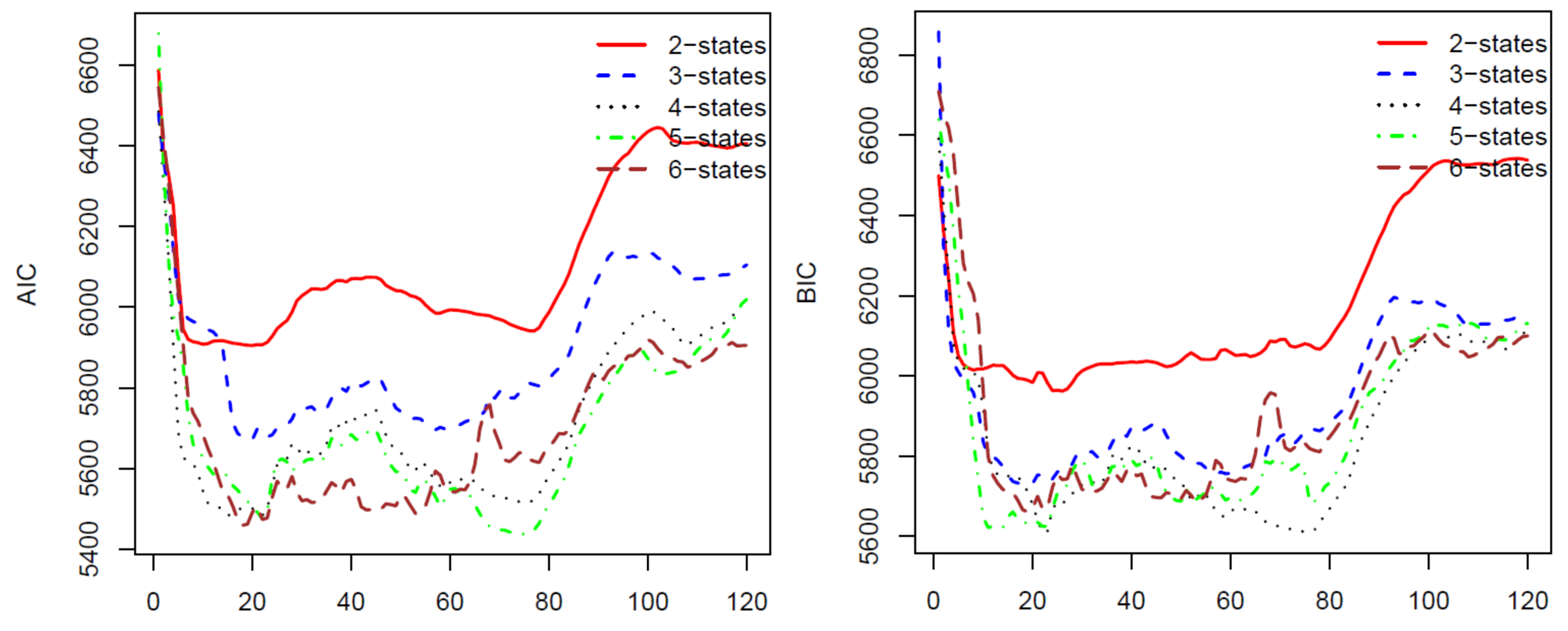
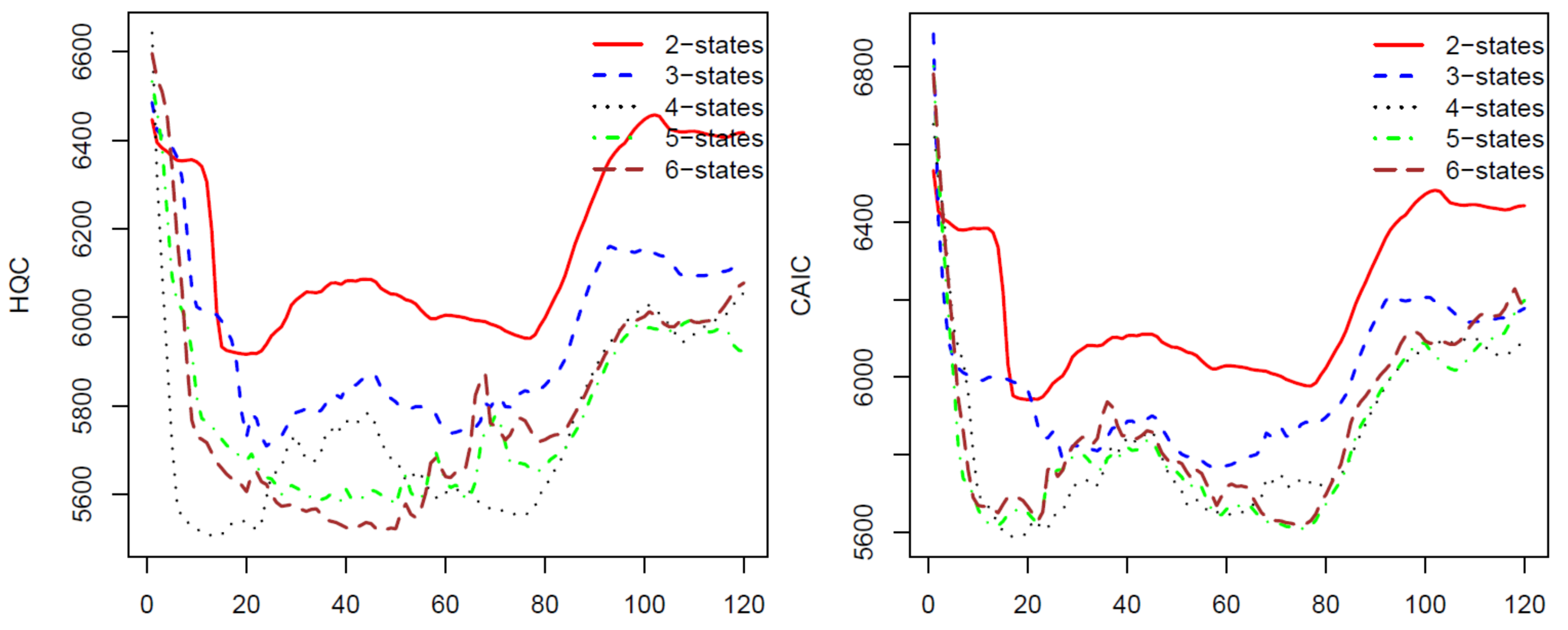
For the second calibration, we move the ten-year data upward one month, we have a new data set from January 1997 to December 2006 and use the calibrated parameters from the first calibration as initial parameters. We repeat the process 120 times for 120 blocks of data by moving the block of data forward. The last block of data is the monthly prices from November 2006 to November 2016. The AIC, BIC, HQC, and CAIC of the 120 calibrations are presented in Figure 1 and Figure 2. In all of these four criteria, a model with a lower criterion value is better. Thus, the results from Figure 1 and Figure 2 show that the four-state HMM is the best model among the two to six state HMMs. Therefore, we will use HMM with four states in stock price predicting and trading. We want to note that, for a different stock using these criteria, we may have another optimal number of states for the HMM. Therefore, we suggest that, before applying the HMM to predict prices for a stock, researchers should use some of the criteria to choose a number of states of the HMM that works the best for the stock.
3.2. Out-of-Sample Stock Price Prediction
In this section, we will use the HMM to predict stock prices and compare the predictions with the real stock prices, and with the results of using the historical average return method. We use S&P 500 monthly prices from January 1950 to November 2016.
We first introduce how to predict stock prices using HMM. The prediction process can be divided into three steps. First, HMM’s parameters are calibrated using training data and the probability is calculated (or likelihood) of the observation of the data set. Then, we will find a “similar data” set in the past that has a similar likelihood to that of the training data. Finally, we will use the difference of stock prices in the last month of the founded sequence with the price of the consecutive month to predict future stock prices. This prediction approach is based on the work of Hassan and Nath (2005). However, the authors predicted daily prices of four airline stocks while we predict monthly prices of the U.S. benchmark market, the S&P 500. Suppose that we want to predict closing price at time of the S&P 500. In the first step, we will choose a fixed time length D of the training data (we call D is the training window) and then use the training data from time to T to calibrate HMM’s parameters, . We assume that the observation probability , defined in Section 1, is Gaussian distribution, so the matrix B, in the parameter , is a two by N matrix of means, , and variances, , of the N normal distributions, where N is the number of states. The initial HMM’s parameters for the calibration were calculated by using formula (5). The training data is the four sequences: open, low, high, and closing price:
We then calculate the probability of observation, . In the second step, we move the block of data backward by one month to have new observation data and calculate . We keep moving blocks of data backward month by month until we find a data set , (), such that . In the final step, we estimate the stock’s closing price for time , , by using the following formula:
Similarly, to predict stock price at time , we will use new training data O: to predict stock price for the time . The calibrated HMM’s parameters in the first prediction were used as the initial parameters for the second prediction. We repeat the three-step-prediction process for the second prediction and so on. For convenience, we use the training window D equal to the out-of-sample forecast period. In practice, we can choose an out-of-sample of any length, but, for the training window D, due to the efficiency of model simulations, we should determine a proper length based on the characteristics of chosen data.
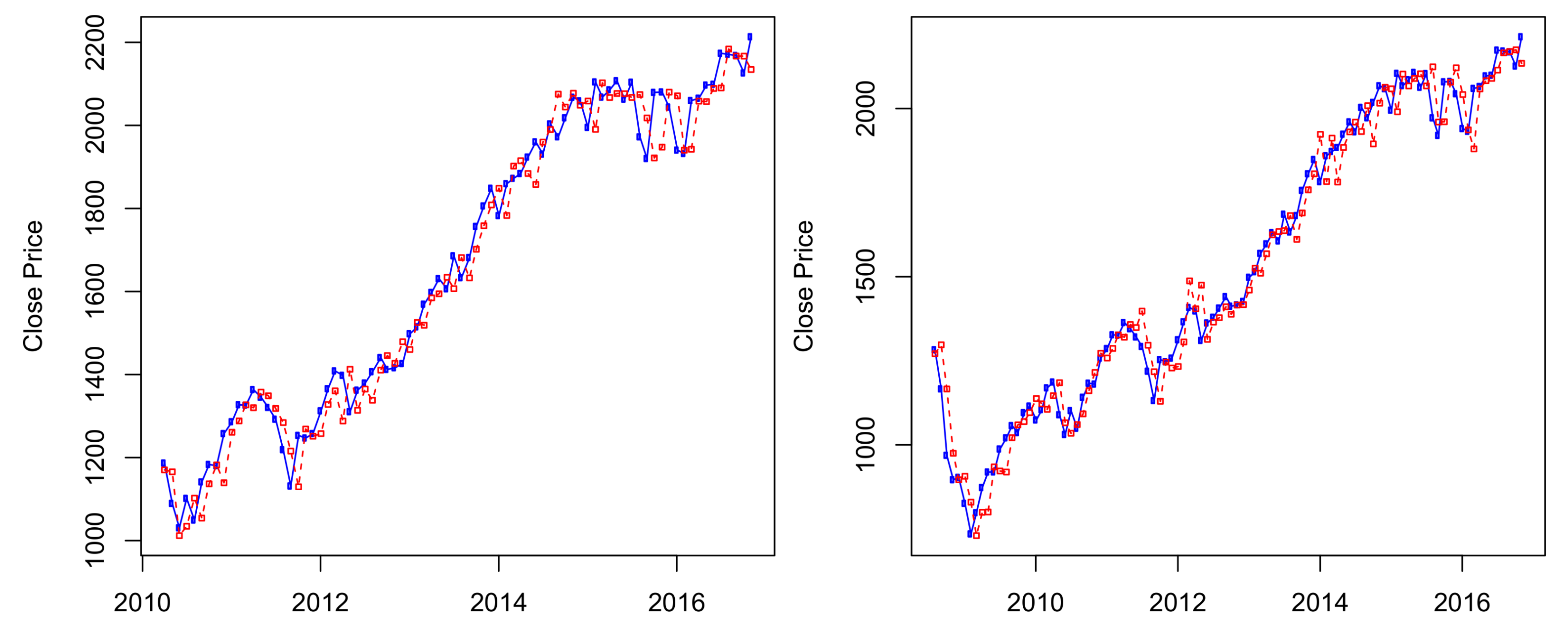
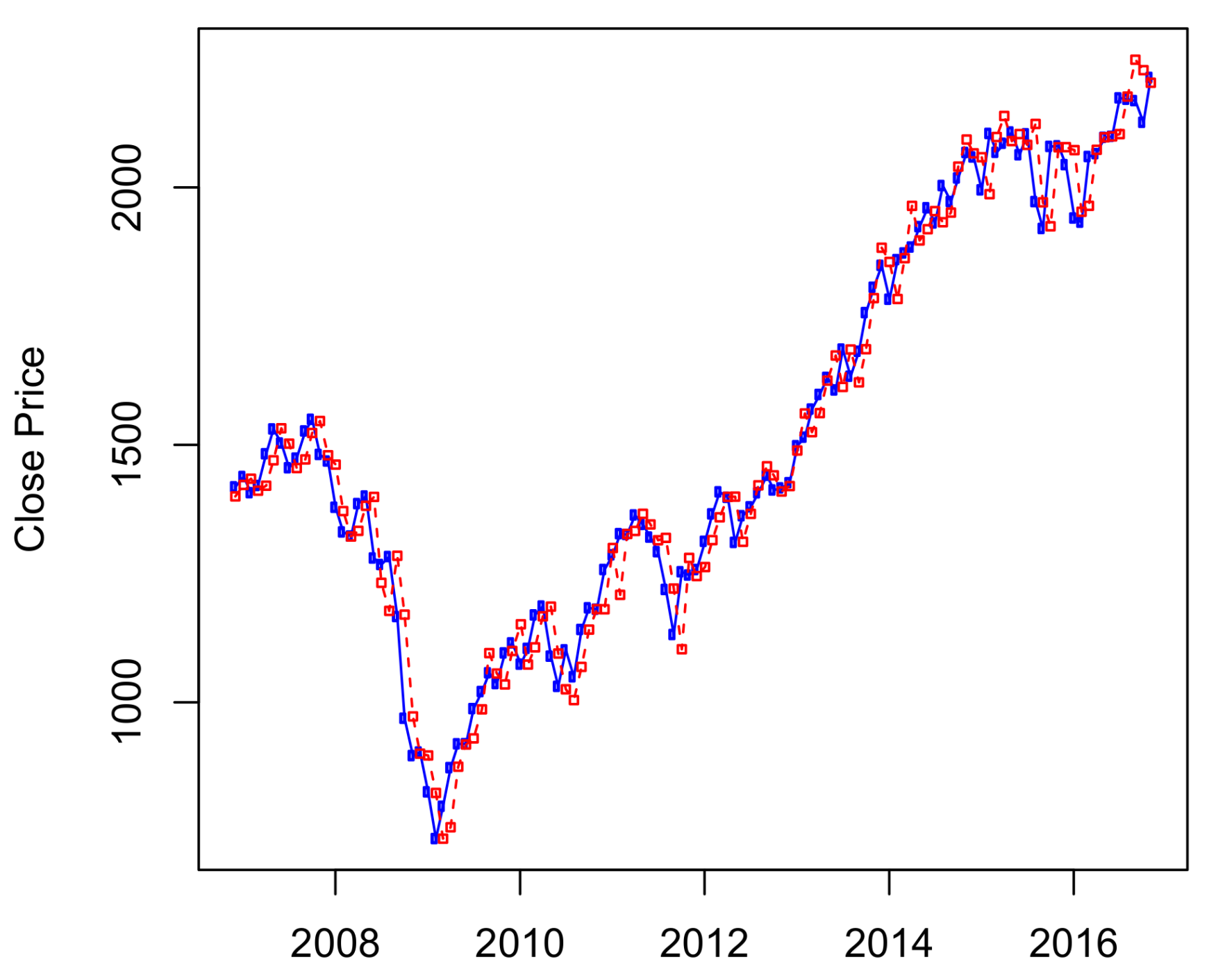
The results of ten-years out-of-sample data () are presented in Figure 3, in which the S&P 500 historical data from January 1950 to October 2006 was used to predict its stock prices from November 2006 to November 2016. We can see from Figure 3 that the HMM captures well the price changes around the economic crisis time from 2008–2009. Results of predictions for other time periods are presented in Figure A1 and Figure A2 of Appendix A.
3.3. Model Validation
To test our predictions, we used the out-of-sample statistics, , introduced by Campbell and Thompson (2008). Many researchers have employed the statistic measure to evaluate their forecasting models. Campbell and Thompson (2008) used the out-of-sample to compare the performances of the stock return prediction model inspired by Welch and Goyal (2008) and that of the historical average return model. The authors used monthly total returns (including dividend) of S&P 500. Rapach et al. (2010) use the out-of-sample to test the efficiency of their combination approach to the out-of-sample equity premium forecasting against the historical average return method. Zhu and Zhu (2013) also used the out-of-sample to show their regime-switching combination forecasts of excess returns gain relative to the historical average model. All of these above approaches were based on a regression model for multi-economic variables to predict stock returns.
The out-of-sample is calculated as follows. First, a time series of returns is divided into two sets: the first m points were called the in-of-sample data set, and the last q points were called the out-of-sample data set. Then, the out-of-sample for forecasted returns is defined as:
where is the real return at time , is the forecasted return from the desired model, and is the forecasted return from the competing model. We can see from the Equation (7) that the evaluates the reduction in the mean squared predictive error (MSPE) of two models. Therefore, if the out-of-sample is positive, then the desired model performed better than the competing model. The historical average return method is used as a benchmark competing model, for which the forecasted return for the next time step is calculated as the average of historical returns up to the time,
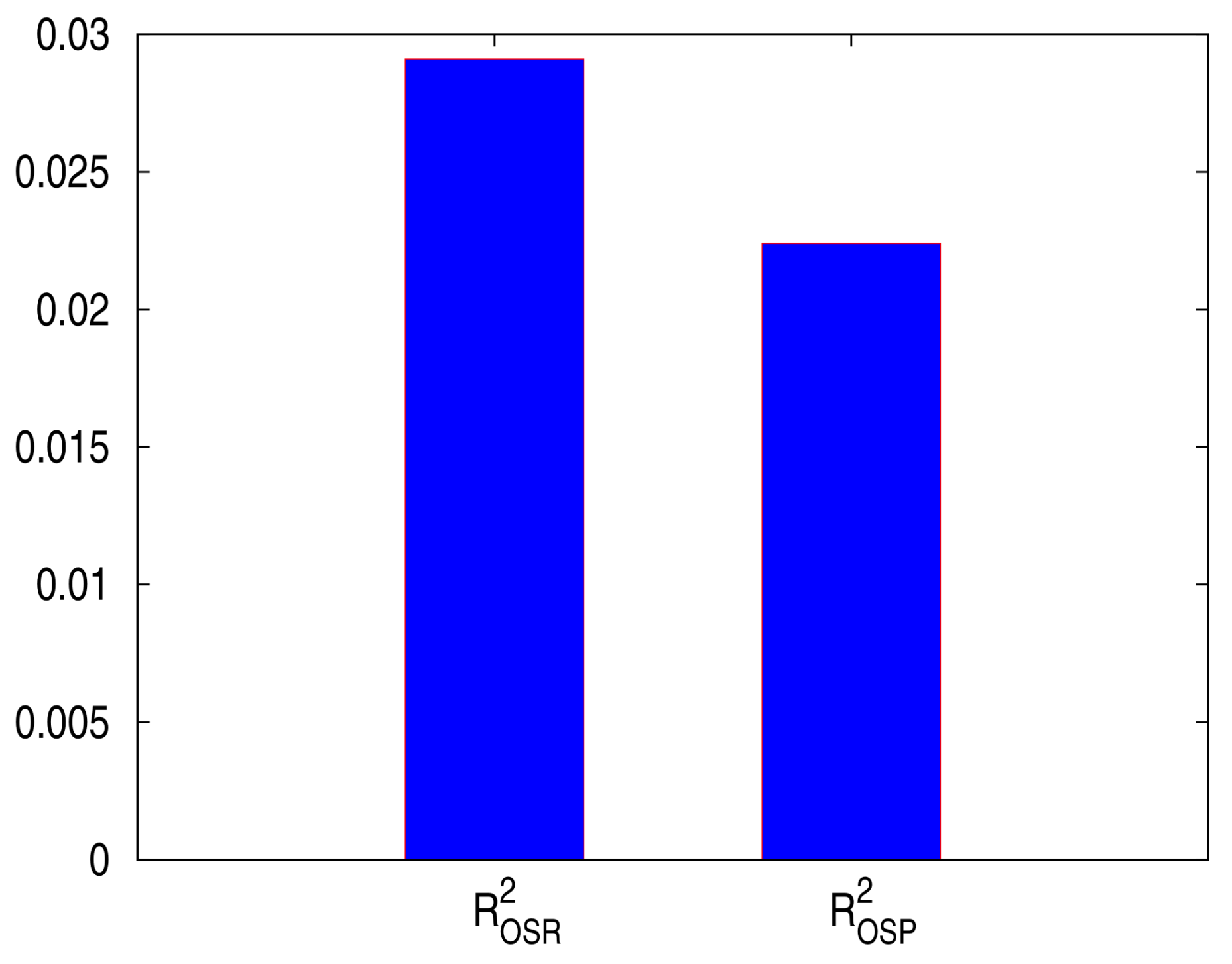
In this study, we use the HMM model to predict stock prices based only on historical prices. However, we can calculate stock prices based on its predicted returns and reverse. Therefore, we will calculate the out-of-sample by using two approaches: out-of-sample for stock returns and out-of-sample for stock prices based on predicted returns (without dividends). Numerical results present in this section are for an out-of-sample and the training periods of the length .
The out-of-sample for relative return (without dividends), namely , is determined by
where is the real relative stock return price at time ,
is the forecasted relative return from the HMM,
and is the forecasted price from the historical average model, . The out-of-sample for stock price based on predicted returns, namely , is given by
where is the real stock price at time , is the forecasted price of the HMM, and is the forecasted price based on the predicted return of the historical average return model,
A positive indicates that the HMM outperforms the historical average model. Therefore, we will use the MSPE-adjusted hypothesized statistics test introduced by Clark and West (2007) to test the null hypothesized versus the alternating hypothesized . In the MSPE-adjusted test, we first define
We then test for (or equal MSPE) by regressing on a constant and using p-value for a zero coefficient. Our p-value for testing and , which are presented in Table 3, are bigger than the efficient level , indicating that we accept the null hypothesis that the coefficient of each test equals zero. Furthermore, the p-values of constants for both tests are significant at level, which imply that we reject the null hypothesized that the and accept the alternating hypothesized that . The out-of-sample for predicted prices and predicted returns are presented in Figure 4, showing that both out-of-sample are positive, i.e., the HMM outperforms the historical average in predicting stock returns and stock prices.
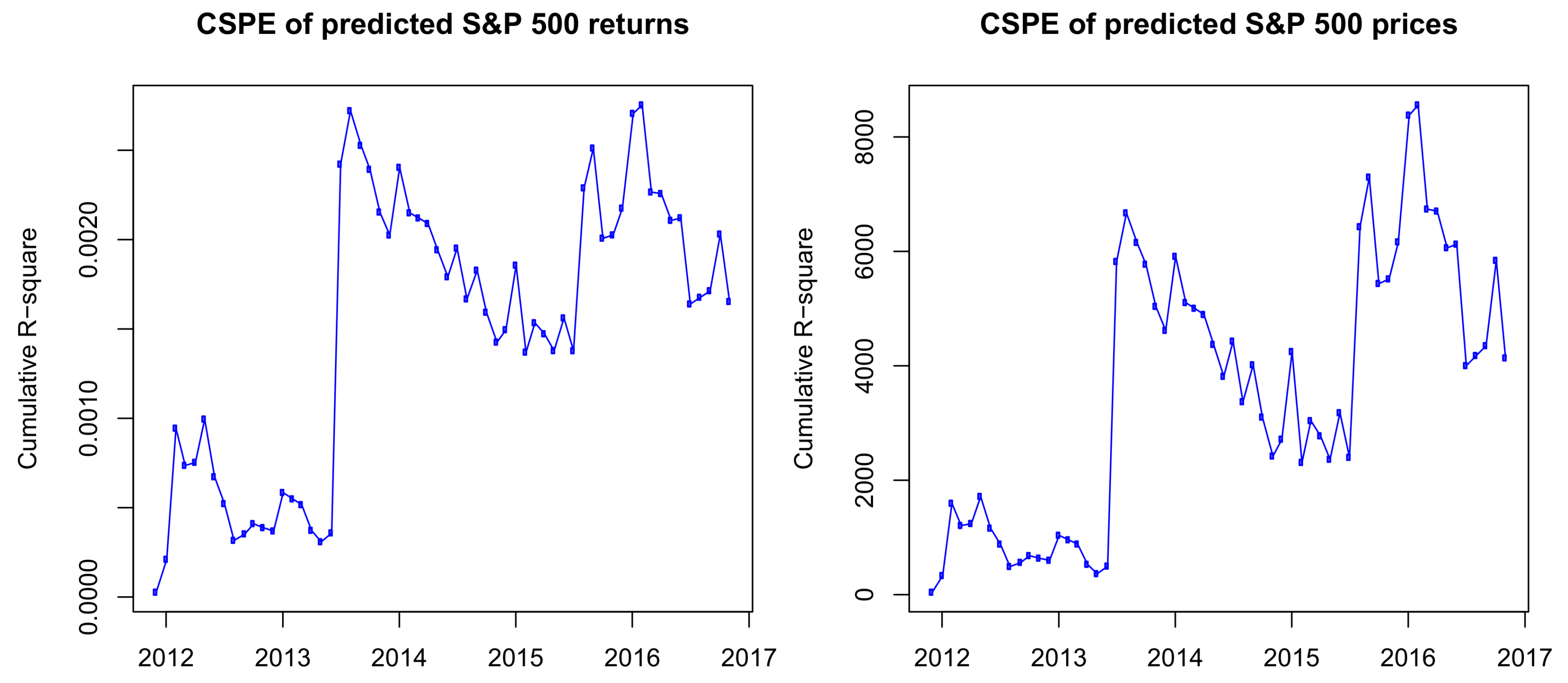
Although the compares the performances of two models on the whole out-of-sample forecasting period, it does not show the efficiency of the two competing models for each point estimation. Therefore, we use the cumulative squared predictive errors (CSPEs), which was presented by Zhu and Zhu (2013), to show the relative performances of the two models after each prediction. The CSPE statistic at time , denoted by CSPE, is calculated as:
From the definition of the cumulative squared predictive errors, we can see that, if the function is increasing, the HMM outperforms the historical average model. In contrast, if the function is decreasing, the historical average model outweighs the HMM on the time interval. If we replace the return prices in Label (12) by the predicted prices, we will have the CSPE for prices. The CSPE of predicted returns and prices is presented in Figure 5.
The results in Figure 5 show that, although in some periods the HAR outperforms the HMM, the CSPEs are positive and follow an uptrend on the whole out-of-sample period. Therefore, we have a conclusion that, in out-of-sample predictions, the HMM outperforms the HAR model.
We also compare the performances of HMM with the historical average model by using the four standard error estimators: the absolute percentage error (APE), the average absolute error (AAE), the average relative percentage error (ARPE) and the root-mean-square error (RMSE). These error estimators are calculated using the following expressions:
where N is a number of simulated points, is the real stock price (or stock return), is the estimated price (or return), and is the mean of the sample. We use the error estimators to calculate the errors of predictions of the HMM and HAR models for predicted returns (Equation (8)) and predicted prices (Equation (10)). Adopting the statistics, we define the efficiency measure to compare the HMM with the HAR model as:
Errors of the two models and the efficiency of the HMM over the HAR are calculated using Equations (13)–(17). A positive efficiency (Eff) indicates that the HMM surpasses the HAR model. Results are presented in Table 4.
Table 4 presents errors and efficiency of HMM over the HAR model. We can see from the table that the HAR model beats the HMM based on the absolute percentage error estimator, APE, for stock returns. However, in all the remaining cases, we have the positive efficiency, which strongly indicates that the HMM outperforms the HAR.
4. Stock Trading with HMM
In this section, we will use the predicted returns of HMM and HAR models to trade S&P 500 using monthly data. If the predicted stock return is positive for the next month, we will buy the stock this month and will sell it if the next predicted return is negative. We assume that we buy and sell with closing prices. If HMM predicts that the stock price will not increase the next month, then we will do nothing. We also assume that the trading cost is $7.00 per trade, this assumption is based on the trading fee on the U.S. market. The trading fees vary from brokers to brokers; some brokers even offer free trading for qualified investors. In reality, we will have many different ways to minimize the transition fee. One simple way is increasing the volume or number of shares in each trading. For each trading, we will buy or sell 100 shares of each of the S&P 500. Based on the results of model selections in Section 2, we only use HMM with four states for the stock trading. We use different training and trading periods to test our model. Trading results of using HMM and HAR models are presented in Table 5.
In Table 5, the “Investment” is the price that we bought 100 shares of the S&P 500 index at the first time. The “Cost” was calculated by multiplying the total numbers of “buy” and “sell” during the period by $7.00. The “Profit” is the percentage of return after trading costs. In the table, we list the trading results of HMM and HAR models, and the Buy & Hold method. In the Buy & Hold technique, we assume that an investor will buy 100 shares of the S&P 500 at the beginning of the trading period and hold it until the end of the period. The results show that the HMM beats the HAR model for all cases and outperforms the Buy & Hold technique for most of the cases except for the 100-month period. In three cases: 40 months, 80 months, and 120 months, the HAR and Buy & Hold models have identical results since all of the HAR’s predicted returns are positive. One disadvantage of the HAR model due to its predictions depend solidly on the mean of historical data, which is not sensitive to a price change at a point. In contrast, HMM captures very well the change of input data at a single point. Therefore, it is more suitable for stock price forecasting than the historical average model.
5. Conclusions
Stock performances are an essential indicator of the strengths and weaknesses of the stock’s corporation and the economy in general. In this paper, we have used the hidden Markov model to predict monthly closing prices of the S&P 500 and then used these predictions to trade the stock. We first use the four criteria: AIC, BIC, HQC, and CAIC to examine the performances of HMM with numbers of states from two to six. The results show that HMM with four states is the best model among these five HMM models. We then use the four-state HMM to predict monthly prices of the S&P 500 and compare this with the results obtained by the benchmark historical average return model. We use the out-of-sample , and other model validation methods to test our model and the results show that the HMM outweighs the historical average method. After validating the HMM model for out-of-sample predictions, we apply the model to trade the S&P 500 using different training and testing periods. The numerical results show that the four-state HMM outperforms the HAR not only in return predictions, but also in stock trading. Overall, the HMM model beats the Buy & Hold strategy and yields higher percentage returns. The testing and trading results indicate that the HMM is the potential model for stock price predictions and stock trading.
Acknowledgments
We thank a co-editor and four anonymous referees for their valuable comments and suggestions.
Conflicts of Interest
The author declares no conflict of interest.
Appendix A. Algorithms
Appendix A.1. Forward Algorithm
We define the joint probability function as
and then we calculate recursively. The probability of observation is just the sum of the .
| Algorithm A1: The forward Algorithm. |
|
Appendix A.2. Backward Algorithm
| Algorithm A2: The backward algorithm. |
|
Appendix A.3. Baum–Welch Algorithm
In order to describe the procedure, we define the conditional probability
for . Obviously, for , and we have the following backward recursive relation
| Algorithm A3: Baum–Welch for L independent observations with the same length T. |
|
We then defined , the probability of being in state at time t of the observation as:
The probability of being in state at time t and state at time of the observation as:
Clearly,
Note that the parameter was updated in Step 2 of the Baum–Welch algorithm to maximize the function so we will have .
If the observation probability , defined in Section 1, is Gaussian, we will use the following formula to update the model parameter,
Appendix A.4. S&P 500’s Price Prediction Results
Figure A1.
S&P 500 ’s predicted prices using the four-state HMM for 40-month out-of-sample period (left) and 60-month out-of-sample period (right).
Figure A1.
S&P 500 ’s predicted prices using the four-state HMM for 40-month out-of-sample period (left) and 60-month out-of-sample period (right).
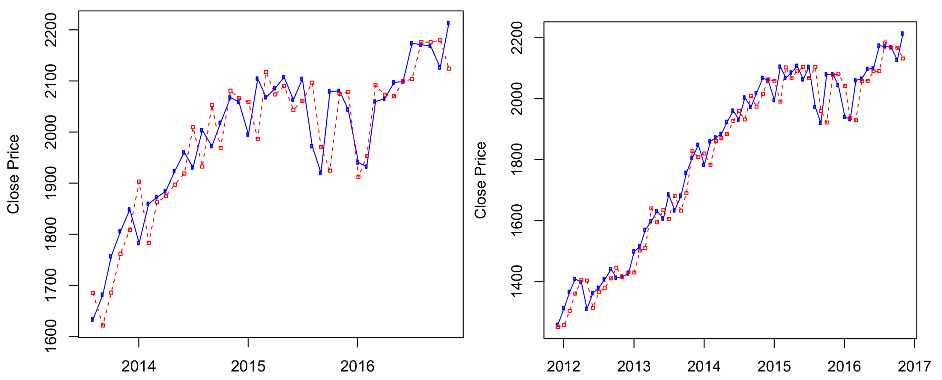
Figure A2.
S&P 500 ’s predicted prices using the four-state HMM for 80-month out-of-sample period (left) and 100-month out-of-sample period (right).
Figure A2.
S&P 500 ’s predicted prices using the four-state HMM for 80-month out-of-sample period (left) and 100-month out-of-sample period (right).
References
- Akaike, Hirotugu. 1974. A new look at the statistical model identification. IEEE Transactions on Automatic Control 19: 716–23. [Google Scholar] [CrossRef]
- Ang, Andrew, and Geert Bekaert. 2002. International Asset Allocation with Regime Shifts. The Review of Financial Studies 15: 1137–87. [Google Scholar] [CrossRef]
- Baum, Leonard E., and John Alonzo Eagon. 1967. An inequality with applications to statistical estimation for probabilistic functions of Markov process and to a model for ecology. Bulletin of the American Mathematical Society 73: 360–63. [Google Scholar] [CrossRef]
- Baum, Leonard E., and George Sell. 1968. Growth functions for transformations on manifolds. Pacific Journal of Mathematics 27: 211–27. [Google Scholar] [CrossRef]
- Baum, Leonard E., and Ted Petrie. 1966. Statistical inference for probabilistic functions of finite state Markov chains. The Annals of Mathematical Statistics 37: 1554–63. [Google Scholar] [CrossRef]
- Baum, Leonard E., Ted Petrie, George Soules, and Norman Weiss. 1970. A maximization technique occurring in the statistical analysis of probabilistic functions of Markov chains. The Annals of Mathematical Statistics 41: 164–71. [Google Scholar] [CrossRef]
- Bozdogan, Hamparsum. 1987. Model selection and Akaike’s Information Criterion (AIC): the general theory and its analytical extensions. Psychometrika 52: 345–70. [Google Scholar] [CrossRef]
- Campbell, John Y., and Samuel B. Thompson. 2008. Predicting the Equity Premium Out of Sample: Can Anything Beat the Historical Average? Review of Financial Studies 21: 1509–31. [Google Scholar] [CrossRef]
- Clark, Todd E., and Kenneth D. West. 2007. Approximately normal tests for equal predictive accuracy in nested models. Journal of Econometrics 138: 291–311. [Google Scholar] [CrossRef]
- Erlwein, Christina, Rogemar Mamon, and Matt Davison. 2009. An Examination of HMM-based Investment Strategies for Asset Allocation. Applied Stochastic Models in Business and Industry 27: 204–21. [Google Scholar] [CrossRef]
- Guidolin, Massimo, and Allan Timmermann. 2007. Asset allocation under multivariate regime switching. Journal of Economic Dynamics and Control 31: 3503–44. [Google Scholar] [CrossRef]
- Hamilton, James D. 1989. A New Approach to the Economic Analysis of Nonstationary Time Series and the Business Cycle. Econometrica 57: 357–84. [Google Scholar] [CrossRef]
- Hannan, Edward J., and Barry G. Quinn. 1979. The determination of the order of an autoregression. Journal of the Royal Statistical Society. Series B (Methodological) 41: 190–95. [Google Scholar]
- Hassan, Md Rafiul, and Baikunth Nath. 2005. Stock Market Forecasting Using Hidden Markov Models: A New Approach. In Paper presented at Proceedings of the IEEE fifth International Conference on Intelligent Systems Design and Applications, Wroclaw, Poland, September 8–10; pp. 192–96. [Google Scholar]
- Honda, Toshiki. 2003. Optimal Portfolio Choice for Unobservable and Regime-switching Mean Returns. Journal of Economic Dynamics and Control 28: 45–78. [Google Scholar] [CrossRef]
- Kritzman, Mark, Sebastien Page, and David Turkington. 2012. Regime Shifts: Implications for Dynamic Strategies. Financial Analysts Journal 68: 22–39. [Google Scholar] [CrossRef]
- Levinson, Stephen E., Lawrence R. Rabiner, and Man Mohan Sondhi. 1983. An introduction to the application of the theory of probabilistic functions of Markov process to automatic speech recognition. The Bell System Technical Journal 62: 1035–74. [Google Scholar] [CrossRef]
- Li, Xiaolin, Marc Parizeau, and Réjean Plamondon. 2000. Training Hidden Markov Models with Multiple Observations—A Combinatorial Method. IEEE Transactions on Pattern Analysis and Machine Intelligence 22: 371–77. [Google Scholar]
- Nguyen, Nguyet Thi. 2014. Probabilistic Methods in Estimation and Prediction of Financial Models. PhD thesis, Florida State University, Tallahassee, FL, USA. [Google Scholar]
- Nguyen, Nguyet, and Dung Nguyen. 2015. Hidden Markov Model for Stock Selection. Risks 3: 455–73. [Google Scholar] [CrossRef]
- Gupta, Aditya, and Dhingra Bhuwan. 2012. Stock market prediction using Hidden Markov models. In Paper presented at Proceedings of the Student Conference on Engg and Systems (SCES), Allahabad, Uttar Pradesh, India, March 16–18; pp. 1–4. [Google Scholar]
- Rabiner, Lawrence R. 1989. A Tutorial on Hidden Markov Models and Selected Applications in Speech Recognition. Proceedings of the IEEE 77: 257–86. [Google Scholar] [CrossRef]
- Rapach, David E., Jack K. Strauss, and Guofu Zhou. 2010. Out-of-Sample Equity Premium Prediction: Combination Forecasts and Links to the Real Economy. The Review of Financial Studies 23: 821–62. [Google Scholar] [CrossRef]
- Sass, Jörn, and Ulrich G. Haussmann. 2004. Optimizing the Terminal Wealth under Partial Information: The Drift Process as A Continuous Time Markov Chain. Finance and Stochastic 8: 553–77. [Google Scholar] [CrossRef]
- Schwarz, Gideon. 1978. Estimating the Dimension of A Model. The annals of statistics 6: 461–64. [Google Scholar] [CrossRef]
- Taksar, Michael, and Xudong Zeng. 2007. Optimal Terminal Wealth under Partial Information: Both the Drift and the Volatility Driven by a Discrete-time Markov Chain. SIAM Journal on Control and Optimization 46: 1461–82. [Google Scholar] [CrossRef]
- Viterbi, Andrew. 1967. Error Bounds for Convolutional Codes and An Asymptotically Pptimal Decoding Algorithm. IEEE transactions on Information Theory 13: 260–69. [Google Scholar] [CrossRef]
- Welch, Ivo, and Amit Goyal. 2008. A Comprehensive Look at the Empirical Performance of Equity Premium Prediction. The Review of Financial Studies 21: 1455–508. [Google Scholar] [CrossRef]
- Zhu, Xiaoneng, and Jie Zhu. 2013. Predicting Stock Returns: A Regime-Switching Combination Approach and Economic Links. Journal of Banking and Finance 37: 4120–33. [Google Scholar]
- Geweke, John, and Nobuhiko Terui. 1993. Bayesian Threshold Autoregressive Models for Nonlinear Time Series. Journal of Time Series Analysis 14: 441–54. [Google Scholar] [CrossRef]
- Frühwirth-Schnatter, Sylvia. 2006. Finite Mixture and Markov Switching Models. Berlin: Springer. [Google Scholar]
- Juang, Biing-Hwang, and Lawrence Rabiner. 1985. Mixture autoregressive hidden Markov models for speech signals. IEEE Transactions and Acoustic, Speech, and Signal Processing 33: 1404–13. [Google Scholar] [CrossRef]
- Wong, Chun Shan, and Wai Keung Li. 2000. On a Mixture Autoregressive Model. Journal of the Royal Statistical Society, Series B 62: 95–115. [Google Scholar] [CrossRef]
Figure 1.
AIC (left) and BIC (right) for 120 HMM’s parameter calibrations using S&P 500 monthly prices.
Figure 1.
AIC (left) and BIC (right) for 120 HMM’s parameter calibrations using S&P 500 monthly prices.

Figure 2.
HQC (left) and CAIC (right) for 120 HMM’s parameter calibrations using S&P 500 monthly prices.
Figure 2.
HQC (left) and CAIC (right) for 120 HMM’s parameter calibrations using S&P 500 monthly prices.

Figure 3.
Predicted S&P 500 monthly prices from November 2006 to November 2016 using four-state HMM.
Figure 3.
Predicted S&P 500 monthly prices from November 2006 to November 2016 using four-state HMM.

Figure 4.
The , and of S&P 500 monthly prices from December 2011 to November 2016.

Figure 5.
Cumulative squared predictive errors, CSPE, of S&P 500 monthly forecasted prices (right) and returns (left) from December 2011 to November 2016.
Figure 5.
Cumulative squared predictive errors, CSPE, of S&P 500 monthly forecasted prices (right) and returns (left) from December 2011 to November 2016.


Table 1.
The basic elements of a hidden Markov model.
| Element | Notation/Definition |
|---|---|
| Length of observation data | T |
| Number of states | N |
| Number of symbols per state | M |
| Observation sequence | |
| Hidden state sequence | |
| Possible values of each state | |
| Possible symbols per state | |
| Transition matrix | , |
| Vector of initial probability of being in state (regime) at time | , |
| Observation probability matrix | , and |
Table 2.
Summary of S&P 500 index monthly prices from 1 March 1950 to 11 January 2016.
| Price | Min | Max | Mean | Std. |
|---|---|---|---|---|
| Open | 16.66 | 2173.15 | 504.06 | 582.20 |
| High | 17.09 | 2213.35 | 520.46 | 599.28 |
| Low | 16.66 | 2147.56 | 486.91 | 562.96 |
| Close | 17.05 | 2213.35 | 506.73 | 584.98 |
Table 3.
The mean squared predictive error adjusted test, MSPE-adj, for and .
| MSPE-adj. | Coefficients | Estimate | Std. Error | t-Statistics | p-Value | |
|---|---|---|---|---|---|---|
| Intercept | *** | |||||
| 0.921 | ||||||
| Intercept | *** | |||||
| 0.938 |
Note: ‘***’ indicates that the test result is significant at the 0.001 level.
Table 4.
Error and efficiency of S&P 500’s predicted prices and predicted returns using the HMM versus HAR model.
Table 4.
Error and efficiency of S&P 500’s predicted prices and predicted returns using the HMM versus HAR model.
| Error Estimators | APE | AAE | ARPE | RMSE | |
|---|---|---|---|---|---|
| Predicted Return | HMM | 0.3325 | 0.0245 | 0.0303 | 2.4371 |
| HAR | 0.1708 | 0.0249 | 0.0308 | 2.4752 | |
| Eff. | −0.9467 | 0.0161 | 0.0161 | 0.0154 | |
| Predicted Price | HMM | 0.0242 | 43.5080 | 54.8606 | 0.0240 |
| HAR | 0.0246 | 44.2091 | 55.4853 | 0.02440 | |
| Eff. | 0.0163 | 0.0159 | 0.0113 | 0.0164 |
Table 5.
S&P 500 trading using the HMM, HAR, and Buy & Hold models for different time periods.
| Trading Period | Model | Investment ($) | Earning ($) | Cost ($) | Profit (%) |
|---|---|---|---|---|---|
| 40 months | HMM | 168,155 | 65,172 | 168 | 38.66 |
| (7/2013 | HAR | 168,573 | 52,762 | 14 | 31.29 |
| –11/2016) | Buy & Hold | 168,573 | 52,762 | 14 | 31.29 |
| 60 months | HMM | 124,696 | 95,205 | 378 | 76.05 |
| (12/2011 | HAR | 131,241 | 90,094 | 14 | 68.64 |
| –11/2016) | Buy & Hold | 124,696 | 96,639 | 14 | 77.49 |
| 80 months | HMM | 116,943 | 113,971 | 392 | 97.12 |
| (4/2010 | HAR | 116,943 | 104,392 | 14 | 89.26 |
| –11/2016) | Buy & Hold | 116,943 | 104,392 | 14 | 89.26 |
| 100 months | HMM | 126,738 | 94282 | 616 | 73.91 |
| (8/2008 | MAR | 126,738 | 73,010 | 84 | 57.54 |
| –11/2016) | Buy & Hold | 126,738 | 94,597 | 14 | 74.63 |
| 120 months | HMM | 141,830 | 100,614 | 770 | 70.39 |
| (11/2006 | HAR | 140,063 | 81,272 | 14 | 58.15 |
| –11/2016) | Buy & Hold | 140,063 | 81,272 | 14 | 58.15 |
© 2018 by the author. Licensee MDPI, Basel, Switzerland. This article is an open access article distributed under the terms and conditions of the Creative Commons Attribution (CC BY) license (http://creativecommons.org/licenses/by/4.0/).
Share and Cite
MDPI and ACS Style
Nguyen, N. Hidden Markov Model for Stock Trading. Int. J. Financial Stud. 2018, 6, 36. https://doi.org/10.3390/ijfs6020036
AMA Style
Nguyen N. Hidden Markov Model for Stock Trading. International Journal of Financial Studies. 2018; 6(2):36. https://doi.org/10.3390/ijfs6020036
Chicago/Turabian StyleNguyen, Nguyet. 2018. "Hidden Markov Model for Stock Trading" International Journal of Financial Studies 6, no. 2: 36. https://doi.org/10.3390/ijfs6020036
Note that from the first issue of 2016, this journal uses article numbers instead of page numbers. See further details here.