An Empirical Investigation of Risk-Return Relations in Chinese Equity Markets: Evidence from Aggregate and Sectoral Data


1
Department of Finance, Drexel University, LeBow Hall, 3220 Market Street, Philadelphia, PA 19104, USA
2
China Securities, Beijing Anli Sales Office, Tower C, Anli Garden, 66 Anli Street, ChaoYang District, Beijing 10020, China
*
Author to whom correspondence should be addressed.
Int. J. Financial Stud. 2018, 6(2), 35; https://doi.org/10.3390/ijfs6020035
Submission received: 10 December 2017
/
Revised: 14 March 2018
/
Accepted: 14 March 2018
/
Published: 26 March 2018
(This article belongs to the Special Issue Finance, Financial Risk Management and their Applications)
Abstract
:This paper investigates the risk-return relations in Chinese equity markets. Based on a TARCH-M model, evidence shows that stock returns are positively correlated with predictable volatility, supporting the risk-return relation in both aggregate and sectoral markets. Evidence finds a positive relation between stock return and intertemporal downside risk, while controlling for sentiment and liquidity. This study suggests that the U.S. stress risk or the world downside risk should be priced into the Chinese stocks. The paper concludes that the risk-return tradeoff is present in the GARCH-in-mean, local downside risk-return, and global risk-return relations.
JEL Classification:
G11; G12; G151. Introduction
Merton’s (1973) pioneering research on intertemporal capital asset pricing model (ICAPM) posits a positive risk-return relation in asset markets. In line with Merton’s work, a substantial number of research papers have studied whether investments in higher risk assets are rewarded by higher returns. In conducting empirical analysis, conditional variance, a methodology proposed by Engle (1982, 2009)1, has been commonly used to test the relation between risk and stock returns. French et al. (1987) use this method to test the U.S. equity market and find evidence that the expected excess stock return is positively related to the predictable conditional volatility of stock returns. Subsequent studies by Bali and Peng (2006) and Bekaert et al. (2007) reach a similar qualitative conclusion. However, contrary results are found in the studies of Nelson (1991) and Glosten et al. (1993). Therefore, the literature reaches no agreement on the risk-return relation.
A key issue faced by researchers is the lack of a concise way to measure risk, which is often subject to the rationale of researchers who use a certain set of information to justify their approach. Concern has also been expressed on whether a Gaussian-type GARCH (Engle 1995, 2009) model is an appropriate procedure to derive the conditional variance for examining the risk-return relation, especially in its ability to test the null in a highly volatile environment. To address whether asset returns often exhibit heavier tails and asymmetric impact on variance, research (Harvey and Siddique 1999; Peiro 1999) has moved in the direction of including higher moments such as skewness and kurtosis (Scott and Horvath 1980; Harvey and Siddique 1999; Harvey et al. 2010; Chiang and Li 2013).
The financial crisis period of 2007–2008 suggests that investors’ risk averse behavior cannot sufficiently be described by conditional variance when a market encounters extreme price shocks. Worried about a big financial loss, investors would shift their behavior, making safety a first priority. For this reason, VaR becomes an appealing variable for investors and industry managers applying to the downside-risk analysis (Bali et al. 2009; Chen and Chiang 2016b).
The above empirical works have frequently been dedicated to the U.S. markets or other industrial countries; however, very little attention has been given to the Chinese stock market for several reasons. First, despite its impressive economic growth and accumulation of international reserves, China is considered a latecomer as compared with other financial markets typically referred to as developed. Thus, very few investment instruments are available to investors. Most Chinese investors know very little about sophisticated investment strategies; therefore, their behavior is more likely reactions to indicators of government policies or regulations. Second, researchers occasionally face a shortage-of-data problem when conducting empirical research in Chinese financial markets, encountering either a lack of data or limitations in the length of historical data (Rojas-Suarez 2014; Chen and Chiang 2016a). As a result, principles of financial market behavior and microstructure entailed in advanced markets cannot be directly applied or used to investigate the China market.
China’s persistent growth over the years has helped to accumulate a large amount of international reserves, which provide a considerable supply of loanable funds, demanding for the instruments of investments. Moreover, the Chinese government in recent years has been more liberal in conducting its financial policy. For example, the “stock connects” link between the Shanghai–Hong Kong stock exchanges and, recently, the Shenzhen–Hong Kong stock exchanges have removed the traditional restrictions on holding stocks across national borders by international institutional investors. For local Chinese households, these schemes provide more investment outlets and instruments to satisfy households’ saving plans; without these outlets, their investments would mainly target the real estate market (Chiang and Chen 2016b; Borst 2017).
On 30 November 2015, China’s Renminbi (RMB) was designated as one of the world’s key currency by the International Monetary Fund (IMF) (Lagarde 2015), a move that underscores the China’s rising financial and economic influence.2 This decision will give a broader use of the RMB in world trading and financial transactions. To meet the IMF’s provision, China will forcefully give up some of its freedom on currency policy and absorb some exchange rate volatility from international markets. These new developments provide fresh opportunities to examine the risk-return relation in the Chinese markets.3 This empirical analysis, if successful, will not only inform investors about their investment decision but also policymakers who need to maintain financial market stability.
Motivated by the above issues, we specify a model that focuses on three different measures of risk. The first is the risk-return relation using the conventional approach proposed in the GARCH-M model (French et al. 1987; Li 2007; Engle 2009; Cheng et al. 2014). This approach highlights that higher stock returns are associated with high expected variances. The second is downside risk measured by VaR, which accounts for the extreme market worsening and was selected over the conditional variance that does not give enough weight to the impact of extreme downside price movements. This line of empirical analysis can provide more insight into the market disturbance arising from an unexpected daily extreme shock. The third is the contagion risk that takes place as a financial crisis spreads in financial centers and causes investors to assess their portfolios vis-à-vis a similar class of investments in other countries (Forbes and Rigobon 2002; Pericoli and Sbracia 2003; Chiang et al. 2007). This effect appears to have a more profound influence on emerging markets (Bekaert et al. 1998; Bekaert et al. 2007). Although the Chinese market was able to escape a big financial loss during the Asian crisis in 1997–1998, the damage from the world financial crisis in 2007–2008 was tremendous. As a result, it is worth examining the risk from an external source on Chinese stock returns.
The remainder of this paper is organized as follows. Section 2 provides a brief review of the literature on risk-return relations. Section 3 presents a TARCH-M model to examine risk-return relations. Section 4 discusses the variables in this study. Section 5 describes the data and discusses related statistics. Section 6 presents estimated equations in both the aggregate market and sectoral level. Section 7 contains a summary of the study.
2. Literature Review
Merton (1973, 1980) developed an intertemporal CAPM (ICAPM) model that shows a positive relation between expected excess returns and risk4, and can be expressed by:
where (= is the excess return of the market portfolio at time t; is an expectation operator at time t − 1; is the relative risk aversion parameter of the representative agent; and is the market return variance at time t, which is considered a proxy for risk (Bali and Peng 2006). While testing that = 0, French et al. (1987), Baillie and DeGennaro (1990), Ghysels et al. (2005), Bali and Peng (2006), and Bali and Cakici (2010) find evidence of a positive, statistically significant relation. However, Nelson (1991) and Glosten et al. (1993), who tested the same hypothesis, report that the expression had a negative relation. The reason for a difference in sign may stem from the sample period, the methods (models and exogenous variables) used, or the inclusion/exclusion of certain control variables (Lettau and Ludvigson 2010).
Because some investors are more inclined to tackle the downside risk-return relation after suffering from a big financial loss during a financial crisis, some researchers have focused on studying the impact of the downside risk on stock returns using:
where is the price of downside risk, is the expected VaR of the market portfolio, which is usually obtained from the conditional VaR daily (monthly) index returns. In the empirical analysis, the conditional VaR is approximated by either the realized or the lagged realized VaR, or generated by a GARCH-type model (Bali et al. 2009).
Using VaR to measure downside risk, Bali and Cakici (2010) find that a VaR can explain the cross-sectional variation in expected returns. The positive relation between average returns and the VaR is robust for different investment horizons. Testing the data in the time-series, they find supporting evidence for using VaR in predicting stock returns after controlling for size, the book-to-market ratio and liquidity. Further testing of U.S. monthly data for the sample period of January 1926–December 2005, Bali et al. (2009) confirm an intertemporal relation between expected stock returns and the VaR. In their investigation of G7 markets, Chen and Chiang (2016b) document that a positive intertemporal risk-return relation is persistently present during an ordinary volatility regime. However, as uncertainty rises, there is an increased probability that the positive risk-return relation will gradually move to the high-volatility regime and the sign of the risk-return relation will turns negative. This finding implies that the estimated results are subject to two different regimes on the level of risk, indicating that and may serve two different sets of informational content that investors use to make decisions on their investments. Thus, it is relevant to use both variables, and the as different arguments to explain stock returns. This notion can be expressed as:
where A and B are constant parameters. In the empirical estimation, it is sufficient to equate the realized value to the expected value plus an error term. In addition, the control variables are usually added to the test equation to avoid a spurious correlation.
3. A Basic Model in Empirical Analysis
Following the previous discussions, we specify China’s stock return, , as a linear function of a few key financial variables that are expressed as:
if and 0 otherwise.
where , , and
Equation (4) is the mean equation and is the market (or excess) stock return. refers to GARCH-in-mean. This basic model’s result indicates that a higher stock return is expected if there is a higher expected volatility denoted by conditional standard deviation. suggests that a higher return is anticipated in the next period if a downside risk is expected to be higher. If this were the case, a downside risk–return relation tradeoff would be indicated. The means undecided restriction, depending on control variables, , being included, such as investment sentiment (Baker and Wurgler 2006; Baker and Wurgler 2007) or market liquidity (Cooper et al. 1985; Domowitz et al. 2005; Pastor and Stambaugh 2003), among others. Equation (5) is a variance equation following the Threshold (GJR)-GARCH process (Chiang and Doong 2001).5 In this model, we add a volatility asymmetric term to indicate that bad news, < 0, will have a more profound impact on volatility, , than good news, > 0. In empirical estimations, we follow Bollerslev et al. (1992) by assuming p = q = k = 1 in Equation (5). That is, good news has an impact of , while bad news has an impact of . As such when , bad news increases volatility.
In Equation (4), stock return in the Chinese market, , is specified as a positive and a linear function of the conditional standard deviation, , a lagged extreme downside price change, changes in the investment sentiment () and market liquidity of stocks ( (Elyasiani et al. 2000; Bekaert et al. 2007) in the lagged one period.6
Equation (5), which describes the evolution of conditional volatility for a stock return and follows a Threshold GARCH(1,1)-M process (TARCH(1,1)-M) (see Engle 1982; Bollerslev 1986; Glosten et al. 1993; Chiang and Doong 2001), assumes that the conditional variance, , is generated by the past shock squared and the lagged conditional variance plus an asymmetric effect due to negative news. Thus, Equation (5) captures not only the volatility clustering phenomenon, but also the asymmetrical impact of news on the conditional variance.7 Our prior empirical experiments suggest that Equation (5) with TARCH(1,1)-M model sufficiently captures the conditional variance of returns in the Chinese stock market.
Equation (6) is modeled as a generalized error distribution (GED) (Nelson 1991). This distribution is appealing, since the error series can be smoothly transformed from a normal distribution into a leptokurtotic distribution (fat tails) or even into a platykurtotic distribution (thin tails).8 Gao et al. (2012) compare GARCH models based on different distributions with the MCMC method and conclude that GED-GARCH is the best model to describe China’s stock market volatility. Because the GED adequately accommodates the thickness of the tails of a distribution and we later find that the conditional variance displays significant power in predicting stock returns, it can be argued that the GED-TARCH-M model has the best fit for the Chinese stock return series.
4. Selection of Variables
To conduct empirical estimations of the Chinese stock return equations, we focus on two sets of variables, which serve as regressors: They are (i) risk variables that reflect stock return variations and (ii) variables for measuring market liquidity and investors’ sentiments. The selection of explanatory variables is based on economic rationales and prior empirical regularities of the variable of interest. The specifications of the variable measurement and the forms of the variable transformation depend mainly on the time-series properties and sometimes are the result of empirical experiments. Their specification also depends on prior beliefs as to whether the variables are meaningful enough to be included. For these reasons, the growth of the dividend yield was deleted because its t-value is insignificant (Fama and French 1988; Campbell and Shiller 1988a; Campbell and Shiller 1988b; Campbell et al. 1997), and interest rates are excluded because they lack variations due to government manipulation.
(1) Expected volatility. Expected volatility, which follows a TARCH(1,1)-M process (Bollerslev 1986; Glosten et al. 1993; Chiang and Doong 2001), is generated by using Equation (5), which describes the evolution of a conditional volatility of stock returns. It assumes that the conditional variance, , is generated by the past shock squared and the lagged conditional variance plus an asymmetric effect following negative news.9 Our prior empirical experiments suggest that Equation (5) with the TARCH(1,1)-M model sufficiently captures the feature of the conditional variance of returns in Chinese stocks.
(2) Downside risk. The downside price change is obtained from the lowest daily stock return based on the left tail of the actual daily stock return distribution. Following Bali et al. (2009), we choose the lowest value among 21 daily returns times −1 to form monthly downside risk. This measure is equivalent to the concept of VaR proposed by Bali et al. (2009). Thus, the estimated slope of the lagged downside risk provides empirical justification of the downside risk-return relation from daily activities, while the slope of the conditional volatility helps to identify the effect of conditional variance arising from monthly data. The procedure to derive the downside risk applies to both the Chinese market and world market.
(3) Global financial risk—STLFSI. The construction of the STLFSI (Federal Reserve Bank of St. Louis 2014) is based on weekly information of 18 individual financial variables, including seven interest rates (the effective federal funds rate, the Treasury bill rate, Baa-rated corporate bonds, Merrill Lynch Asset-Backed Master BBB-rated), six yield spreads (the yield curve, corporate Baa-rated bond minus the 10-year Treasury, TED), and five other indicators (Chicago Board Options Exchange Market Volatility Index [VIX], Merrill Lynch Bond Market Volatility Index (1-month)).10 Each of these financial variables represents some sort of financial stress on bond or equity markets. Since this financial stress index is based on the first principal component for explaining the co-movement of the 18 weekly financial variables, this index provides a measure of composite indexes and avoids the bias resulting from a single indicator. The average value of the index is designed to be zero, which is considered to represent normal financial market conditions. Values less than zero indicate below-average financial market stress, while values greater than zero suggest above-average financial market stress. In the robustness test, we replace the STLFSI with the world downside risk.
(4) Liquidity. We use the change in trading turnover to measure the liquidity. However, the literature also proposes the Amivest liquidity ratio, which is the dollar price of trading volumes divided by absolute price changes, to measure the liquidity of stocks (Karpoff 1987). The Amivest liquidity ratio refers to the speed at which a given amount of stocks can be converted into cash without incurring a large concession on prices. Amihud’s (2002) definition of illiquidity, which is an inverse of Amides definition, proposes that the illiquidity of stock i in month t, which is the average daily ratio of the absolute stock return to the dollar trading volume within the month (Lesmond 2005; Acharya and Pedersen 2005; Chiang and Zheng 2015).
(5) Sentiment (investment climate).11 This variable is calculated based on a group of leading indicators used for forecasting future investment opportunities. Leading indicators for constructing this index are: (a) the A-share turnover value on the Shanghai Stock Exchange, (b) the rate of sales value to gross output values, (c) the money supply measured by M2, (d) newly started projects for physical investments, (e) freight traffic, (f) cargo handled at major seaports, (g) consumer expectations index, and (h) the difference in national debt interest rates. This index, by its construction, summarizes broad information on the business and economic conditions that encourage new investments. A rise in this index signifies an improvement in business conditions for investment, which leads to a higher stock return (Baker and Wurgler 2006, 2007). To some extent, this variable captures the investment sentiment newly added to the explanation of stock returns by Fama and French (2015a, 2015b), profitability, and investment factors in asset pricing. This line of logic suggests that stock returns and growth in investment sentiment or indicator tend to have a positive relation.
5. Data
The data in this study are monthly aggregate A-share stock index of the Shanghai stock exchange and the world stock index. Other financial and economic variables are the turnover in the trading volume of stocks (TV) and sentiment. The data consist of both daily and monthly observations spanning the period 1/1996~02/2016. The monthly data at the end of the month are directly used to test the model. However, to derive the downside risk (VaRt−1), we use the daily data to obtain the minimum price change over the past 21 daily trading day’s data. All data are expressed in U.S. dollars and were obtained from Datastream International. This study also investigates the sectoral conditional risk and market downside risk influences on sectoral stock performance. The monthly sectoral data of stock indices are: Basic Materials (BMAT), Banks, Consumer Services (CNSS), Financial (FINA), Industrial Goods and Service (IDGS), Industrials (INDU), Oil and Gas (OILG), Real Estates (REST), Retail (RETL), and Utilities (UTIL).
6. Estimation Estimations
6.1. Summary of Statistics
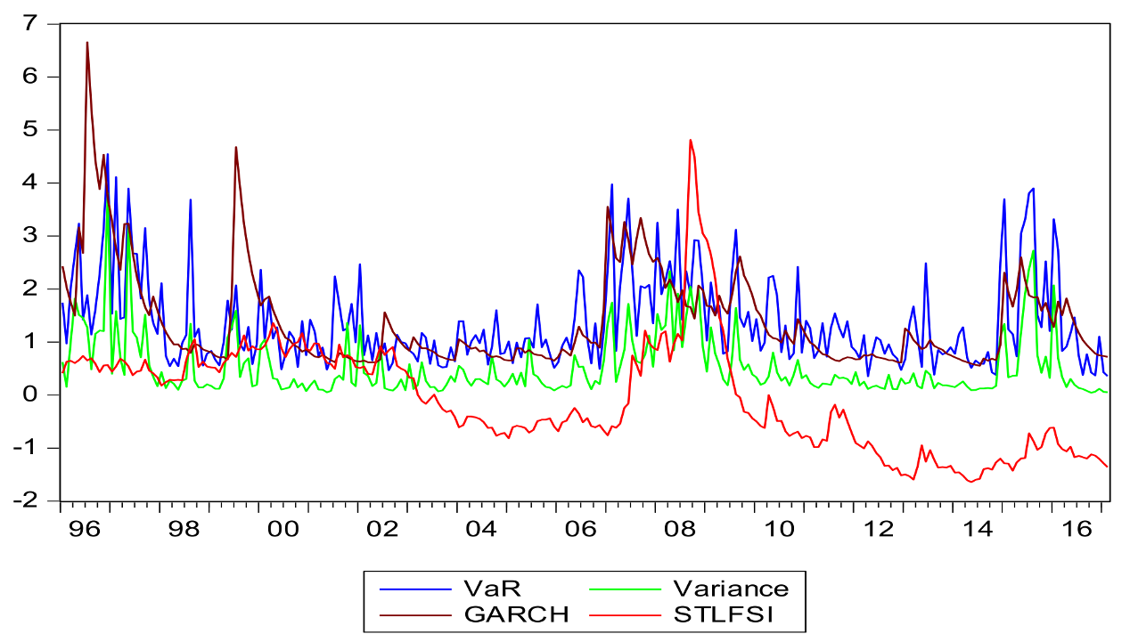
Table 1, which reports summary statistics at the aggregate level of stock returns and extreme values in Chinese stock markets, provides a brief impression of these variables. The monthly return is obtained by taking the log-difference from the end-of-the-month price times 100. This measure closely approximates the average of daily stock returns times 21. The statistics in Table 1 also report the range of monthly returns from −12.26% to 15.15%. The downside risk (VaRt−1), which is obtained from the minimum of the daily stock returns for past 21 trading days times (−1), produces a mean value of 1.369. Other measures of risk expressed by VARIANCE (the unconditional variance), SK (SKEWNESS) and KU (KURTOSIS) (see French et al. 1987; Harvey et al. 2010; Chiang and Li 2013) are derived from 21 trading days for each month of stock returns, and GARCH (conditional variance) is derived by regressing monthly stock returns on a constant term. The time series plotted in Figure 1 reveal that the VaR and GARCH move more closely as compared with the variance, although all the series appear to have some degree of co-movement as reflected in similar turning points and their magnitude of changes. In addition, the chart indicates that GARCH-type variance is smoother as compared with sharply volatile values of VaR. From this perspective, it points out that the underlying risk content has significant business implications in risk management. A point of special note is that the Jarque-Bera (JB) statistics for testing the normality of the return series are found to be highly significant, which leads us to reject the normal distribution hypothesis. This finding is consistent with Gao et al. (2012) and motivates us to use the GED distribution.
Rt = 0.193 + εt
z-stat (1.02)
z-stat (1.51) (2.26) (−1.87) (9.46)
Q(12) is the Ljung -Box statistic to test for correlations of stock return or residual squared up to 12 order lags. The Q(12)-statistic of 19.44 is insignificant at the 5% level. This result suggests the absence of serial correlations of the Chinese stock return. (12) under column R is the Ljung -Box statistic to test for correlations of residual squared from an OLS estimator by regressing stock return on a constant term. The estimated Q-value is 28.07, which is significant at the 5% level based on the Chi-squared test. Checking on the dependency of the level of VARANCE also rejects the null by Q(12).
Table 1 also contains the Q(12), which is the Ljung -Box statistic testing for correlations of stock returns up to 12 order lags. The Q-statistic of 19.44 is insignificant at the 5% level. This result suggests the absence of serial correlations of the Chinese stock return and no lagged term is needed to add to the mean equation. (12) value (28.07) under column R, which is the Ljung -Box statistic to test for correlations of residual squared obtained from an OLS estimator by regressing stock return on a constant term, is significant at the 5% level based on the Chi-squared distribution. This evidence together with the coefficient of the auto correlation function (ACF) of lagged one being significant, indicates that the GED-GARCH(1,1) specification is relevant.12
Next, let us investigate the correlations among the independent variables, which is reported in Table 2. Here we see that the correlation ranges from −0.009 to 0.333 with the highest correlation occurring between domestic downside risk and the U.S. fear index. Due to the existence of this correlation, we shall replace the variable with a neutralized world downside risk in our check for robustness.
6.2. Evidence from the Aggregate Market
Table 3 reports the estimates with various model specifications of China’s aggregate stock market. We manage the heteroscedasticity problem by applying the GED-TARCH(1,1)-M process. To serve as a base for comparison, our estimation begins with a simple model, which only includes the economic fundamentals (Chen et al. 1986) within a TARCH structure. Then we add the conditional volatility and downside risk one at a time to examine the validity of the model and the marginal contribution of the variable using the t-statistic, the Ljung -Box Q statistic and F-values.
Table 3 shows the regression result of Model 1 by regressing the stock return on a constant term plus some fundamental factors commonly used in modeling stock return equations (Chiang et al. 2015; Chiang and Chen 2016a), the investment sentiment (Baker and Wurgler 2006) and liquidity variables (Amihud and Mendelson 1986; Amihud 2002), along with the cross-market contagion effects, U.S. stress index. The testing results show that the coefficient of sentiment variable is positive and statistically significant, indicating that a change toward more optimistic investment sentiment helps to predict a higher stock return. This result is consistent with the finding by Baker and Wurgler (2006, 2007) in the U.S. data, although the components used to measure the sentiment may somehow differ.
One of most important factors that influence business operations and transactions is liquidity. A market or industry suffering from illiquidity usually reflects poorer performance than expected. The illiquidity of stocks is normally accompanied by a lower turnover. To encourage investors to purchase stocks under these conditions, the prevailing stock prices have to fall, causing stock returns to decline. Empirically, the coefficient of the unexpected change in the illiquidity on stock returns, is negative (Amihud 2002; Chiang and Zheng 2015). Because the is, by definition, approximately an inverse of , we anticipate that the coefficient of is positive. The result from Table 3 indicates that the estimated coefficient of is significant and in agreement with our theoretical prediction that the result is positive. This finding matches with the results in the literature (Elyasiani et al. 2000; Chiang and Zheng 2015).13
The estimated results of Model 1 in Table 3 indicate that the coefficient of STLFSIt is negative at the current period but positive in the lagged one period (Bekaert and Harvey 1995). These findings are consistent with the market phenomenon, which holds that when the financial risks rise in the U.S. market, investors in Chinese markets will soon learn of this change through cross-market references of portfolio performance. This information leads to a sell-off of Chinese stocks, which in turn, produces a negative sign for the coefficient of STLFSIt. However, those investors who buy stocks at this high-risk moment are anticipating prices to rise in the near future to compensate for their risk taking, which brings about higher stock prices and, hence, produces a positive coefficient on STLFSIt−1. The evidence in Table 3 indicates that the estimated coefficients for both STLFSIt and STLFSIt−1 are significant at the 5% level.
Despite good results from the economic fundamentals, the above analyses provide no explicit evidence of risk that affects the local stock return. This issue can be investigated using a GED-TARCH(1,1)-M model as shown in Model 2. The results from Table 3 indicate that the estimates of the fundamental factors continue to perform well, and the null hypothesis of the independence of stock-index returns from the conditional standard deviation, , is rejected at the 5% level. The F1(=5.81), the F-statistic for testing incremental efficiency of as an independent variable, is also rejected. Thus, the positive significance of the coefficient of conforms to the risk-return tradeoff hypothesis. In examining the variance equation, we find that all the coefficients in the TARCH(1,1) equation are statistically significant, which indicates that stock return volatilities characterized by a heteroscedastic process display a volatility clustering phenomenon.
As we inspect the time series movements of conditional volatility vis-à-vis the downside risk (GARCH vs. VaR in Figure 1), we see that the GARCH series is smoother than that of VaR, suggesting that these two series may reflect different types of risk. It can be argued that the conditional volatility captures smaller market variations; however, the downside risk reveals a big and negative abrupt change in the stock return. Moreover, the GARCH measure of is derived from the conditional variance using monthly stock return data, while the VaRt−1 is obtained from the minimum value of the past 21 daily returns. Thus, the model that comprises both and VaRt−1 forms a mixed data sampling (or MIDAS) approach and provides more efficient information content in predicting stock returns (Ghysels et al. 2005).
The evidence from Model 3 indicates that in addition to the lagged stress index from the U.S. market, STLFSIt-1, both coefficients, and VaRt−1, are positive and highly significant. The positive risk relation is not only supported by the conventional approach that the risk is generated from a TARCH(1,1) process, but also reveals the significance of downside risk, which features an abrupt, negative plummet on stock returns. From an econometric point of view, one might be concerned with the multicollinearity problem due to the covariance between them over time. However, each risk is derived from different information content, and the significance of each risk measure does not indicate an informational redundancy problem (see Pankratz 1983, p. 203).
The economic interpretations of the positive effect of the lagged downside risk on the stock returns involve rather complex trading behaviors. First, as unexpected negative news hits the market, the positive feedback traders are likely to follow the current market trend of selling off their stocks (Sentana and Wadhwani 1992; Antoniou et al. 2005; Shi et al. 2012), causing a significant drop in prices and a significant loss in stock returns in the current month. Some researchers observe that this big loss tends to generate fear and a pessimistic psychological outlook. Therefore, subsequent portfolio decisions are not necessarily connected to the deterioration of economic fundamentals (Shiller 1981) but rather a demonstration of herding behavior for investors who suppress their private information in making their investment decisions (De Long et al. 1990; Chiang and Zheng 2010).
Unlike positive feedback (noise) traders, contrarian traders consider the current period of dramatically falling market prices as a chance to place new orders. They see the opportunity to profit should a price reversal occur in the near future (De Bondt and Thaler 1985; Sentana and Wadhwani 1992; Govindaraj et al. 2014). A positive sign for VaRt−1 in Table 3 shows this price reversal behavior in the following month, which rewards investors who took the risk.
The high performance of intertemporal downside risk should not be surprising. As implied in the Cornish-Fisher expansion (1937),14 the downside risk contains much of the information of higher moments of stock returns. Thus, using VaR in the test equation not only alleviates the concern of model mis-specification for excluding the higher moments of stock returns in the model but also removes a potential multicollinearity problem.15 We examine the performance of the inclusion of the VaRt−1 in Model 3 by F-statistics. In Model 3, Column F1 tests the incremental effect on the coefficient of VaRt−1 = 0 against Model 2, while Column F2 in Model 3 is the F-statistic for testing both coefficients, and VaRt−1, being zero against Model 1. The calculated F-statistics suggest that the null hypotheses for both cases are rejected. This evidence, along with the Akaike information criterion, concludes that both conditional volatility and downside risk are significant. Moreover, Model 3, by including the downside risk, outperforms the alternatives since the model has a lower Akaike value.
Since the literature contends that it is the risk premium rather than the stock return that needs to be compensated for the risk taken, it is worth testing whether the parametric risk-return relation still holds when stock return is replaced by stock return premium, defined by subtracting one-month risk free rate () from the stock return, that is, . To estimate the model, we replace the dependent variable with the excess stock return, (, which is labelled as Model 4. The estimates of Model 4 are reported in the bottom of Table 3. As shown by the estimated statistics, all the coefficients have their anticipated signs and are statistically significant. The estimated results are comparable to the one we derived from Model 3. In comparison, we find that estimates based on stock return and using excess stock return to serve as a dependent variable do not produce a significant qualitative difference in the estimations. That is, the positive risk-return relation continues to hold true by using the excess stock return as the dependent variable. However, if we judge models by using AIC, Model 3 still comes up with the best performance.
In sum, the estimated results conclude that stock returns can be predicted by using different types of risk: expected market volatility (), downside risk (VaRt) and global market risk (STLFSIt−1) by controlling the fundamental factors. Evidence shows that the GED-TARCH(1,1)-M model is a valid process to describe the monthly trading data in the Chinese stock market. Specifically, the coefficients of the TARCH(1,1) components are statistically significant, indicating that Chinese stock returns, like most other stock return series, display a volatility clustering phenomenon. The asymmetric coefficient is negative, suggesting a significant asymmetric impact on volatility when negative news hits the market. The Q(12) statistics indicate that the return residuals display no serial correlation up to 12-month lags. As we conduct the diagnostic checking on correlations of the residual squares, the Ljund-Box tests from statistics indicate an absence of time series dependency and confirm the GED-TARCH specification for Model 3. Before concluding this section, we should emphasize that the F-test also shows that both the conditional volatility and downside risk are highly significant in predicting stock returns. Therefore, both types of risk should be priced into the stock returns.
6.3. Evidence from Sectoral Markets
Estimates based on the aggregate market provide overall statistics on the behavior of stock returns. However, it contains very little information to advise investors about sectoral performance. To gain some insights on the sectoral characteristics, this section conducts empirical analysis of stock returns over ten sectors in Chinese markets. Using the specification of Model (3) in Table 3, we write the sectoral return equation as follows:
All the variables are defined in the same way as before. However, the subscript i is an index for sectors, where i = 1, 2, …, 10. The specification for Equation (7) follows a similar logic as we provided in the aggregate market.16 The error distribution is comparable to Equation (6) by assuming a generalized error distribution (GED) for each sector. The conditional volatility is measured by the sectoral conditional standard deviation obtained from the GED-TARCH(1,1)-M process as given by Equation (8), and denote the U.S. financial market risk at time t and t − 1. The equation also includes the change in lagged investment sentiment and trading turnovers . The estimations by using GED-TARCH(1,1)-M procedure for sectoral data are reported in Table 4 and Table 5.
As we presented in the case of aggregate market, Table 4 reports the estimates of Equation (7) by excluding , which is equivalent to impose a restriction of in Equation (7). The evidence suggests that estimated results for the sectoral equations continues to have similar qualitative results with respect to the estimated signs and statistical significance. However, there are some minor changes, although all the sectoral coefficients on are positive, only seven out of ten sectors are statistically significant. Specifically, the sectors of Consumer Service, Oil and Gas, and Utilities fail to find support from the data as evidenced by the low t-ratios and F-statistics in Column F1 that reports the F-statistic (1,243) for testing the incremental efficiency for the significance of conditional standard deviation, .
To proceed with our estimation, in Table 5 we add the downside risk to the test equation. The evidence shows that, consistent with the aggregate market, both the coefficients of and display positive signs and are highly significant for all sectors, suggesting that the risk-relation holds true for both volatility-return and downside-risk-return relations. This conclusion can be further supported by checking the F-tests. The F-statistics show not only the incremental variable of being rejected, but also the joint tests for both the coefficients of and being zero are rejected. As shown in Columns F1 and F2, the nulls are uniformly rejected in all sectors with high significant levels. Thus, the sectoral data provide concrete evidence to support that both conditional volatility and market downside risk are priced in the sectoral stock returns.
There are several related points worth noting. First, the magnitude of the coefficients and the associated t-statistics for the are uniformly smaller than that of , suggesting that the downside risk appears to have more sensitive information content to predict stock returns; second, the risk on downside price change differs from the risk of conditional standard deviation. This is because the is derived from the largest price loss in daily trading of the previous month. This price shock tends to create more fear on investors’ decision making; while the is derived from conditional variance based on a TARCH(1,1)-M model using monthly sectoral returns to project future volatility. The type of risk captures a smaller change in volatility, but smoothed risk. Our model thus contains mixed frequency data sampling (MIDAS) for predicting stock returns as advocated by Ghysels et al. (2005). Third, a similar pattern is exhibited in the risk shocks from the external source represented by STLFSIt and STLFSIt−1. The negative coefficient of STLFSIt suggests that all the sectoral returns fall as the Chinese market becomes impinged by a rise of financial stress from the U.S. market. Under this market condition, the investor who places an order for purchasing stocks will expect to have a rise in returns. The test result is expected to find a reward for the risk premium in the subsequent month. However, the evidence shows that only three out of ten sectors are statistically significant for the STLFSIt−1 variable. In fact, the dynamic pricing mechanism from the sectoral reactions is rather complex. The stock returns are tied closely to dynamic price movements, sectoral risk-return rotations, and market expectations, whose results are impacted by the interaction between the positive feedback of traders and rational speculators responding to news (De Long et al. 1990). Fourth, the effect of on stock returns is positive, and estimated coefficients fluctuate widely from the lowest value in the Oil and Gas sector to the highest value in the Basic Material sector. Except for the Oil and Gas sector, the rest of the sectors are statistically significant. Note that the price setting in the Oil and Gas sector is usually tied closely to the pricing mechanism in the world markets. Caporale et al. (2015) find that oil price volatility affects this sector’s stock returns by exhibiting a negative response to oil price uncertainty during periods with supply-side shocks. This external shock may be part of the reason that the parametric relation between stock returns and investment sentiment is insignificant. A general conclusion from the sectoral performance suggests that a higher sentiment as denoted by tends to reflect a more promising business climate and optimistic expectations, attracting investors to long stocks. Fifth, the estimated coefficients on are anticipated to be positive. The estimated coefficients conform to their priori and they are significant for eight out ten sectors. This means that a higher stock return corresponds to a higher liquidity stock. This finding is in line with Amihud (2002) and Chiang and Zheng (2015). It is also interesting to point out that the estimated liquidity coefficient of Industrials sector has the smallest value and the Financial sector turns out to have the largest one. Sixth, with no exception, the lagged error squared components and lagged variance parameters are all statistically significant, indicating that industrial stock returns display a volatility clustering phenomenon. The asymmetric effect, in general, shows a negative sign, with seven out of ten sectors being statistically significant, indicating asymmetric variations of volatility when negative news hits the market.
6.4. Robustness Check
In the above estimations, we are unable to find strong evidence to support the notion by using the U.S. stress index to serve as a global financial market risk. This is probably due to its correlation with the VaRt−1 as we noted in Table 2. Also, a shortcoming by relying on the STLFSIt−1 to serve as the global financial market risk is that all the shocks outside of the U.S. market are excluded from the model and, hence, would lose some information. To address these problems, we use the world downside risk instead. In constructing this series, we find that the information of Chinese VaRt is embodied in the world downside risk, . Thus, without removing the contribution of local country (Chinese) stock index from the world stock index might produce a biased estimator. For this reason, we reconstruct the world VaR series by regressing the on a constant term plus Chinese VaRt.17 The resulting regression residual series gives us the neutralized world VaR series, which is labeled as Thus, and VaRt are independent of each other. To conduct our estimations, we re-write Equation (7) as follows:
The specification of the conditional variance follows the same way as expressed by Equation (8). The estimated results are reported in Table 6. The regression results perform well as reflected in the s, that range from 0.8 to 0.21. Strikingly, all the estimated parameters have their anticipated sign and their corresponding t-ratios are highly significant. The only exceptions are asymmetrical terms in the Banks, Oil and Gas, and Retail sectors, where we fail to find their t-statistics being significant at the 10% level. However, all components of lagged shock squared, and lagged variance are significant, indicating that the GED-TARCH-M model appropriately describes the Chinese sectoral stock return equations and the time series variances are typically displaying a clustering phenomenon. The Ljung -Box Q(12) statistics indicate the absence of serial correlations up to 12 order lags for the return residuals, indicating the adequacy of the model. A similar conclusion can be drawn on testing the correlations of residual squares. As indicated by the reported (12) statistics, none of the residual squared is rejected at the 5% level, indicating that the GED-TARCH(1,1) model is adequate to describe the sectoral model.
Remarkably, this model highlights three different types of risks: and , each of them has its own unique information being used to explain stock returns. To illustrate, represents the risk associated with each sectoral monthly stock return which is modeling from the GED-TARCH process; is the downside risk from the Chinese market; while is the world downside risk. Both downside risks are derived from a minimum return of the past 21 trading days. Thus, the model is featured with a mixed data sampling approach.
In addition to the t-statistics being reported, we also conduct F-tests to distinguish the contribution of each risk, where Column F1 tests the incremental efficiency for the world downside risk, , that is, H0: Column F2 contains the statistics for examining the joint significance of two downside risks, and , that is, H0: Column F3 reports the joint significance of three risks, and , that is, . The testing results clearly indicate that all of the nulls are rejected, confirming the contribution of each risk in predicting stock returns. However, among them, the local downside risk appears to be more influential. In sum, we conclude that the risk-return relation holds true by using all the three different types of risk. It also implies that the conventional study based on either conditional volatility generated from a GARCH model or the local downside risk to test the risk-return relation is likely to commit a specification error.
7. Conclusions
This study conducts empirical analysis on the risk-return relation in Chinese equity markets. Applying the aggregate market and data for ten sectors to test stock return behavior by the TARCH-M procedure, we reach several important empirical conclusions. First, we find significant evidence to support the positive risk-return relation depending on the sources of risk. These findings stem from: (a) evidence that supports the positive risk-return relation when the risk is based on the conditional standard deviation by using the TARCH(1,1)-M procedure to fit the monthly stock returns. (b) We find a positive downside risk-return relation when the downside risk is derived from the greatest loss of daily trading over the past 21 trading days in the Chinese market. (c) The global financial market risk, which is based on the stress index (STLFSI), is priced into the stock returns, although its effect is less profound compared with the previous two types of risk. (d) Our robustness test further confirms that the global downside risk plays a significant role in predicting the Chinese stock return.
Second, evidence supports the notion that the investment sentiment has a predictive power in explaining the stock returns. This holds true for both aggregate data and most of the sectoral analysis. Third, an improvement in liquidity / rise in trading turnover executes predictable power in explaining stock returns. The above testing results hold true in both the aggregate market and sectoral data although some variations occur in the sectoral level.
Fourth, in light of information content of higher moments to explain the risk behavior, we can empirically link the VaR to the corresponding higher moments of stock return distribution by using the Cornish-Fisher expansion (1937). Thus, testing the risk-return relation using the VaR as a regressor turns out to be a more appealing approach, since it not only alleviates the problem of the outlier sensitivity but also helps to capture the higher moments of risk factors.
Fifth, the GED-TARCH(1,1)-M model is an appropriate process to describe the monthly trading data in the Chinese stock market. Specifically, the coefficients on the TARCH(1,1) components are in general statistically significant, indicating that Chinese stock returns display a volatility clustering phenomenon. The threshold coefficient is negative, suggesting a significant asymmetric impact on volatility as negative news hits the market. Finally, the GED distribution can estimate the error series with the leptokurtosis found in the stock return series.
Author Contributions
Thomas Chiang provides an overall structure of the article and offers the theoretical framework, empirical specifications and economic interpretations. Yuanqing Zhang helps to collect and manipulates data as well as performs some statistical computations.
Conflicts of Interest
The authors declare no conflict of interest.
References
- Acharya, Viral V., and Lasse Heje Pedersen. 2005. Asset pricing with liquidity risk. Journal of Financial Economics 77: 375–410. [Google Scholar] [CrossRef]
- Amihud, Yakov. 2002. Illiquidity and stock returns: Cross-section and time-series effects. Journal of Financial Markets 5: 31–56. [Google Scholar] [CrossRef]
- Amihud, Yakov, and Haim Mendelson. 1986. Asset pricing and the bid-ask spread. Journal of Financial Economics 17: 223–49. [Google Scholar] [CrossRef]
- Antoniou, Antonios, Gregory Koutmos, and Andreas Pericli. 2005. Index futures and positive feedback trading: Evidence from major stock exchanges. Journal of Empirical Finance 12: 219–38. [Google Scholar] [CrossRef]
- Bali, Turan G., and Nusret Cakici. 2010. World market risk, country-specific risk and expected returns in international stock markets. Journal of Banking and Finance 34: 1152–65. [Google Scholar] [CrossRef]
- Bali, Turan G., K. Ozgur Demirtas, and Haim Levy. 2009. Is there an intertemporal relation between downside risk and expected returns? Journal of Financial and Quantitative Analysis 44: 883–909. [Google Scholar] [CrossRef]
- Bali, Turan G., and Lin Peng. 2006. Is there a risk-return tradeoff? Evidence from high frequency data. Journal of Applied Econometrics 21: 1169–98. [Google Scholar] [CrossRef]
- Baillie, Richard T., and Ramon P. DeGennaro. 1990. Stock returns and volatility. Journal of Financial and Quantitative Analysis 25: 203–14. [Google Scholar] [CrossRef]
- Baker, Malcolm, and Jeffrey Wurgler. 2006. Investor sentiment and the cross-section of stock returns. Journal of Finance 61: 1645–80. [Google Scholar] [CrossRef]
- Baker, Malcolm, and Jeffrey Wurgler. 2007. Investor sentiment in the stock market. Journal of Economic Perspectives 21: 129–52. [Google Scholar] [CrossRef]
- Batten, Jonathan A., and Peter G. Szilagyi. 2016. The Internationalization of the RMB: New starts, Jumps and tipping points. Emerging Markets Review 28: 221–38. [Google Scholar] [CrossRef]
- Bekaert, Geert, Claude B. Erb, Campbell R. Harvey, and Tadas E. Viskanta. 1998. Distributional characteristics of emerging market returns and asset allocation. Journal of Portfolio Management 24: 102–16. [Google Scholar] [CrossRef]
- Bekaert, Geert, and Campbell R. Harvey. 1995. Time-varying world market integration. Journal of Finance 50: 403–44. [Google Scholar] [CrossRef]
- Bekaert, Geert, Campbell R. Harvey, and Christian Lundblad. 2007. Liquidity and expected returns: Lessons from emerging markets. Review of Financial Studies 20: 1783–831. [Google Scholar] [CrossRef]
- Bollerslev, Tim. 1986. Generalized autoregressive conditional heteroskedasticity. Journal of Econometrics 31: 307–27. [Google Scholar] [CrossRef]
- Bollerslev, Tim. 2010. Glossary to ARCH (GARCH) in Volatility and Time Series Econometrics: Essays in Honor of Robert Engle. Edited by Tim Bollerslev, Jeffrey Russell and Mark Watson. Oxford: Oxford University Press. [Google Scholar]
- Bollerslev, Tim, Ray Y. Chou, and Kenneth F. Kroner. 1992. ARCH modeling in finance: A review of theory and empirical evidence. Journal of Econometrics 52: 5–59. [Google Scholar] [CrossRef]
- Borst, Nicholas. 2017. Connecting China’s Stock Markets to the World. Federal Reserve Bank of San Francisco, January 4. Pacific Exchange Blog. Available online: http://www.frbsf.org/banking/asia-program/pacific-exchange-blog/china-stock-market-connect-shenzhen/ (accessed on 17 March 2018).
- Campbell, John Y., Andrew Wen-Chuan Lo, and Archie Craig MacKinlay. 1997. The Econometrics of Financial Markets. Princeton: Princeton University Press. [Google Scholar]
- Campbell, John Y., and Robert J. Shiller. 1988a. The dividend-price ratio and expectations of future dividends and discount factors. Review of Financial Studies 1: 195–227. [Google Scholar] [CrossRef]
- Campbell, John Y., and Robert J. Shiller. 1988b. Stock prices, earnings, and expected dividends. Journal of Finance 43: 661–76. [Google Scholar] [CrossRef]
- Chen, Nai-Fu, Richard Roll, and Stephen A. Ross. 1986. Economic forces and the stock market. Journal of Business 59: 383–403. [Google Scholar] [CrossRef]
- Chen, Xiaoyu, and Thomas C. Chiang. 2016a. Stock returns and economic forces—An empirical investigation of Chinese markets. Global Finance Journal 30: 45–65. [Google Scholar] [CrossRef]
- Chen, Cathy Yi-Hsuan, and Thomas C. Chiang. 2016b. Empirical analysis of the intertemporal relation between downside risk and expected returns: Evidence from time-varying transition probability models. European Financial Management 22: 749–96. [Google Scholar] [CrossRef]
- Cheng, Ai-Ru, and Mohammad R. Jahan-Parvar. 2014. Risk–return trade-off in the Pacific Basin equity markets. Emerging Markets Review 18: 123–40. [Google Scholar] [CrossRef]
- Chiang, Thomas C., and Jiandong Li. 2013. Modeling Asset Returns with Skewness, Kurtosis, and Outliers. In Handbook of Financial Econometrics and Statistics. Edited by John C. Lee and Cheng-Few Lee. New York: Springer Publishers, chp. 80. [Google Scholar]
- Chiang, Thomas C., and Shuh-Chyi Doong. 2001. Empirical Analysis of Stock Returns and Volatilities: Evidence from Seven Asian Stock Markets Based on TAR-GARCH Model. Review of Quantitative Finance and Accounting 17: 301–18. [Google Scholar] [CrossRef]
- Chiang, Thomas C., Huimin Li, and Dazhi Zheng. 2015b. The Intertemporal Return-Risk Relationship: Evidence from international Markets. Journal of International Financial Markets, Institutions and Money 39: 156–80. [Google Scholar] [CrossRef]
- Chiang, Thomas C., and Xiaoyu Chen. 2016a. Stock returns and economic fundamentals in an emerging market: An empirical investigation of domestic and global market forces. International Review of Economics and Finance 43: 107–20. [Google Scholar] [CrossRef]
- Chiang, Thomas C., and Xiaoyu Chen. 2016b. Empirical Analysis of Dynamic Linkages between China and International Stock Markets. Journal of Mathematical Finance 6: 189–212. [Google Scholar] [CrossRef]
- Chiang, Thomas C., Bang Nam Jeon, and Huimin Li. 2007. Dynamic correlation analysis of financial contagion: Evidence from Asian markets. Journal of International Money and Finance 26: 1206–28. [Google Scholar] [CrossRef]
- Chiang, Thomas C., and Dazhi Zheng. 2010. An empirical analysis of herd behavior in global stock markets. Journal of Banking and Finance 34: 1911–21. [Google Scholar] [CrossRef]
- Chiang, Thomas C., and Dazhi Zheng. 2015. Liquidity and stock returns: Evidence from international markets. Global Finance Journal 27: 73–97. [Google Scholar] [CrossRef]
- Cooper, S. Kerry, John C. Groth, and William E. Avera. 1985. Liquidity, exchange listing and common stock performance. Journal of Economics and Business 37: 19–33. [Google Scholar] [CrossRef]
- Cornish, E.A., and Ronald A. Fisher. 1937. Moments and Cumulants in the Specification of Distribution. Review of the International Statistical Institute 5: 307–20. [Google Scholar] [CrossRef]
- De Bondt, Werner F. M., and Richard Thaler. 1985. Does the stock market overreact? Journal of Finance 40: 793–805. [Google Scholar] [CrossRef]
- De Long, J. Bradford, Andrei Shleifer, Lawrence H. Summers, and Robert J. Waldmann. 1990. Positive feedback investment strategies and destabilizing rational speculation. Journal of Finance 45: 379–95. [Google Scholar] [CrossRef]
- De Santis, Giorgio, and Bruno Gerard. 1997. International asset pricing and portfolio diversification with time-varying risk. Journal of Finance 52: 1881–912. [Google Scholar] [CrossRef]
- Domowitz, Ian, Oliver Hansch, and Xiaoxin Wang. 2005. Liquidity commonality and return co-movement. Journal of Financial Markets 8: 351–76. [Google Scholar] [CrossRef]
- Elyasiani, Elyas, Shmuel Hauser, and Beni Lauterbach. 2000. Market response to liquidity improvements: Evidence from exchange listings. Financial Review 41: 1–14. [Google Scholar] [CrossRef]
- Engle, Robert F. 1982. Autoregressive conditional heteroskedasticity with estimates of variance of United Kingdom inflation. Econometrica 50: 987–1007. [Google Scholar] [CrossRef]
- Engle, Robert F. 1995. ARCH: Selected Readings. Oxford: Oxford University Press, UK. [Google Scholar]
- Engle, Robert F. 2009. Anticipating Correlations: A New Paradigm for Risk Management. Princeton: Princeton University Press USA. [Google Scholar]
- Fama, Eugene F., and Kenneth R. French. 1988. Dividend yields and expected stock returns. Journal of Financial Economics 22: 3–27. [Google Scholar] [CrossRef]
- Fama, Eugene F., and Kenneth R. French. 2015a. A five-factor asset pricing model. Journal of Financial Economics 116: 1–22. [Google Scholar] [CrossRef]
- Fama, Eugene F., and Kenneth R. French. 2015b. Dissecting Anomalies with a Five-Factor Model. Fama-Miller Working Paper. Available online: http://ssrn.com/abstract=2503174 (accessed on 15 December 2017).
- Federal Reserve Bank of St. Louis. 2014. What Is the St. Louis Fed Financial Stress Index? On the Economy. Available online: http://www.stlouisfed.org/on-the-economy/what-is-the-st-louis-fed-financial-stress-index/ (accessed on 30 June 2017).
- Forbes, Kristin J., and Roberto Rigobon. 2002. No contagion, only interdependence: Measuring stock market comovements. Journal of Finance 57: 2223–61. [Google Scholar] [CrossRef]
- French, Kenneth R., G. William Schwert, and Robert F. Stambaugh. 1987. Expected stock returns and volatility. Journal of Financial Economics 19: 3–29. [Google Scholar] [CrossRef]
- Gao, Yan, Chengjun Zhang, and Liyan Zhang. 2012. Comparison of GARCH models on different distributions. Journal of Computers 7: 1967–73. [Google Scholar] [CrossRef]
- Caporale, Guglielmo Maria, Faek Menla Ali, and Nicola Spagnolo. 2015. Oil price uncertainty and sectoral stock returns in China: A time-varying approach. China Economic Review 34: 311–21. [Google Scholar] [CrossRef]
- Ghysels, Eric, Pedro Santa-Clara, and Rossen Valkanov. 2005. There is a risk-return tradeoff after all. Journal of Financial Economics 76: 509–48. [Google Scholar] [CrossRef]
- Glosten, Lawrence R., Ravi Jagannathan, and David E. Runkle. 1993. On the relationship between GARCH and symmetric stable process: Finding the source of fat tails in data. Journal of Finance 48: 1779–802. [Google Scholar] [CrossRef]
- Govindaraj, Suresh, Joshua Livnat, Pavel G. Savor, and Chen Zhao. 2014. Large price changes and subsequent returns. Journal of Investment Management 12: 31–58. [Google Scholar] [CrossRef]
- Harvey, Campbell R., and Akhtar Siddique. 1999. Autoregressive Conditional Skewness. Journal of Financial and Quantitative Analysis 34: 465–87. [Google Scholar] [CrossRef]
- Harvey, Campbell R., John C. Liechty, Merrill W. Liechty, and Peter Muller. 2010. Portfolio selection with higher moments. Quantitative Finance 10: 469–85. [Google Scholar] [CrossRef]
- Karpoff, Jonathan M. 1987. The relation between price changes and trading volume: A survey. Journal of Financial and Quantitative Analysis 22: 109–26. [Google Scholar] [CrossRef]
- Lagarde, Christine. 2015. Press Release: IMF Executive Board Completes the 2015 Review of SDR Valuation. December 1. Available online: http://www.imf.org/en/news/articles/2015/09/14/01/49/pr15543 (accessed on 15 December 2017).
- Lesmond, David A. 2005. Liquidity of emerging markets. Journal of Financial Economics 77: 411–52. [Google Scholar] [CrossRef]
- Lettau, Martin, and Sydney Ludvigson. 2010. Measuring and modeling variation in the risk-return trade-off. In Handbook of Financial Econometrics. Edited by Yacine Aït-Sahalia, Lars Hansen and J. A. Scheinkman. Amsterdam: North Holland. [Google Scholar]
- Li, Hong. 2007. International linkages of the Chinese stock exchanges: A multivariate GARCH analysis. Applied Financial Economics 17: 285–97. [Google Scholar] [CrossRef]
- Merton, Robert C. 1973. An Intertemporal Capital Asset Pricing Model. Econometrica 41: 867–87. [Google Scholar] [CrossRef]
- Merton, Robert C. 1980. On estimating the expected return on the market. Journal of Financial Economics 8: 323–61. [Google Scholar] [CrossRef]
- Nelson, Daniel. 1991. Conditional heteroskedasticity in asset returns: A new approach. Econometrica 59: 347–70. [Google Scholar] [CrossRef]
- Pankratz, Alan. 1983. Forecasting with Univariate Box-Jenkins Models: Concepts and Cases. New York: John Wiley. [Google Scholar]
- Pastor, Ľuboš, and Robert F. Stambaugh. 2003. Liquidity risk and expected stock returns. Journal of Political Economy 111: 642–85. [Google Scholar] [CrossRef]
- Pericoli, Marcello, and Massimo Sbracia. 2003. A primer on financial contagion. Journal of Economic Surveys 17: 571–608. [Google Scholar] [CrossRef]
- Peiro, Amado. 1999. Skewness in financial returns. Journal of Banking and Finance 23: 847–62. [Google Scholar] [CrossRef]
- Rapach, David E., Jack K. Strauss, and Guofu Zhou. 2013. International stock return predictability: What is the role of the United States? Journal of Finance 68: 1633–22. [Google Scholar] [CrossRef]
- Rojas-Suarez, Liliana. 2014. Towards Strong and Stable Capital Markets in Emerging Market Economies. CGD Policy Paper 042. Washington: Center for Global Development, pp. 1–8. [Google Scholar]
- Scott, Robert C., and Philip A. Horvath. 1980. On the direction of preference for moments of higher order than the variance. Journal of Finance 35: 915–19. [Google Scholar] [CrossRef]
- Sentana, Enrique, and Sushil Wadhwani. 1992. Feedback traders and stock return autocorrelations: Evidence from a century of daily data. Economic Journal 102: 415–25. [Google Scholar] [CrossRef]
- Shi, Jian, Thomas C. Chiang, and Xiaoli Liang. 2012. Positive-feedback trading activity and momentum profits. Managerial Finance 38: 508–29. [Google Scholar] [CrossRef]
- Shiller, Robert J. 1981. Do stock prices move too much to be justified by subsequent changes in dividends? American Economic Review 71: 421–36. [Google Scholar]
| 1 | The research along this line has been popularized by the conditional variance (Baillie and DeGennaro 1990) using the generalized autoregressive conditional heteroscedasticity in mean (GARCH-M) model and its extensions to exponential GARCH (Nelson 1991) and threshold GARCH (Glosten et al. 1993). Bollerslev (2010) contains an encyclopedic type reference of ARCH acronyms used in the finance literature. |
| 2 | Chinese RMB constitutes 11% in the IMF’s basket of currencies. |
| 3 | Batten and Szilagyi (2016) provide a timely empirical analysis of the internationalization of the RMB. |
| 4 | Merton’s (1973) original article includes a hedging component that captures the investor’s motive to hedge future investment opportunities. However, a later article by Merton (1980) indicates that the hedging component can be negligible under certain conditions. Thus, the conditional expected excess return can be written as a linear relation of the market’s conditional variance. Some researchers, such as De Santis and Gerard (1997), Bali et al. (2009), Rapach et al. (2013), and Chiang et al. (2015b), prefer to include an additional covariance term between expected excess return and the stated variables to capture other risks besides market risk in their analyses of the CAPM. |
| 5 | In the empirical analysis, a conventional approach that follows an Engle type of model specification and is denoted by , which replaces (Engle 1982, 2009; Bollerslev 1986, 2010). Thus, this paper follows this same approach. |
| 6 | was considered as one of the control variables (Fama and French 1988; Campbell and Shiller 1988a) in the experiment stage. Due to its insignificance, this variable has been excluded. In addition, the higher moments of stock returns were removed from the list of control variables due to the inclusion of VaR, which is implied by the Cornish-Fisher expansion (1937). |
| 7 | Engle (1995, 2009), and Bollerslev (2010) provide different ARCH-type specifications and applications. |
| 8 | A kurtosis above 3 indicates “fat tails”, or leptokurtosis, relative to the normal, or Gaussian, distribution. Platykurtosis refers to a distribution that has a negative excess kurtosis with a relatively flatter peak rather than a normal distribution. |
| 9 | Engle (1995, 2009) and Bollerslev (2010) provide different ARCH-type specifications and applications. |
| 10 | The details of the variable list and the steps to constructing the index are given in the Appendix of National Economic Trends, January 2010; http://research.stlouisfed.org/publications/net/NETJan2010Appendix.pdf. |
| 11 | Baker and Wurgler (2006, 2007) use six different components to construct investment sentiment. Due to different market constraints and availability of data, investment sentiment will be different. |
| 12 | Both the ACF and PACF (partial ACF) for lagged one is 0.189. Comparing this value with the standard error 1/, where T (=observation) = 254, give the t-value = 0.189/0.063 = 3.00, which is significant at the 1% level. |
| 13 | We also estimate the effect by using illiquidity, which is negative and statistically significant. Since the results are similar, we do not report the estimated results here to save space. However, the result is available upon request. |
| 14 | We can use the Cornish-Fisher expansion (Cornish and Fisher 1937)
as a way to relate the -quantile of the probability distribution of stock return at time t, , to its corresponding skewness, and kurtosis, . The equation is: VaRt = 0.62 + 1.199 Vt − 0.387 + 0.069, = 0.90, where |
| 15 | The literature suggests that higher moments are important to explain stock returns (Scott and Horvath 1980; Harvey et al. 2010; Chiang and Li 2013). In an earlier version, we tested the model by including higher moments and the results reveal that the coefficients on the higher moments turn out to be statistically significant. However, the Akaike value turns out to be 5.22, which is higher than that of Model 3. The statistic also shows = 0.16, which is lower than that of Model 3. Therefore, we do not report the equation with higher moments. |
| 16 | Since the evidence shows that using stock return as a dependent variable produces a comparable result as that of excess return, we shall focus on the stock return. |
| 17 | The derivation of follows the same procedure as we derive the Chinese VaR. The is measured by the min of 21 daily stock returns of the world stock price index times (−1). |
Figure 1.
Time series plots of risk measured by VaR, Variance, GARCH and STLFSI.

Table 1.
Summary statistics of market returns, variance, skewness and kurtosis in Chinese markets.
| R | VaR | VARIANCE | GARCH* | SK | KU | MAX | |
|---|---|---|---|---|---|---|---|
| Mean | 0.3110 | 1.3685 | 0.5311 | 1.3966 | −0.05 | 1.3553 | 1.3417 |
| Median | 0.3654 | 1.0974 | 0.3038 | 0.9886 | −0.0569 | 0.8030 | 1.1395 |
| Maximum | 15.1544 | 4.5461 | 3.8087 | 6.6570 | 3.3171 | 13.2937 | 4.1020 |
| Minimum | −12.2664 | 0.3544 | 0.0450 | 0.5515 | −2.3038 | −1.5015 | 0.2958 |
| Std. Dev. | 3.6869 | 0.8477 | 0.5747 | 0.9294 | 0.9106 | 2.1117 | 0.7924 |
| Skewness | 0.1626 | 1.4227 | 2.2623 | 2.0613 | 0.3621 | 2.0003 | 1.3957 |
| Kurtosis | 5.0665 | 4.6027 | 9.4031 | 8.6485 | 3.7430 | 8.6109 | 4.6594 |
| Jonquiere | 46.316 | 112.86 | 650.56 | 517.54 | 11.392 | 502.56 | 111.61 |
| Q(12) | 19.44 | 299.28 | |||||
| (12) | 28.07 | ||||||
| Observations | 254 | 254 | 254 | 254 | 254 | 254 | 254 |
Note: R is the monthly stock market return, VaR is measured by the minimum of 21 daily stock returns times (−1), Variance, SK and KU are higher moments derived from 21 trading days for each month. GARCH* is derived from an asymmetric GARCH(1,1) model by regressing Rt on a constant term. The estimated results are:
Table 2.
Correlation analysis of the independent variables in the stock return equation for Chinese markets.
Table 2.
Correlation analysis of the independent variables in the stock return equation for Chinese markets.
| Correlation | |||||
|---|---|---|---|---|---|
| t-Statistic | |||||
| 1 | |||||
| ----- | |||||
| 0.198 | 1 | ||||
| 2.37 | ----- | ||||
| 0.118 | −0.039 | 1 | |||
| 1.39 | −0.46 | ----- | |||
| 0.160 | −0.009 | 0.022 | 1 | ||
| 1.89 | −0.10 | 0.26 | ----- | ||
| 0.143 | 0.333 | −0.027 | 0.022 | 1 | |
| 1.69 | 4.13 | −0.31 | 0.26 | ----- | |
Note: is the conditional standard deviation, VaRt-1 is the downside risk, is the change in investors’ sentiment, is the change in trading volume turnover, and STLFSIt-1 is the St. Louis Fed stress index. The subscript (t − 1) refers to a one-period lag of time t. The number in the first row is the correlation coefficient, the second row is the t-statistic of the estimated correlation coefficient.
Table 3.
Estimates of aggregate stock returns on conditional volatility, downside risk, investment sentiment, trading turnover, U.S. market stress based on a GED-TGARCH-M model.
Table 3.
Estimates of aggregate stock returns on conditional volatility, downside risk, investment sentiment, trading turnover, U.S. market stress based on a GED-TGARCH-M model.
| Model | STLFSIt | STLFSIt−1 | Akaike | F1 | F2 | ||||||||||||
|---|---|---|---|---|---|---|---|---|---|---|---|---|---|---|---|---|---|
| 1 | 0.320 | 88.842 | 2.101 | −1.085 | 1.139 | 1.417 | 0.250 | −0.282 | 0.858 | 11.22 | 11.22 | 5.30 | 0.02 | ||||
| 4.85 | 9.04 | 10.99 | −4.78 | 5.03 | 1.09 | 1.24 | −1.37 | 8.01 | 0.51 | 0.51 | |||||||
| 2 | −1.288 | 0.378 | 80.283 | 1.657 | −0.926 | 0.913 | 2.386 | 0.325 | −0.265 | 0.751 | 9.51 | 9.51 | 5.31 | 5.81 | 0.05 | ||
| −1.86 | 2.41 | 5.28 | 7.83 | −2.03 | 2.11 | 2.25 | 1.50 | −1.29 | 8.88 | 0.60 | 0.60 | 0.02 | |||||
| 3 | −1.347 | 1.145 | 2.367 | 70.535 | 1.577 | −0.460 | 0.706 | 1.543 | 0.378 | −0.286 | 0.752 | 13.54 | 13.54 | 5.07 | 609. | 304.7 | 0.18 |
| −1.56 | 4.46 | 24.69 | 7.30 | 7.55 | −2.32 | 3.34 | 2.56 | 3.38 | −3.01 | 23.70 | 0.33 | 0.33 | 0.00 | 0.00 | |||
| 4 | 3.174 | 0.199 | 2.831 | 264.47 | 8.216 | −5.707 | 5.249 | 9.186 | 0.858 | −0.494 | 0.668 | 10.78 | 10.78 | 7.20 | 7.88 | 0.16 | |
| 2.86 | 1.84 | 8.69 | 13.49 | 12.33 | −5.14 | 4.91 | 0.94 | 1.32 | −0.85 | 4.23 | 0.55 | 0.55 | 0.00 |
Note: The dependent variable is the market stock return at time t, Rt, for Models 1–3. The dependent variable in Model 4 is the excess stock return, , t-statistics are below the estimated coefficient. The critical values of 1%, 5% and 10% levels are 2.576, 1.96, and 1.645, respectively. is the Ljung -Box statistic to test for correlations of residual (squared) up to 12 order lags. The numbers below the Q-statistics are the p-values. Akaike is the Akaike Information Criterion. F1 is the F(1,243)-statistic for testing the incremental efficiency for the downside risk (VaR), while F2 is the F(2,242) statistics for testing the joint hypothesis of the coefficients of and being zero. The numbers below F1 and F2 are the p-values. Since the null is strongly rejected as indicated by the p-values, the evidence suggests that positive risk-return relations hold true in the Chinese stock markets.
Table 4.
Estimates of stock returns on downside risk, U.S. market stress, sentiment, and liquidity with a GED-TARCH-M process.
Table 4.
Estimates of stock returns on downside risk, U.S. market stress, sentiment, and liquidity with a GED-TARCH-M process.
| Sectors | STLFSIt | STLFSIt−1 | Akaike | F1 | |||||||||
|---|---|---|---|---|---|---|---|---|---|---|---|---|---|
| Basic_M | −0.560 | 0.229 | 99.651 | 1.803 | −1.608 | 1.743 | 0.705 | 0.311 | −0.299 | 0.875 | 5.62 | 2.96 | 0.04 |
| −0.97 | 1.72 | 4.43 | 9.38 | −2.69 | 2.92 | 0.80 | 1.54 | −1.49 | 10.30 | 0.09 | |||
| Banks | −12.016 | 1.450 | 36.127 | 0.863 | −1.049 | 0.543 | 27.258 | 0.130 | 0.276 | 0.512 | 5.71 | 23.98 | 0.06 |
| −9.82 | 15.49 | 2.20 | 4.12 | −3.08 | 1.52 | 3.17 | 3.34 | 3.17 | 9.23 | 0.00 | |||
| Cons_Svs | −4.142 | 0.900 | 45.328 | 0.755 | −1.619 | 1.566 | 15.577 | 0.477 | −0.172 | 0.290 | 5.61 | 1.78 | 0.04 |
| −1.15 | 1.34 | 5.77 | 5.97 | −5.09 | 4.88 | 2.85 | 1.18 | −0.88 | 2.77 | 0.18 | |||
| Financial | −2.459 | 0.535 | 83.595 | 1.046 | −1.396 | 1.147 | 6.086 | 0.428 | −0.017 | 0.475 | 5.56 | 6.82 | 0.08 |
| −2.86 | 2.61 | 5.38 | 4.09 | −4.62 | 3.41 | 2.81 | 2.12 | −0.10 | 6.88 | 0.01 | |||
| Ind.Gs&S | −0.991 | 0.305 | 37.848 | 0.844 | −1.047 | 0.722 | 3.699 | 0.451 | −0.263 | 0.665 | 5.57 | 4.63 | 0.02 |
| −1.56 | 2.15 | 3.38 | 6.38 | −3.80 | 2.67 | 1.93 | 1.67 | −1.22 | 8.78 | 0.03 | |||
| Industrials | −1.522 | 0.322 | 64.621 | 0.543 | −1.213 | 0.777 | 3.533 | 0.440 | −0.420 | 0.697 | 5.76 | 4.35 | 0.02 |
| −2.20 | 2.09 | 3.72 | 1.65 | −2.11 | 1.35 | 1.80 | 1.65 | −1.57 | 6.35 | 0.04 | |||
| Oil&Gas | −0.671 | 0.159 | 55.241 | 2.597 | −1.175 | 1.386 | 3.061 | 0.751 | −0.811 | 0.840 | 5.49 | 2.50 | 0.02 |
| −1.19 | 1.58 | 8.78 | 52.34 | −4.13 | 4.81 | 1.68 | 1.27 | −1.25 | 24.92 | 0.11 | |||
| Real Estate | −18.948 | 3.420 | 59.969 | 0.901 | −1.695 | 1.812 | 21.987 | 0.006 | 0.040 | 0.267 | 5.89 | 13.38 | 0.00 |
| −4.14 | 3.66 | 2.52 | 3.95 | −3.24 | 3.42 | 4.62 | 0.92 | 2.07 | 3.75 | 0.00 | |||
| Retail | −1.511 | 0.453 | 119.98 | 0.959 | −0.520 | 0.403 | 1.243 | 0.329 | −0.205 | 0.713 | 5.67 | 2.90 | 0.03 |
| −1.56 | 1.70 | 3.24 | 1.48 | −0.62 | 1.01 | 1.63 | 3.04 | −1.84 | 9.04 | 0.09 | |||
| Utilities | 0.592 | 0.003 | 83.777 | 0.314 | −2.074 | 2.153 | 0.835 | 0.187 | −0.320 | 0.937 | 5.73 | 0.00 | 0.02 |
| 1.19 | 0.02 | 2.66 | 0.34 | −4.89 | 5.04 | 3.83 | 8.51 | −10.64 | 96.25 | 0.98 |
Note: The dependent variable is market/sectoral stock returns. The first row reports the estimated coefficients, the second row reports the t-statistics, the critical values of the 1%, 5% and 10% levels are 2.576, 1.96, and 1.645, respectively. “Akaike” is the Akaike Information Criterion. F1 is the F-statistic (1,243) for testing the incremental efficiency for the significance of conditional standard deviation, . The number below the F-value is the p-value. Rejection of the null supports the portfolio return and market risk tradeoff.
Table 5.
Estimates of stock returns on downside risk, U.S. market stress, sentiment, and liquidity with a GED-TARCH-M process.
Table 5.
Estimates of stock returns on downside risk, U.S. market stress, sentiment, and liquidity with a GED-TARCH-M process.
| Sectors | STLFSIt | STLFSIt−1 | Q(12) | Akaike | F1 | F2 | ||||||||||
|---|---|---|---|---|---|---|---|---|---|---|---|---|---|---|---|---|
| Basic_M | −2.900 | 1.343 | 2.163 | 122.219 | 2.007 | −1.069 | 1.685 | 1.691 | 0.161 | −0.128 | 0.830 | 9.58 | 5.51 | 108.89 | 57.29 | 0.17 |
| −1.39 | 2.74 | 10.44 | 6.76 | 8.90 | −2.99 | 4.13 | 2.02 | 2.08 | −1.78 | 17.31 | 0.65 | 0.00 | 0.00 | |||
| Banks | −6.284 | 0.956 | 1.554 | 103.642 | 0.846 | −0.171 | −0.341 | 27.65 | 0.300 | 0.350 | 0.473 | 17.41 | 5.62 | 219.64 | 120.2 | 0.05 |
| −2.21 | 2.82 | 14.82 | 9.68 | 4.56 | −0.43 | −0.85 | 3.14 | 2.08 | 1.46 | 11.18 | 0.14 | 0.00 | 0.00 | |||
| Cons_Svs | −0.088 | 0.806 | 1.969 | 111.103 | 1.355 | 0.366 | −0.190 | 1.733 | 0.422 | −0.293 | 0.601 | 13.48 | 5.36 | 56.33 | 28.23 | 0.19 |
| −0.10 | 2.79 | 7.51 | 3.36 | 2.55 | 0.50 | −0.26 | 3.04 | 2.88 | −2.00 | 7.52 | 0.26 | 0.00 | 0.00 | |||
| Financial | −0.193 | 0.589 | 1.639 | 53.415 | 2.075 | −1.323 | 1.299 | 2.168 | 0.542 | −0.188 | 0.602 | 13.03 | 5.44 | 92.62 | 46.93 | 0.14 |
| −0.33 | 3.59 | 9.62 | 3.01 | 8.40 | −3.00 | 2.94 | 2.13 | 2.46 | −0.97 | 10.16 | 0.38 | 0.00 | 0.00 | |||
| Ind.Gs&S | −1.383 | 0.940 | 2.032 | 42.573 | 0.539 | −0.562 | 0.549 | 2.723 | 0.624 | −0.391 | 0.577 | 11.94 | 5.42 | 219.32 | 157.9 | 0.13 |
| −2.26 | 6.65 | 14.81 | 2.35 | 2.61 | −1.49 | 1.49 | 2.97 | 3.80 | −2.50 | 9.71 | 0.48 | 0.00 | 0.00 | |||
| Industrials | −1.971 | 0.945 | 2.129 | 67.970 | 0.490 | −1.064 | 0.461 | 1.548 | 0.280 | −0.261 | 0.796 | 13.22 | 5.63 | 114.06 | 57.16 | 0.09 |
| −1.97 | 3.38 | 10.68 | 3.17 | 1.56 | −1.95 | 0.83 | 2.77 | 2.20 | −1.91 | 19.57 | 0.35 | 0.00 | 0.00 | |||
| Oil&Gas | 0.110 | 0.721 | 2.176 | 15.497 | 1.678 | −0.258 | 0.022 | 2.157 | 0.481 | −0.268 | 0.500 | 14.11 | 5.20 | 72.75 | 36.71 | 0.13 |
| 0.12 | 2.37 | 8.53 | 0.53 | 3.47 | −0.41 | 0.03 | 3.59 | 2.86 | −1.36 | 4.62 | 0.29 | 0.00 | 0.00 | |||
| Real Estate | −4.328 | 1.468 | 1.818 | 78.107 | 0.704 | −0.831 | 0.739 | 1.796 | 0.137 | −0.111 | 0.831 | 10.41 | 5.71 | 53.87 | 28.10 | 0.10 |
| −1.77 | 2.60 | 7.34 | 2.76 | 1.60 | −1.69 | 1.27 | 1.98 | 2.05 | −1.66 | 18.55 | 0.58 | 0.00 | 0.00 | |||
| Retail | −1.035 | 0.770 | 1.443 | 109.601 | 1.014 | −0.728 | 0.931 | 1.363 | 0.288 | −0.191 | 0.727 | 12.42 | 5.62 | 19.24 | 9.95 | 0.08 |
| −0.86 | 2.18 | 4.39 | 3.11 | 1.85 | −0.87 | 1.15 | 1.64 | 2.71 | −1.80 | 10.03 | 0.41 | 0.00 | 0.00 | |||
| Utilities | 0.730 | 0.674 | 1.704 | 98.223 | 1.295 | −2.371 | 2.255 | 1.573 | 0.107 | −0.289 | 0.955 | 11.00 | 5.71 | 51.39 | 25.75 | 0.02 |
| 1.75 | 4.49 | 7.17 | 2.28 | 1.66 | −5.43 | 4.25 | 4.37 | 4.11 | −9.48 | 47.62 | 0.53 | 0.00 | 0.00 |
Note: The dependent variable is sectoral stock returns. The first row reports the estimated coefficients, the second row reports the t-statistics, the critical values of the 1%, 5% and 10% levels are 2.576, 1.96, and 1.645, respectively. is the Ljung -Box statistic for testing residual correlations up to 12 order lags. The number below the Q-statistic is the p-value. Akaike is the Akaike Information Criterion. F1 is the F(1,242)-statistic for testing the incremental efficiency for the downside risk (VaR), while F2 is the F(2,242) statistic for testing the joint hypothesis of the coefficients of and being zero. The numbers below F1 and F2 are the p-values.
Table 6.
Estimates of stock returns on local downside risk, world downside risk, sentiment, and liquidity with a GED-TARCH-M process.
Table 6.
Estimates of stock returns on local downside risk, world downside risk, sentiment, and liquidity with a GED-TARCH-M process.
| Market | Q(12) | (12) | Akaike | F1 | F2 | F3 | |||||||||||
|---|---|---|---|---|---|---|---|---|---|---|---|---|---|---|---|---|---|
| Market | −0.989 | 1.133 | 2.413 | 0.347 | 57.873 | 1.897 | 1.263 | 0.335 | −0.296 | 0.799 | 12.07 | 4.95 | 5.07 | 20.19 | 227.71 | 163.61 | 0.21 |
| −1.57 | 7.43 | 20.96 | 4.49 | 4.85 | 9.51 | 3.01 | 6.66 | −5.42 | 35.59 | 0.44 | 0.96 | 0.00 | 0.00 | 0.00 | |||
| Basic_M | −0.417 | 1.015 | 2.720 | 0.428 | 98.723 | 1.659 | 1.573 | 0.216 | −0.231 | 0.805 | 12.40 | 15.39 | 5.49 | 6.81 | 67.26 | 44.95 | 0.19 |
| −0.27 | 2.41 | 11.51 | 2.61 | 3.84 | 4.71 | 2.40 | 2.03 | −2.09 | 16.93 | 0.41 | 0.22 | 0.01 | 0.00 | 0.00 | |||
| Banks | −3.870 | 1.235 | 1.375 | 0.332 | 130.02 | 1.090 | 8.316 | 0.187 | −0.037 | 0.488 | 9.36 | 9.68 | 5.51 | 36.14 | 86.17 | 77.74 | 0.14 |
| −3.28 | 5.57 | 11.64 | 6.01 | 8.91 | 4.22 | 3.95 | 3.34 | −0.51 | 9.60 | 0.67 | 0.64 | 0.00 | 0.00 | 0.00 | |||
| Cons_Svs | −7.279 | 2.863 | 2.259 | 0.241 | 96.614 | 1.632 | 2.895 | 0.154 | −0.176 | 0.745 | 12.51 | 10.77 | 5.33 | 4.27 | 63.37 | 55.39 | 0.28 |
| −2.81 | 3.88 | 11.50 | 2.07 | 4.22 | 5.25 | 3.34 | 2.84 | −2.87 | 15.05 | 0.25 | 0.55 | 0.04 | 0.00 | 0.00 | |||
| Financial | −7.564 | 1.531 | 1.138 | 0.643 | 136.25 | 0.799 | 22.51 | 0.342 | −0.229 | 0.327 | 8.02 | 12.81 | 5.54 | 139.4 | 121.49 | 98.43 | 0.17 |
| −2.61 | 3.12 | 14.78 | 11.81 | 13.87 | 4.99 | 4.20 | 2.35 | −2.18 | 12.21 | 0.78 | 0.38 | 0.00 | 0.00 | 0.00 | |||
| Ind.Gs&S | −2.021 | 0.830 | 2.006 | 0.365 | 20.689 | 0.631 | 9.450 | 0.932 | −0.881 | 0.462 | 18.05 | 18.82 | 5.57 | 19.64 | 1071.5 | 717.23 | 0.13 |
| −1.24 | 2.52 | 46.29 | 4.43 | 2.48 | 9.64 | 3.21 | 1.87 | −1.90 | 11.22 | 0.11 | 0.09 | 0.00 | 0.00 | 0.00 | |||
| Industrials | −0.260 | 0.360 | 1.587 | 0.711 | 71.024 | 0.512 | 14.52 | 0.653 | −0.863 | 0.529 | 12.38 | 8.21 | 5.87 | 100.8 | 78.84 | 54.53 | 0.10 |
| −0.48 | 5.59 | −10.56 | −10.04 | 6.71 | 2.28 | 2.25 | 2.87 | −2.71 | 7.69 | 0.42 | 0.77 | 0.00 | 0.00 | 0.00 | |||
| Oil&Gas | −2.108 | 1.030 | 2.059 | 0.115 | 70.619 | 2.208 | 2.797 | 0.156 | −0.036 | 0.788 | 12.26 | 3.72 | 5.26 | 3.93 | 197.28 | 133.8 | 0.15 |
| −1.18 | 2.31 | 19.28 | 1.98 | 6.29 | 16.46 | 2.55 | 1.90 | −0.75 | 17.86 | 0.43 | 0.99 | 0.00 | 0.00 | 0.00 | |||
| Real Est. | −2.957 | 1.165 | 2.103 | 0.585 | 98.427 | 0.537 | 0.949 | 0.160 | −0.117 | 0.884 | 11.50 | 5.86 | 5.74 | 24.75 | 93.19 | 63.57 | 0.10 |
| −2.07 | 4.09 | 11.93 | 4.97 | 6.00 | 1.92 | 1.56 | 3.06 | −2.05 | 38.40 | 0.48 | 0.92 | 0.00 | 0.00 | 0.00 | |||
| Retail | −0.946 | 0.762 | 1.517 | 0.352 | 93.754 | 0.939 | 0.725 | 0.132 | −0.069 | 0.866 | 12.92 | 8.84 | 5.69 | 2.69 | 12.38 | 8.42 | 0.08 |
| −0.63 | 1.94 | 4.78 | 1.64 | 2.46 | 1.67 | 1.15 | 1.97 | −0.91 | 14.32 | 0.38 | 0.72 | 0.10 | 0.00 | 0.00 | |||
| Utilities | −3.160 | 1.153 | 1.830 | 0.253 | 85.819 | 1.415 | 1.684 | 0.104 | −0.117 | 0.887 | 13.93 | 6.07 | 5.28 | 9.00 | 268.40 | 179.93 | 0.10 |
| −2.14 | 3.90 | 22.20 | 3.00 | 8.02 | 11.16 | 3.36 | 3.02 | −2.84 | 88.17 | 0.31 | 0.91 | 0.00 | 0.00 | 0.00 |
Note: The dependent variable is the market/sectoral stock returns. The first row reports the estimated coefficients, the second row reports the t-statistics. The critical values of the 1%, 5% and 10% levels are 2.576, 1.96, and 1.645, respectively. ( is the Ljung Box statistic for testing residual (squared) correlations up to 12 order lags. The numbers below the Q(12)-statistic F1, F2 and F3 are the F-statistics. Q-statistic for Cons.Svs is the result from adding AR(4,6) in the model. Akaike is the Akaike Information Criterion. F1 is the F(1,236)-statistic for testing the incremental efficiency for the world downside risk () being zero; F2 is the F(2,236) statistic for testing the joint hypothesis of the coefficients of and being zero; F3 is the F(3,236)-statistic for testing the joint hypothesis of the coefficients of and being zero.
© 2018 by the authors. Licensee MDPI, Basel, Switzerland. This article is an open access article distributed under the terms and conditions of the Creative Commons Attribution (CC BY) license (http://creativecommons.org/licenses/by/4.0/).
Share and Cite
MDPI and ACS Style
Chiang, T.C.; Zhang, Y. An Empirical Investigation of Risk-Return Relations in Chinese Equity Markets: Evidence from Aggregate and Sectoral Data. Int. J. Financial Stud. 2018, 6, 35. https://doi.org/10.3390/ijfs6020035
AMA Style
Chiang TC, Zhang Y. An Empirical Investigation of Risk-Return Relations in Chinese Equity Markets: Evidence from Aggregate and Sectoral Data. International Journal of Financial Studies. 2018; 6(2):35. https://doi.org/10.3390/ijfs6020035
Chicago/Turabian StyleChiang, Thomas C., and Yuanqing Zhang. 2018. "An Empirical Investigation of Risk-Return Relations in Chinese Equity Markets: Evidence from Aggregate and Sectoral Data" International Journal of Financial Studies 6, no. 2: 35. https://doi.org/10.3390/ijfs6020035
Note that from the first issue of 2016, this journal uses article numbers instead of page numbers. See further details here.