An End-to-End Lightweight Multi-Scale CNN for the Classification of Lung and Colon Cancer with XAI Integration

Abstract

To effectively treat lung and colon cancer and save lives, early and accurate identification is essential. Conventional diagnosis takes a long time and requires the manual expertise of radiologists. The rising number of new cancer cases makes it challenging to process massive volumes of data quickly. Different machine learning approaches to the classification and detection of lung and colon cancer have been proposed by multiple research studies. However, when it comes to self-learning classification and detection tasks, deep learning (DL) excels. This paper suggests a novel DL convolutional neural network (CNN) model for detecting lung and colon cancer. The proposed model is lightweight and multi-scale since it uses only 1.1 million parameters, making it appropriate for real-time applications as it provides an end-to-end solution. By incorporating features extracted at multiple scales, the model can effectively capture both local and global patterns within the input data. The explainability tools such as gradient-weighted class activation mapping and Shapley additive explanation can identify potential problems by highlighting the specific input data areas that have an impact on the model’s choice. The experimental findings demonstrate that for lung and colon cancer detection, the proposed model was outperformed by the competition and accuracy rates of 99.20% have been achieved for multi-class (containing five classes) predictions.

1. Introduction

Cancer is a health condition that is characterized by the unregulated growth of abnormal cells that can develop in any tissue or organ inside the body. The World Health Organization says that it was the second most common cause of death in the world in 2020, with about 10 million deaths [1]. Compared to other cancer types, colorectal cancer accounts for 1.80 million new cases and 783 thousand fatalities, whereas lung cancer contributes to 1.76 million new cases and 1.76 million fatalities. The two varieties of lung cancer that spread and grow quickly are small-cell lung cancer (SCLC) and non-small-cell lung cancer (NSCLC) [2,3]. Cells with neuroendocrine characteristics cause SCLC, which accounts for 15% of all instances of lung cancer and remains a hazardous form of the disease. The three pathologic types of NSCLC, including immense cell carcinoma, adenocarcinoma, and squamous cell carcinoma, account for 85% of all cases [4]. The most common cause of death is colorectal cancer, which accounts for 10.7% of all instances [1].

To examine the therapy possibilities in the early stages of the disease, a more precise diagnosis of various cancer subtypes is required. For lung cancer, radiography, computed tomography (CT) imaging, flexible sigmoidoscopy, and CT colonoscopy are among the non-invasive diagnostic techniques [4]. Histopathology is one simple test that can be required to effectively diagnose the disease and improve the quality of treatment. However, non-invasive techniques may not always produce effective classifications of these cancers. Additionally, pathologists may grow exhausted from manually grading histological images. Additionally, expert pathologists are required for the precise classification of lung and colon cancer (LCC) subtypes; manual grading may be prone to mistakes. To lessen the workload on pathologists, automated image processing techniques for LCC subtype screening are necessary [5].

There are a lot of different methods for diagnosing cancer symptoms. The amount of data kept in archives is increasing daily because of technical improvements [5]. The rising accessibility of healthcare data offers researchers opportunities to enhance current methods for more in-depth clinical analysis [6]. Artificial intelligence (AI) techniques like machine learning (ML) and DL are the foundation of automatic diagnosis approaches. Researchers have solved numerous health challenges and applications using a variety of traditional machine learning techniques [7,8]. The traditional method for utilizing ML to retrieve and categorize photos in the medical area is solely dependent on manually constructed features created through the feature engineering process. All kinds of characteristics must be used to automatically classify LCC. Filtering and segmentation algorithms can retrieve intensity values and texture descriptors, which are examples of low-level features that are important aspects of an image. Additionally, low-level characteristics can be extracted automatically from LCC images using feature extraction methods, including Haralick characteristics and local binary patterns (LBPs). They function as a base for representations of higher-level features [9].

The characteristics of the surrounding tissue, as well as the tumor’s location, size, and shape, are important classification criteria for LCC. Both low-level and high-level features must be considered for automatic tumor categorization to be accurate and reliable. The basic characteristics of images are captured by low-level features, while high-level features offer general and meaningful data [10]. Thus, due to its capacity to deal with these drawbacks and its powerful discrimination capabilities, DL has gained popularity for use in medical testing [11]. These features can be automatically extracted using DL techniques, and they are necessary to organize treatments and make correct diagnoses. Combining these features is required to obtain high accuracy. Convolutional neural network (CNN) is a well-known DL architecture that is frequently employed in this context [12]. Through their numerous deep layers, CNN models may identify high-level features in raw data. In this manner, CNNs can successfully analyze complicated and challenging data. These models have an increasing number of parameters, along with substantial complexity [13]. The complexity and depth of the CNN architecture are what make the models so successful.

Based on the CNN model, explainable artificial intelligence (XAI) is a useful tool in the medical industry that increases the transparency of automatically generated prediction models. It speeds up the creation of predictive models, utilizing expertise in the field and helping to produce results that are understandable to humans [14,15]. There are several ways to show the most active areas and to make a model more explicable. A few examples of these techniques include utilizing XAI algorithms, Shapley Additive Explanation (SHAP), and gradient-weighted class activation mapping (Grad-CAM) [16] for the model’s explanatory categorization [17].

It is not easy to process LCC datasets using conventional methods as there are various challenges, such as the following:

▪

Most of these techniques have substantial computing costs and require a lot of labeled training data.

▪

Overfitting can happen when the model works well with training data but poorly with new, untested data.

▪

Risk of poor performance brought on by inaccurate or biased training data.

▪

DL models’ decision-making process is not explainable.

To avoid overfitting or inaccurate diagnosis, it is essential to use DL models that have been thoroughly tested and proven on large, diverse datasets. It is also critical to use techniques like cross-validation (CV) to account for any possible biases in the data used for training to guarantee the model’s wider applicability. The overall objective of the proposed method is to be improved by offering precise and early diagnoses that allow for quick and efficient treatment. This paper focuses on categorizing lung and colon cancer subtypes using histopathological images from a dataset named LC25000, which is publicly available on Kaggle. There are a total of five classes in the dataset, which are benign lung tissue, lung adenocarcinomas, lung squamous cell carcinoma, benign colon tissue, and colon adenocarcinomas.

Compared to DL models, the suggested model is less complex and very lightweight, with only eight layers, which makes it appropriate for real-time applications and mobile applications. The originality of the proposed work can be summed up as follows:

• A novel lightweight multi-scale (LW-MS) end-to-end CNN model for the identification of LCC is introduced. The proposed model has 1.1 million trainable parameters and is superior to other models in this field, which need deeper layers to achieve acceptable detection accuracy. This reduces processing time and model complexity, making the system suitable for real-time applications.
• To increase the accuracy and efficiency of multi-class predictions, predictions from multiple layers are concatenated to produce a range of feature maps that function at different resolutions.
• XAI techniques have been integrated into the proposed LW-MS CNN model with its performance metrics analysis. This aspect has frequently been neglected in prior studies.
• A web application system has been developed with the purpose of aiding pathologists and doctors in the diagnosis of histological pictures and offering substantiation for their scientific findings.

The remainder of the article is organized as follows. Section 2 includes a review of the literature on the most current DL advancements related to LCC detection. Section 3 discusses the proposed method in detail. Section 4 presents and thoroughly discusses the experimental setup and achieved results. Section 5 summarizes the proposed model’s findings and discusses the model. Finally, Section 6 concludes the research and suggests potential future research directions.

2. Related Works

To classify images of lung tissues from histopathology, a computer-aided system (CAD) method was developed by Nishio et al. [18]. They extracted visual characteristics from two datasets using homology-based processing of images (HI) and traditional texture analysis (TA), and then they assessed the effectiveness of eight ML algorithms. In both datasets, the HI-equipped CAD system outperformed the TA system. They concluded that for CAD systems, HI was significantly more advantageous than TA and that this could lead to the development of an accurate CAD system. Similarly, Mangal et al. [19] developed a CAD system by looking at digital pathology images and using CNN to identify lung and colon cancer. In comparison to deep CNN models that employ TL trained on a similar collection and classical ML models, their experimental results on the LC25000 showed a decent accuracy of 96.61% for the colon and 97.89% for the lung, which were acquired by the CNN using the most recent feature descriptions. Shandilya et al. [20] have created a CAD technique to categorize lung tissue histology pictures. They employed a dataset of histological pictures of lung tissue that was made publicly available for the development and validation of CAD. Multi-scale processing was used to extract image features. Seven CNN models that had been hyper-tuned before were used in a comparative analysis to predict lung cancer, with ResNet101 achieving the greatest overall accuracy at 98.67%. Masud et al. [21] used DL on histopathology pictures to present a categorization system for five different types of lung and colon tissues. First, image sharpening was applied to pathological example images. A CNN model that was manually tweaked was trained using these features. This model’s accuracy performance was reported to be 96.33%.

Similarly, Hatuwal et al. [22] stated a CNN-based technique for classifying histological images to diagnose cancer. They built and trained a neural network with a specific shape. The accuracy in training and validation were reported to be 96.11% and 97.20%, respectively. Similar to this, three CNN models were introduced by Tasnim et al. [23] to assess colon cell imaging data. To calculate the learning rate, the models were developed and put to the test at various epochs. It was demonstrated that the maximum pooling layer has an accuracy of 97.49%, while the average pooling layer has an accuracy of 95.48%. MobileNetV2 outperforms the previous two versions, with a 99.67% accuracy rate and a 1.24% loss rate. However, Sikder et al. [24] have suggested a novel technique for separating, recognizing, classifying, and spotting various malignant cell types in RGB and MRI images. They merged a CNN model with a SegNet method that employs anatomical changes that were better than the regular SegNet model to shorten training times and enhance segmentation results. The proposed method identified cancer cells from several cancer datasets with an average accuracy rate of 93%. They were able to overcome the drawbacks of using different cancer detection methods for MRI and histopathology data.

A CNN model for predicting colon cancer developed by Qasim et al. [25] is notable for its speed and accuracy, with few parameters. They used two separate strategies in their model and then 256 feature maps were created by each. By increasing the number of features at different levels, they were able to increase the accuracy and sensitivity. The same dataset was used to develop and train the VGG16, which was used to evaluate the effectiveness of the suggested strategy. The proposed model’s achieved accuracy is 99.6%, while the VGG16’s is 96.2%. The results suggest that it was effective in detecting colon cancer. To classify different forms of lung and colon cancer, Talukder et al. [1] have introduced a combination of ensemble attribute-obtaining techniques. Ensemble learning for image filtering and the deep feature extraction method were combined. The proposed hybrid model reportedly had a 99.05% accuracy rate in identifying the possibility of cancer. Hanan et al. [26] have presented the Marine Predator Algorithm with DL (MPADL-LC3) method for classifying lung and colon cancer. This method leveraged MobileNet to generate feature vectors and used CLAHE-based contrast enhancement as a preprocessing step. They introduced MPA as a hyper-parameter optimizer, and a deep belief network was applied for classification. With a maximum accuracy of 99.27%, the comparison research emphasized the improved results of the MPADL-LC3 approach.

Attallah et al. [27] have created a lightweight DL method. To achieve feature reduction and provide a more comprehensive representation of the data, the architecture uses various transformation techniques. In that sense, the SqueezeNet, ShuffleNet, and MobileNet algorithms are fed with HSI. Thus, the features extracted from the model are decreased by using PCA models and the fast Walsh–Hadamard transform (FHWT). It obtained 99.6% accuracy. Al-Jabbar et al. [28] have suggested a method that combines ANN with fusion features and CNN models. The ANN achieved an accuracy of 99.64% with VGG-19 fusion features and handcrafted features. By analyzing the LC2500 dataset, Sameh et al. [29] have built a unique deep network for LCC fine-tuning using pre-trained ResNet101. Hyper-parameter optimizations were used to make these improvements. They obtained 99.84%, 99.85%, 99.84%, 99.96%, and 99.94% scores for their model’s precision, recall, F1-score, specificity, and accuracy, respectively. Imran et al. [30] have proposed a deep CNN model for the automated detection and characterization of colon cancer, in which textured images are trained in high resolution without being converted into low-resolution images by changing the classification of binary data in the resultant activation layer to the sigmoid function. They achieved 99.80% recall, 99.87% F1-score, 99.80% accuracy, and 100% precision. Two methods were presented by Kumar et al. [3]. Six approaches for extracting handcrafted aspects based on color, texture, shape, and structure are provided in one method. They also employed seven frameworks for DL that extract features from deep data from histopathology pictures, with the idea of transfer learning. However, compared to manually created features, deep CNN network features show a considerable boost in classifier performance. The LCC tissue was recognized by the Random Forest classifier, with DenseNet-121 retrieving deep features with an accuracy and recall of 98.60%, precision of 98.63%, F1 score of 0.985, and receiver operating characteristic curve (ROC)—area under the ROC Curve (AUC) of 1.

Even though numerous research works show the outstanding accuracy in limited-class and binary classification scenarios, their performance steadily deteriorates as the number of classes rises. This phenomenon results from the growing difficulty of differentiating between many diseases with precisely various characteristics. This restriction makes the models less useful in actual clinical settings where patients may present with a range of lung diseases. Consequently, to perform a multi-class classification of lung and colon diseases with high accuracy and confidence for real-life scenarios, a customized and reliable deep learning framework is needed. In this study, a LW-MS CNN with 1.1 million parameters has been proposed to produce a more promising outcome than the state-of-the-art (SOTA) models. Nevertheless, Grad-CAM and SHAP have been used for showing the effectiveness of the model by detecting ROI despite all the challenges. Also, to the best of the authors’ knowledge, only a small number of studies have so far demonstrated these explainable AI methods to show interpretability.

3. Proposed Method

This section discusses the proposed method in depth. This section also covers the datasets used in this research. Furthermore, a detailed discussion of each step of the suggested process, including how the images have been pre-processed, and clear insight into the lightweight multi-scale convolutional cancer network (LW-MS-CCN) is included. Moreover, this section discusses the explainable AI methods used in this paper. Figure 1 outlines the suggested framework for detecting LCC from histopathological images.

3.1. Dataset Description

The publicly accessible dataset LC25000 [31] was used for this research. For this dataset, a Leica microscope LM190 HD camera coupled to an Olympus BX41 microscope was used to collect each subtype of LCC, taking 250 color photos, 1250 total photos in total, and without any data augmentation. Next, the 250 samples for every subtype of cancer were multiplied via augmentation techniques, like left and right rotations and horizontal and vertical flips, to create 5000 images. Consequently, upon data augmentation, there were already 25,000 typical histopathology photos in the dataset, with 10,000 images showing colon cancer and 15,000 showing lung cancer. Three cell labels, including adenocarcinomas, squamous cell carcinoma, and benign tissue, were present in the lung cancer dataset. Adenocarcinomas and benign tissue are two examples of the two cell labels found in the colon cancer dataset. Prior to applying data augmentation, the photos were resized from their original 1024 × 768 resolution to 768 × 768.

Images of lung, colon, and both types of cancer were used in this work. Hence, there were 25,000 photos in total—10,000 for colon tissue and 15,000 for lung tissue for both the colon and the lung. The distribution of the cancerous dataset is presented in

Table 1. Number of images in each class.

Classes	No. of Images
Benign lung tissue	5000
Lung adenocarcinomas	5000
Lung squamous cell carcinoma	5000
Benign colon tissue	5000
Colon adenocarcinomas	5000

.

3.2. Data Pre-Processing

For medical image analysis, image preprocessing is essential, since the classification performance varies depending on how well the image has been preprocessed [32]. To train the model, the input image was reduced to 180 × 180. To work with image intensity values, the resized image was converted into bgr2rgb, and then the images were converted into a NumPy array. After that, a technique called scaling was used to normalize image intensity values between 0 and 1. By dividing the image array by 255, the image was scaled to reduce computing complexity. Finally, the image label has been added, which is a crucial step because it enables us to recognize cancerous images.

3.3. Lightweight Multi-Scale Convolution Cancer Network

A compact, straightforward, and yet efficient model has been created. The LW-MS-CCN has a single input layer that is 180 × 180 × 3 in size. Globalmaxpooling2D was utilized after each convolutional layer to pick out the most crucial details from each feature map, make them smaller, combine them, and then use this combined information to understand the image better. Globalmaxpooling2D obtains critical values using the max operation. One method to address overfitting difficulties is the dropout layer [33]. Figure 2 shows the design of the LW-MS-CCN model proposed in this method. The dataset was divided according to an 80/20 rule: 80% of the data were used for training and 20% were utilized for testing. There are 12 convolution layers in the backbone CNN. To avoid high dimensionality, using more filters in higher layers was avoided when designing the custom CNN. It can automatically extract characteristics from input images without requiring human interaction [34]. The model’s capacity to extract discriminative features from data by utilizing a lightweight CNN as its foundation, convolutional layers as the head for feature extraction across many scales, and filter size optimizations histopathological pictures was improved.

Several convolutional layers are stacked and added to the top of the backbone model to form the CNN head. These convolutional layers are added to the model head, allowing the architecture to be tailored for the extraction of features at various scales. Deeper layers in the CNN head learn more complicated and abstract characteristics, whereas the CNN layers closer to the input learn low-level features like edges and textures. This is essential for classification, since unpredictability in the picture can have unusual appearances. Through multi-scale feature mapping, the model’s overall accuracy in classification is improved, making it more resilient and able to recognize unpredictability of different sizes.

The network starts with “Layer 1”, which consists of two convolutional layers, both using a 3 × 3 kernel size and a 180 × 180 input size. The first layer has 7 filters, and the second layer has 9 filters. After each convolutional layer, a max pool layer with a 2 × 2 kernel size is applied. In this research, filters of 2 × 2 size were used to apply max pooling. The maximum value is chosen for each window as the pooling window advances over the feature maps. The spatial dimensions of the feature map are cut in half by utilizing a pooling window of 2 × 2 and a stride of 2 [35]. In order to achieve translation invariance and resilience against minute spatial alterations, max pooling is successful in capturing the most important characteristics within local areas. Next, “Layer 2” has two convolutional layers, where the input size is reduced to 90 × 90. The first layer in this layer has 16 filters, and the second layer has 32 filters. Again, after each convolutional layer, a max pool layer is used. “Layer 3” further reduces the input size to 45 × 45 and contains two convolutional layers with 256 filters each. After each convolution, max pool is applied. “Layer 4” consists of three convolutional layers, which results in a reduction in the input size to 22 × 22. The initial two layers are equipped with 32 filters each, while the third layer is equipped with 64 filters. “Layer 5” consists of two convolutional layers with an input size of 11 × 11. The starting layer is equipped with 64 filters, while the subsequent layer also employs 64 filters. Finally, “Layer 6” includes two convolutional layers with an input size of 5 × 5. Both layers have 128 filters. Max pool is used after each convolution. In summary, the custom CNN architecture is built with a consistent pattern of 3 × 3 convolutional layers, followed by 2 × 2 max pool layers, progressively reducing the input size and increasing the number of filters in deeper layers.

This design aims to capture and learn hierarchical features from the input image data, ultimately leading to more accurate predictions for the given classification task. From

Table 2. An overview of the proposed model that includes the number of parameters and information about each layer.

Layer (Type)	Output Shape	Params	Connected to
Input 1	(None, 180, 180, 3)	0
conv2d	(None, 180, 180, 7)	196	Input 1
conv2d_1	(None, 180, 180, 9)	576	conv2d
max_pooling2d	(None, 90, 90, 9)	0	conv2d_1
conv2d_2	(None, 90, 90, 16)	1312	max_pooling2d
conv2d_3	(None, 90, 90, 32)	4640	conv2d_2
max_pooling2d_1	(None, 45, 45, 32)	0	conv2d_3
conv2d_4	(None, 45, 45, 32)	9248	max_pooling2d_1
conv2d_5	(None, 45, 45, 64)	18,496	conv2d_4
max_pooling2d_2	(None, 22, 22, 64)	0	conv2d_5
conv2d_6	(None, 22, 22, 64)	36,928	max_pooling2d_2
conv2d_7	(None, 22, 22, 64)	36,928	conv2d_6
max_pooling2d_3	(None, 11, 11, 64)	0	conv2d_7
conv2d_8	(None, 11, 11, 64)	36,928	max_pooling2d_3
conv2d_9	(None, 11, 11, 128)	73,856	conv2d_8
max_pooling2d_4	(None, 5, 5, 128)	0	conv2d_9
conv2d_10	(None, 5, 5, 128)	147,584	max_pooling2d_4
conv2d_11	(None, 5, 5, 128)	147,584	conv2d_10
max_pooling2d_5	(None, 2, 2, 128)	0	conv2d_11
conv2d_11	(None, 2, 2, 32)	32,896	max_pooling2d_5
conv2d_12	(None, 2, 2, 64)	18,496	conv2d_11
conv2d_13	(None, 2, 2, 128)	73,856	conv2d_12
concatenate	(None, 2, 2, 224)	0	conv2d_13, conv2d_12, conv2d_11
flatten	(None, 896)	0	concatenate
dense	(None, 512)	459,264	flatten
dropout	(None, 512)	0	dense
dense_1	(None, 5)	2565	dropout
Total params	11,05,353
Trainable params	11,05,353
Non-trainable params	0

and Figure 2, it can be seen that the max_pooling2d_5 (last max pooling layer of CNN block) is connected to conv2d_11 (head of multi-scale CNN). conv2d_11, conv2d_12, and conv2d_13 are all the layers connected together in a concatenate layer, which enables the network to simultaneously use data from several scales. After that, flatten layer is used to convert all the features into 1D vector. Then, as the flattened characteristics move through dense layers, high-level abstraction and pattern detection are made easier. After using dropout regularization to reduce overfitting, a final dense layer with softmax activation is used to produce class probabilities. The model can learn rich representations of the input data across multiple levels of abstraction according to the multi-scale CNN design, which efficiently combines features from different scales.

Table 2 provides an overview of the proposed LW-MS-CCN model architecture, detailing the number of parameters and information about each layer. The model comprises a series of convolutional and pooling layers, culminating in fully connected layers. The total number of parameters is 1,105,353, all of which are trainable.

Table 3. Hyper-parameters of the proposed LW-MS-CCN model.

Parameters	Value
Loss function	Sparse-categorical-cross-entropy
Initial learning rate	0.0001
No. of epochs	100
Batch size	16
Shuffle	Every epoch

outlines the hyper-parameters utilized in training the LW-MS-CCN model. Selecting hyper-parameters for a CNN involves a combination of domain knowledge, empirical experimentation, and sometimes trial and error. For classification problems with multiple classes, a categorical cross-entropy technique is commonly used. The ‘sparse’ variant is used when the labels are integers rather than one-hot encoded. A small learning rate, like 0.0001, is often chosen to ensure stable convergence. Learning rates are often tuned through experimentation, and techniques like learning rate schedules or adaptive learning rate methods may be employed. Too few epochs may result in under fitting, while too many may lead to overfitting. The optimal number of epochs is determined through training on a validation set, and techniques like early stopping may be used to prevent overfitting. Smaller batch sizes often lead to faster convergence, and larger batch sizes can provide a regularizing effect and speed up training. Batch sizes are selected based on computational constraints and experimentation to find a balance between speed and model performance. Shuffling the training data every epoch helps prevent the model from memorizing the order of examples and improves generalization. These hyper-parameters contribute to the effective learning and convergence of the LW-MS-CCN model, ensuring its successful application to the given task.

3.4. XAI

XAI describes the ability of an AI system to provide understandable and interpretable explanations for its decisions and actions, enhancing transparency and trustworthiness [36]. XAI in medical imaging helps bridge the gap between AI technology and medical practitioners, making AI-assisted diagnosis and treatment more trustworthy, understandable, and reliable. In XAI, the “black-box” concept refers to AI models that make decisions without providing clear or understandable reasons, while the “white-box” concept pertains to AI models that are transparent and provide interpretable explanations for their decisions, making their internal workings accessible and comprehensible to humans [37]. The XAI methods that have been used in this paper are explained below.

3.4.1. Grad-CAM

Grad-CAM is a visualization method used in DL for understanding model decisions, especially in computer vision tasks. The approach utilizes the gradients of the target class with respect to the final convolutional layer to generate a heatmap. The final convolutional layers are chosen for their balance between spatial information and high-level semantics, allowing for the visualization of class-specific details in the input image [17,38].

By emphasizing regions where the model focuses its attention to create distinctive patterns, Grad-CAM leverages the rich information in the final layer. The algorithm computes gradients of the class score with respect to feature maps, performs weighted combinations, and generates a heatmap, effectively highlighting key areas in the input image that contribute to the target class prediction [39].

$$L_c^{CAM}=\sum _i \sum _j{w}_c^k{A}_k^{ij}$$

(1)

where $L_c^{CAM}$ is the localization map for class $c$ in GradCAM. $w_c^k$ is the weight associated with the $k$-th feature map for class $c$. $A_k^{ij}$ is the activation of the $k$-th feature map at a spatial location $\left(i,j\right)$. $\sum _i\sum _j$ is double summation over spatial dimensions. This equation represents the GradCAM formulation for obtaining a class-specific localization map by combining the feature weights $\left(w_c^k\right)$ with the activations $\left(A_k^{ij}\right)$ from different spatial locations.

3.4.2. SHAP Visualization

SHAP aims to explain predictions in ML models by calculating the contribution of each feature to a given prediction instance. It utilizes coalitional game theory to derive Shapley values, representing the fair contributions of individual features to the prediction. In this technique, the feature values of a data instance act as players in a coalition, and Shapley values help distribute the prediction fairly among these features. Players can be single feature values or collections of feature values, such as super-pixels in images. SHAP introduces a novel approach by presenting Shapley values as a linear model and linking them with the values of local interpretable model-agnostic explanations. This additive feature attribution model provides a comprehensive explanation of the prediction [16].

$$g\left(z^{\prime }\right)={\varphi }_0+{\sum }_{j=1}^M{\varphi }_{\mathrm{j}}{z}_j^{\prime }$$

(2)

where $g$ is the explanation model, $z^{\prime }\in \{\mathrm{0,1}{\}}^M$ is the coalition vector, M is the maximum coalition size, and ${\varphi }_j\in \mathbb{R}$ is the feature attribution for a feature j; the Shapley values. The expression is a linear combination of input features $z_j^{\prime }$ weighted by coefficients ${\varphi }_j$, and the result is adjusted by an intercept term ${\varphi }_0$.

4. Result Analysis

In this section, all the experimental setups and results of this research will be described in detail.

4.1. Experimental Setup

The experimental setup of the proposed system is described in this subsection.

Table 4. System specifications of the proposed framework.

Features	Specifications
Programming Language	Python (version-3.10.12)
Environment	Google Colab
Backend	Keras with TensorFlow
Disk Space	78.2 GB
GPU RAM	15 GB
GPU	Nvidia Tesla T4
System RAM	12.72 GB
Operating System	windows 11
Input	LCC Images
Input Size	180 × 180
Web Development Tool	Gradio Library

accommodates the system specifications upon which the proposed work has been based. All coding operations have been performed in Google Colab, which has a backend of Keras with TensorFlow, and the disk space for it is 78.2 GB. The GPU used was a Nvidia Tesla T4 with a RAM size of 15 GB. In this study, the operating system was Windows 11, and for visualization in web environments, Gradio Library was used.

4.2. Performance Metrics of the Proposed Framework

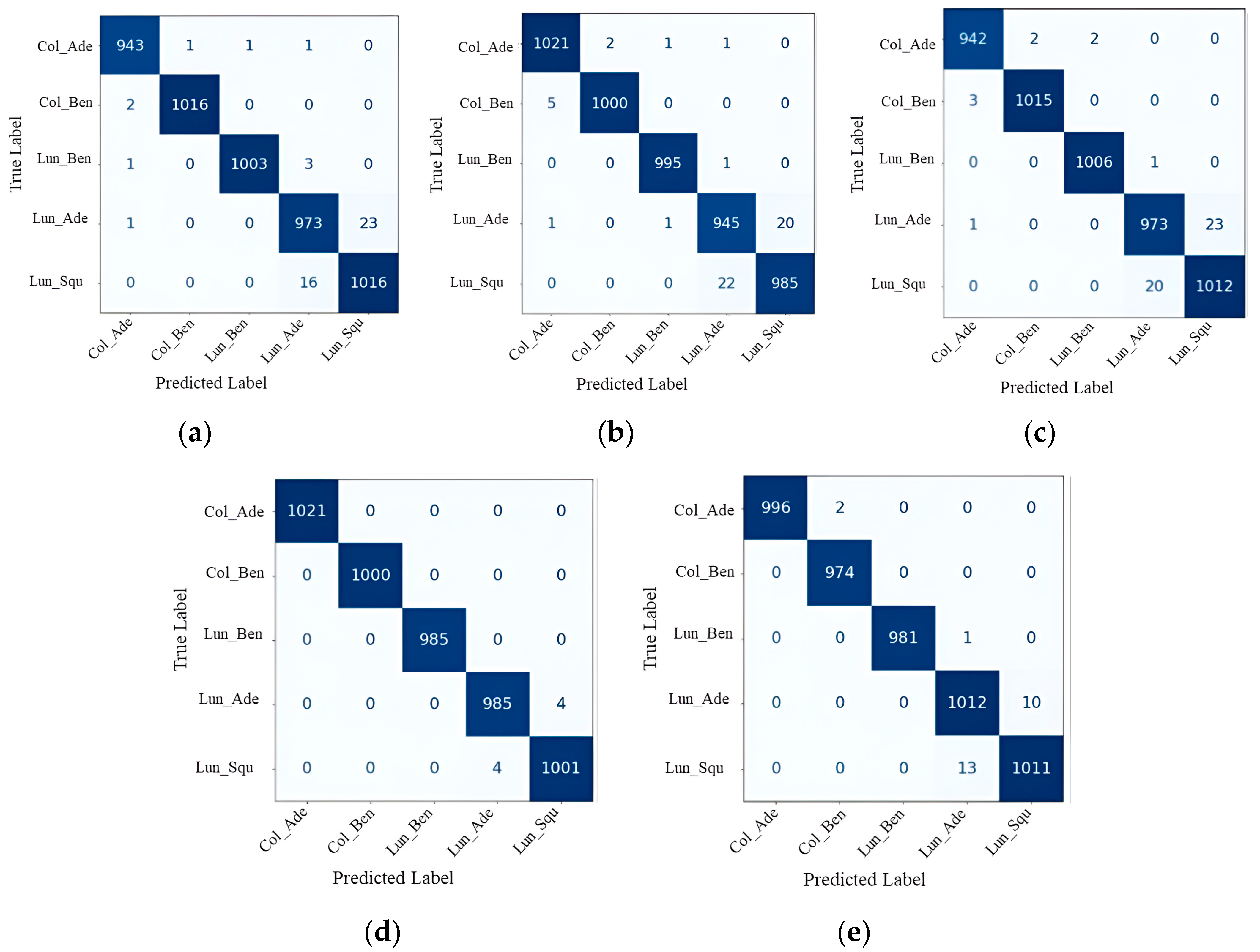
The confusion matrix is a technique for assessing how well ML categorization works. The terms TP (true positive) and TN (true negative) accurately reflect expected positive values. TP represents a correctly predicted positive value, FP (false positive) represents a false positive value, and FN (false negative) represents a false negative value. They are highly helpful in determining the ROC curve, F1-score, accuracy, recall, and precision.

The most obvious performance statistic is accuracy, which is directly proportional to the number of properly predicted observations over the total number of observations [40,41].

$$\mathrm{A}\mathrm{c}\mathrm{c}\mathrm{u}\mathrm{r}\mathrm{a}\mathrm{c}\mathrm{y}=\frac{\mathrm{T}\mathrm{P}+\mathrm{T}\mathrm{N}}{\mathrm{T}\mathrm{P}+\mathrm{F}\mathrm{P}+\mathrm{T}\mathrm{N}+\mathrm{F}\mathrm{N}}$$

(3)

Precision is defined as the proportion of accurately anticipated positive values to all positively predicted values. It is shown as follows:

$$\mathrm{P}\mathrm{r}\mathrm{e}\mathrm{c}\mathrm{i}\mathrm{s}\mathrm{i}\mathrm{o}\mathrm{n}=\frac{\mathrm{T}\mathrm{P}}{\mathrm{T}\mathrm{P}+\mathrm{F}\mathrm{P}}$$

(4)

Recall [42] is defined as the ratio of all the actual values to the values that were positively predicted and successfully made. It is demonstrated as follows:

$$\mathrm{R}\mathrm{e}\mathrm{c}\mathrm{a}\mathrm{l}\mathrm{l}=\frac{\mathrm{T}\mathrm{P}}{\mathrm{T}\mathrm{P}+\mathrm{F}\mathrm{N}}$$

(5)

The harmonic mean of a classification problem’s precision and recall scores is known as the F1-score [43]. The F1-score is shown as follows:

$$\mathrm{F}1-\mathrm{s}\mathrm{c}\mathrm{o}\mathrm{r}\mathrm{e}=\frac{2\times \mathrm{p}\mathrm{r}\mathrm{e}\mathrm{c}\mathrm{i}\mathrm{s}\mathrm{i}\mathrm{o}\mathrm{n}\times \mathrm{r}\mathrm{e}\mathrm{c}\mathrm{a}\mathrm{l}\mathrm{l}}{\mathrm{p}\mathrm{r}\mathrm{e}\mathrm{c}\mathrm{i}\mathrm{s}\mathrm{i}\mathrm{o}\mathrm{n}\times \mathrm{r}\mathrm{e}\mathrm{c}\mathrm{a}\mathrm{l}\mathrm{l}}$$

(6)

ROC curves are two-dimensional graphs that are used for evaluating and understanding classifier performance [44]. Classifiers are graded and chosen according to particular user requirements, which are often associated with changeable error costs and accuracy expectations [45,46]. The sensitivity or specificity interchanges in a classifier for all possible classification thresholds are displayed in detail on the ROC graphs. The AUC measures the degree of distinction, whereas the ROC is a likelihood curve. It demonstrates a model’s ability to discriminate across various groups. Plotting the false positive rate on the x-axis corresponds to the genuine positive rate on the y-axis. An AUC near 1 suggests that the expected model performs well in terms of class label separability, whereas an AUC near 0 denotes a poorly anticipated model. Actually, the word “lousy” means that the effect is being reflected [47]. It is a method for demonstrating the effectiveness of a classification [48]. The best classifiers are those with greater ROC curves [49].

$$\mathrm{A}\mathrm{U}\mathrm{C}=\frac{1}{2}\left(\frac{\mathrm{T}\mathrm{P}}{\mathrm{T}\mathrm{P}+\mathrm{F}\mathrm{N}}+\frac{\mathrm{T}\mathrm{N}}{\mathrm{T}\mathrm{N}+\mathrm{F}\mathrm{P}}\right)$$

(7)

Specificity is a metric that evaluates the ability of a model to correctly detect true negatives within each available class. The mathematical expression can be expressed as follows [48].

$$\mathrm{S}\mathrm{p}\mathrm{e}\mathrm{c}\mathrm{i}\mathrm{f}\mathrm{i}\mathrm{c}\mathrm{i}\mathrm{t}\mathrm{y}=\frac{\mathrm{T}\mathrm{N}}{\mathrm{T}\mathrm{N}+\mathrm{F}\mathrm{P}}$$

(8)

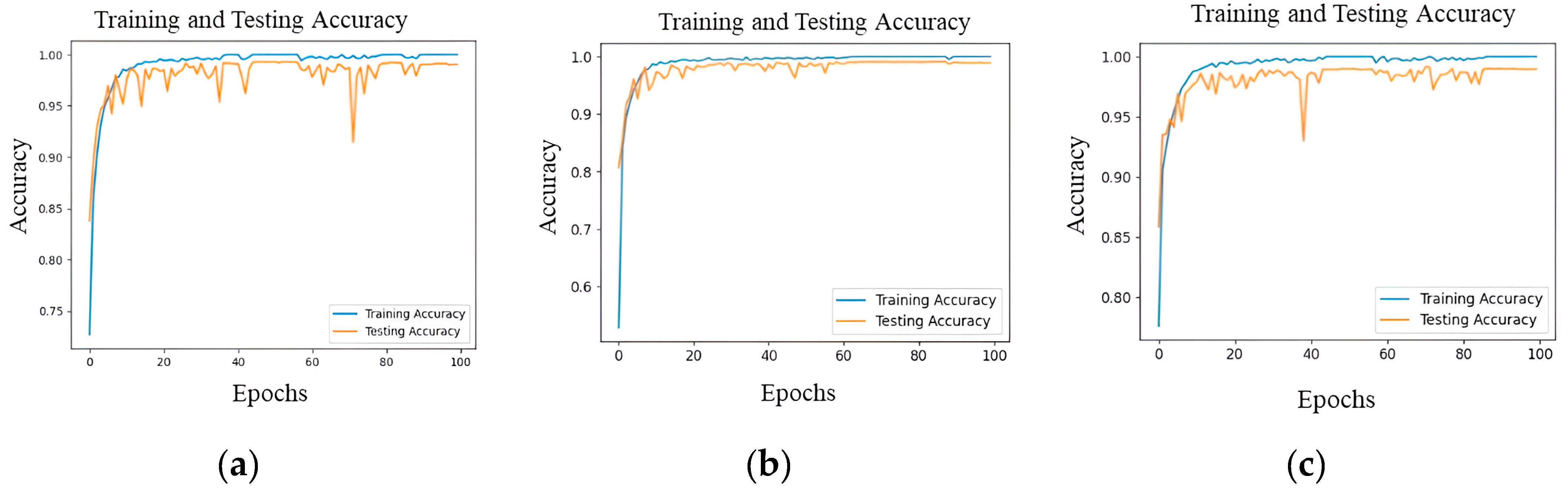
The XAI performance metrics include normalized root mean square error (nRMSE), which is a standardized form of the root mean square error (RMSE). The metric calculates the mean size of the discrepancies between projected and actual values, which is then adjusted based on the data’s range. It offers a standardized way to quantify errors, allowing for meaningful comparisons across diverse datasets. The structural similarity index (SSIM) is a perceptual model that takes into account brightness, contrast, and structure. The normalized index quantifies the degree of structural similarity between two images. The values go from −1 to 1, with a value of 1 denoting photo that are identical. The multi-scale structural similarity index (MS-SSIM) is an extension of SSIM that takes into account changes in image resolution by using multiple scales. It offers a more adaptable assessment of structural similarity by taking into account variations in image viewing conditions. Using the k-fold CV technique, k, smaller sets are created from a training set. The plan is to train a model on each of the k “folds” and then validate it using the remaining data. Using k-fold CV, the average of the values computed in the loop is then included as an evaluation metric. For LCC detection experiments, k-fold CV with a value of k = 5 has been used. Five distinct folds are created from the dataset, and each is used as a testing component while the dataset is being folded. The dataset is divided into 80% for training and the remaining 20% for testing in a k-fold.

4.3. Performance Evaluations

In this section, the performance of the proposed model on the LC25000 dataset is demonstrated. The performance is evaluated with different performance metrics as well as by using XAI like Grad-CAM and SHAP to evaluate the proposed model based on which portion of the image the decision is made on and what predicting the class is.

Performance Evaluation of Lung and Colon Cancer

Table 5. Performance metrics analysis of LW-MS-CCN model for each class of the LCC dataset.

Fold Number	Class	Accuracy (%)	Precision (%)	Recall (%)	F1-Score (%)	Specificity (%)	AUC
Fold = 1	Col_Ade	99.92	99.71	99.90	99.80	99.37	100
	Col_Ben	99.92	99.90	99.70	99.80	99.68	100
	Lun_Ben	99.98	100	99.90	99.95	99.57	100
	Lun_Ade	99.24	97.69	98.48	98.09	100	100
	Lun_Squ	99.26	98.50	97.81	98.15	100	100
	Average	99.66	99.16	99.16	98.16	99.72	100
Fold = 2	Col_Ade	99.80	99.42	99.61	99.51	99.40	100
	Col_Ben	99.86	99.80	99.50	99.65	99.81	100
	Lun_Ben	99.94	99.80	99.90	99.85	99.71	100
	Lun_Ade	99.08	97.52	97.72	97.62	97.89	100
	Lun_Squ	99.16	98.01	97.82	97.91	99.61	100
	Average	99.57	98.91	98.91	98.91	99.68	100
Fold = 3	Col_Ade	99.84	99.58	99.58	99.58	99.68	100
	Col_Ben	99.90	99.80	99.71	99.75	99.57	100
	Lun_Ben	99.94	99.80	99.90	99.85	99.79	100
	Lun_Ade	99.10	97.89	97.59	97.74	100	100
	Lun_Squ	99.14	97.78	98.06	97.92	100	100
	Average	99.58	98.97	98.97	98.97	99.81	100
Fold = 4	Col_Ade	99.82	100	99.80	99.80	100	100
	Col_Ben	99.94	99.70	99.60	99.80	100	100
	Lun_Ben	99.98	99.90	99.90	99.95	100	100
	Lun_Ade	99.37	98.69	99.50	98.09	99.60	100
	Lun_Squ	99.45	98.89	98.89	98.15	100	100
	Average	99.71	99.39	99.54	99.16	99.92	100
Fold = 5	Col_Ade	99.75	99.42	99.58	99.40	99.80	100
	Col_Ben	99.80	99.75	99.71	99.30	100	100
	Lun_Ben	99.90	99.66	99.90	99.40	100	100
	Lun_Ade	99.50	97.77	97.59	98.55	98.98	100
	Lun_Squ	99.30	97.90	98.06	98.92	98.67	100
	Average	99.65	98.90	97.77	99.11	99.49	100

shows the fold-wise outcomes for each class using the LW-MS-CCN network. The results consistently demonstrate the validity and robustness of the model at all folds. Notably, Fold 4 comes out with superior accuracy and specificity when looking at the average findings over all five folds. Thus, for emphasis, the improved performance measures in Fold 4 have been bolded. This highlights how important Fold 4 is for demonstrating the potential of the model. This emphasizes the significance of Fold 4 in showcasing the model’s capabilities.

In Figure 3, the confusion matrix of the LW-MS-CCN model on (a) Fold 1, (b) Fold 2, (c) Fold 3, (d) Fold 4, and (e) Fold 5 for lung and colon cancer classifications is shown, and the insightful analysis of the confusion matrices reveals noteworthy findings regarding the performance of different folds. More precisely, the analysis of the confusion matrix for Fold 4, as shown in Figure 3d, reveals that this fold has performed exceptionally well in terms of its ability to make accurate predictions. The focus of the observation is on the model’s capacity to reduce false positive values, indicating a high level of precision in its predictions. When the true label is Col_Ade, the LW-CNN model correctly predicted Col_Ade instances 1021 times. Furthermore, within the same category, it exhibited 1000 accurate predictions for Col_Ben. More precisely, the LW-CNN model correctly identified 985 instances of Lun_Ben where the real label was Lun_Ben. Furthermore, within the same category, it accurately predicted 985 instances of Lun_Ade when the true label was also Lun_Ade. Once again, when the actual label was “Lun_Squ”, and the model correctly predicted the “Lun_Squ” class 1001 times. The model produced inaccurate predictions on four occasions where the actual label was “Lun_Ade”, and it incorrectly predicted “Lun_Squ”. The emphasis on Fold 4 as the top performer was based on the comparison of false positive rates across different folds. The lower incidence of false positives in Fold 4, as evidenced in the confusion matrix, signifies a superior ability of the model to avoid incorrect positive predictions. This characteristic is particularly crucial in medical applications, where minimizing false positives is essential for ensuring the accuracy and reliability of diagnostic outcomes. Overall, the findings from the confusion matrix in Figure 3d highlight the commendable performance of Fold 4, making it a standout in terms of predictive accuracy and reliability.

Figure 4 shows the ROC curve that was achieved for each fold, and this shows that Fold 4 has achieved AUC 1 for each class, showing the best result. The other folds have also achieved great results in the ROC curves. Figure 5 shows the training and testing accuracy curve and Figure 6 shows the training and testing loss for all the folds. Figure 5d shows the accuracy curve for Fold 4, and it shows least fluctuations in the curve, making it also best training and test accuracy result. Seeing the curves, the performance of the proposed model on the dataset can be visualized. The consistent and stable natures of the Fold 4 accuracy curve and loss curve suggest a robust and reliable performance, signifying its strong generalization capability to classify correctly LCC even further. In Figure 6d, the loss curve is depicted for Fold 4. This time, the loss is reduced, with the least sudden fluctuations. The curve proves the proposed model’s capability to reduce loss with time and increase accuracy with time.

4.4. XAI Visualization

The applied explainable DL algorithm Grad-CAM, which is explained in previous sections, can be observed to retrieve the information after the final convolution and transform it into a heatmap. This map displays the regions in which the verdict was concentrated to reach its decision. This heatmap is superimposed on the original image to help the medical practitioner recognize the regions that affect the outcome. Before using the softmax technique (activating the class with the greatest value and inhibiting the others), the numerical result of the classifier is also taken from the system’s final layer.

The size of the original image is 180 × 180 pixels, whereas the resolution of the heatmap is 5 × 5 pixels (because of the final convolution layer before maximum pooling). As a result, the heatmap image needs to be over scaled before being overlaid on the original. This results in some portions of the heatmap not fitting completely with the original due to the decimals produced during this process of resolution improvement; nevertheless, when observing them, it is clear which parts of the image it refers to. When it comes to model prediction in Figure 7, the red color on the maps denotes greater attention paid to those locations, while the blue color denotes that less attention was paid to those regions. Each image belongs to a different class, so the red color as well as the blue color heatmap in each image are situated in different positions of that image.

This not only aids in model interpretability but also empowers healthcare practitioners to make informed decisions with additional information based on XAI-assisted analysis. By providing visual justification for the model’s predictions, trust in the explainability and accuracy of the proposed model is the aim, ultimately facilitating its integration into clinical workflows for improved patient care.

Grad-CAM focuses on identifying the “class-discriminative” regions in the image, which are the areas that are most relevant to the predicted class. The visualization produced by Grad-CAM is specific to the model’s prediction for a particular class. The SHAP results for each group explanation are set against a clear gray background. Here, the Shapley value represents the contribution of that feature to the model’s prediction. SHAP provides a comprehensive explanation for individual predictions by quantifying the impact of each feature on the output.

In order for the model to determine the SHAP values for a particular set of instances, a SHAP explanation has to be first created. A customized SHAP partition explainer specifically made for deep learning models was made by using the SHAP—partition explainer function. For each instance in the dataset, the SHAP values show how much each pixel contributes to the model’s output. The SHAP data are arranged in matrices, where columns stand for features and rows for instances. The features that push the prediction towards the positive class are shown by positive values, and those that push towards the negative class are indicated by negative values. Figure 8 shows an image plot of all five classes, generated by using the SHAP values. The plot shows the original image, with blue and red highlights in specific areas. Positive contributions to the class prediction are indicated by red areas, and negative contributions are indicated by blue areas. Blue zones reduce the likelihood of guessing a class, but red regions increase it. In Figure 8, a lower SHAP value to the left indicates a lower prediction value, while a higher SHAP value to the right indicates a greater prediction value. It can be seen in Figure 8 that for the Colon_Adenocarcinoma class, the prominence of red areas (positive SHAP values) in the plot signifies a tendency toward the prediction of the Colon_Adenocarcinoma class, indicating the correct prediction. In the second row, it has red pixels both in the Colon_Adenocarcinoma and the Colon_Bengin_Tissue classes, which is confusing. For Colon_Bengin_Tissue, all the pixels are red, whereas in Colon_Adenocarcinoma there are still some negative SHAP value. So, it is clear that the second row is Colon_Bengin_Tissue. The last row does not properly explain this, which is a limitation of the model.

Table 6. Performance metrics analysis of XAI methods.

Metric	Ref. Value	Grad-CAM	SHAP
nRMSE	0.0	0.0789 ± 0.0156	0.0678 ± 0.0245
SSIM	1.0	0.6198 ± 0.0259	0.7541 ± 0.0455
MS-SSIM	1.0	0.8934 ± 0.0754	0.8874 ± 0.0921

shows a full breakdown of how well the three explainability methods, Grad-CAM, and SHAP perform compared to a standard measure. The reference (Ref.) value column shows the optimal score for each parameter. This score is used to generate heatmaps that provide a clear and balanced representation of the data. It can be highlighted that a smaller value of nRMSE is preferable, and that higher values for SSIM and MS-SSIM indicate better similarity, with a value of 1 representing perfect similarity. Lower nRMSE values mean that the model is more accurate, and SHAP has the lowest number at 0.0678 ± 0.0245. Higher SSIM and MS-SSIM numbers indicate better structural similarity, and SHAP does very well in both, showing that it is good at capturing image features and is better than other methods.

4.5. Web Application

In the context of LCC detection, the interpretability of the DL model is crucial for both medical professionals and patients. Gradio provides an intuitive and interactive platform that allows users, including non-technical stakeholders in the medical field, to comprehend and trust the predictions of the model. Gradio’s user-friendly interfaces make it possible for oncologists, radiologists, and other healthcare professionals to interact with and understand the model without needing extensive technical expertise. Gradio simplifies the communication process between the model and the web interface. When a user interacts with the Gradio interface, the input data, the LCC image, are sent to the model. The model processes the input and generates predictions. Gradio receives the model’s output and updates the web interface to display the results in a user-friendly format, which here is in text format, showing the predicted class. Utilizing Gradio’s image input components allows for users to upload medical images for analysis, displaying the model’s output and indicating the predicted class or probabilities for different cancer types.

In Figure 9, the web-application visualization can be seen, wherein the input images are classified correctly by the proposed model. So, in this way, from a user point of view, real-time prediction can be realized by the proposed model. The web application visualization demonstrates the accurate classification of input images by the proposed model, providing real-time predictions for different classes. Specifically:

(a)

For colon adenocarcinomas, the proposed model correctly identifies and predicts this category.

(b)

In the case of benign colon tissue, the proposed model accurately classifies the input images as such.

(c)

Similarly, for benign lung tissue, the proposed model correctly predicts and categorizes the images.

(d)

When it comes to lung adenocarcinomas, the proposed model reliably classifies the input images with precision.

(e)

Finally, for lung squamous cell carcinoma, the proposed model consistently provides accurate real-time predictions.

This web application, aided by Gradio, showcases the effectiveness of the proposed model from the user’s perspective, ensuring reliable and precise predictions across various classes.

5. Discussion

To produce both quantitative as well as qualitative analyses, the suggested model was contrasted with other methods found in the literature. Table 7 indicates how well the proposed method performed on the lung and colon disease datasets.

Hasan et al. [3] have used custom CNN and PCA, and they achieved 99.80% accuracy for colon cancer only. XAI and end-to-end solutions were not used by the authors. On the other hand, this research paper provides the best solution for multi-class classification, provides an end-to-end pipeline solution, and uses explainable AI for visualization. Kumar et al. [30] have used DenseNet121 for feature extraction and an RF ML classifier to predict the actual class techniques. Mehmood S. et al. [50] have performed image enhancement and used AlexNet for training the data, achieving 98.40% accuracy. They used too many parameters. On the contrary, this research used 0.9 million parameters, which reduced the computational complexity. Masud M. et al. [21] have used traditional ML classifiers and achieved 96.33% accuracy, which is relatively low compared to other SOTA methods, whereas 99.20% accuracy was achieved in this paper. Hatuwal B. K. et al. [22] have also used a custom CNN, but it was only used for lung cancer. They achieved an accuracy of 97.20%. The hybrid ensemble learning technique was used by Talukder M. A. et al. [1], and it achieved 99.30% accuracy. Bukhari et al. [51] have used the pre-trained model ResNet50, which indicates that having more parameters also increases the computational complexity. The accuracy is also very low, at 93.13%. Balasundaram et al. [38] have made AdenoCanNet and AdenoCanSVM. They achieved 99% accuracy. The above-mentioned methods require different algorithms to detect ROI, but the model in this research article can detect ROI with the help of XAI. In comparison to [52], the proposed LW-MS CNN demonstrates superior efficiency with a parameter count of only 1.1 million, a substantial reduction from the 4.1 million parameters in the reference model. A model with fewer parameters requires less computational resources during training and inference. By incorporating convolutional layers with varying receptive field sizes, the model can capture both local and global features present in the input data. This multi-scale approach facilitates the detection of subtle abnormalities and distinctive characteristics across different scales, enhancing the model’s sensitivity and discriminative power. Consequently, the model can provide a more comprehensive representation of the underlying pathology, leading to improved accuracy in cancer detection. This is especially beneficial for scenarios with limited computational power, such as edge devices or mobile applications. Training a model with fewer parameters is generally faster than training a larger model. This allows for quicker experimentation, faster model iteration, and reduced training time. Models with fewer parameters are less prone to overfitting, especially when dealing with limited data. The reduced parameter count makes the proposed model more suitable for deployment in resource-constrained environments, where memory and computation resources are limited.

Table 7. Comparison between the proposed model and other previous models.

References	Cancer Type	Methods	XAI	Accuracy	Precision	Recall	F1-Score
[34]	Lung and colon	Feature extraction	Yes	95.60%	95.8%	96.00%	95.90%
[21]	Lung and colon	CNN	No	96.33%	96.39%	96.37%	96.38%
[22]	Lung	CNN	No	97.20%	97.33%	97.33%	97.33%
[19]	Lung	CNN	No	97.89%	-	-	-
[19]	Colon	CNN	No	96.61%	-	-	-
[52]	Colon	CNN	No	99.50%	99.00%	100%	99.49%
[38]	Lung and colon	CNN	No	99.00%	-	-	-
[53]	Colon	CNN	No	99.21%	99.18%	98.23%	98.70%
[53]	Lung	CNN	No	98.30%	97.84%	98.16%	97.99%
Proposed	Lung and colon	LW-MS-CCN	Yes	99.20%	99.16%	99.36%	99.16%

Table 7. Comparison between the proposed model and other previous models.

References	Cancer Type	Methods	XAI	Accuracy	Precision	Recall	F1-Score
[34]	Lung and colon	Feature extraction	Yes	95.60%	95.8%	96.00%	95.90%
[21]	Lung and colon	CNN	No	96.33%	96.39%	96.37%	96.38%
[22]	Lung	CNN	No	97.20%	97.33%	97.33%	97.33%
[19]	Lung	CNN	No	97.89%	-	-	-
[19]	Colon	CNN	No	96.61%	-	-	-
[52]	Colon	CNN	No	99.50%	99.00%	100%	99.49%
[38]	Lung and colon	CNN	No	99.00%	-	-	-
[53]	Colon	CNN	No	99.21%	99.18%	98.23%	98.70%
[53]	Lung	CNN	No	98.30%	97.84%	98.16%	97.99%
Proposed	Lung and colon	LW-MS-CCN	Yes	99.20%	99.16%	99.36%	99.16%

The achievements and limitations of the proposed model can be highlighted as follows:

• The proposed model achieved an accuracy of 99.20% for the overall LCC class classification (five classes), indicating that it can detect LCC with greater accuracy than similar DL models.
• The suggested model is more appropriate for real-time applications, such as mobile or Internet of Medical Things (IoMT) devices, because it has fewer computationally expensive parameters (1.1 million) compared to existing DL models.
• The multi-scale aspect of the proposed model plays a pivotal role in extracting features at different hierarchical levels, thereby enriching its ability to discern intricate patterns inherent in LCC images.
• When compared to existing DL models, the suggested model is an end-to-end model since it can complete feature extraction and classification in a single pipeline. This reduces the system’s complexity.
• The CV technique was employed to train and evaluate the suggested model, with the aim of reducing overfitting and enhancing the model’s generalizability by applying it to three combinations of the LC25000 dataset.
• The integration of XAI algorithms, such as Grad-CAM and SHAP, enhances the model’s interpretability by providing diverse and complementary insights into feature importance, enabling a more comprehensive understanding of the model’s decision-making process.

Limitations:

▪

The proposed model has undergone testing on an LCC dataset using cross-validation methods. However, it has not yet undergone complete validation for application in real clinical scenarios. Additional clinical trials are necessary to validate the reliability and precision of the model in real-life scenarios.

▪

Despite the advancements in DL, the diagnosis of LCC still poses a difficult problem that requires a careful assessment of several parameters, such as the disease’s location, shape, size, and the improvements observed following contrast enhancement. The suggested model may not comprehensively consider all of these parameters, suggesting a requirement for more enhancements to improve its accuracy in identifying LCC.

▪

Future work will focus on enhancing the model to minimize the margin of error in XAI.

In the realm of medical image analysis, the LW-MS CNN presents several advantages worthy of discussion. Firstly, its ability to efficiently process and analyze medical images while maintaining a relatively low computational footprint makes it highly suitable for real-time applications, offering timely diagnoses critical for patient care. Additionally, the incorporation of multi-scale features enables the model to capture intricate details across various levels of granularity, enhancing its sensitivity to the subtle abnormalities characteristic of LCC. This multi-scale architecture facilitates a more holistic understanding of the pathology present in the images, thereby potentially improving diagnostic accuracy. Moreover, the lightweight design of the model, with a modest parameter count of 1.1 million, not only ensures rapid inference but also makes it more accessible for deployment on resource-constrained environments, such as edge devices or low-power computing platforms. These combined attributes render the lightweight multi-scale CNN an attractive solution for addressing the pressing need for early and accurate cancer detection, ultimately contributing to improved patient outcomes and healthcare delivery. Finally, the suggested approach has the potential to increase the effectiveness and precision of LCC identification, particularly in real-world applications where computational power and speed are crucial considerations as well as to analyze the region of interest areas.

6. Conclusions

A novel end-to-end DL-based lung and colon detection model that is interpretable is proposed in this research. The proposed model demonstrates a high degree of accuracy in identifying the most prevalent types of cancer in the five-class classification of both LCC subtypes. The LW-MS CNN design of the suggested model, with 1.1 million trainable parameters, enables real-time applications, cutting down on processing time and boosting system effectiveness. The proposed model has less trainable parameters than other SOTA models, which indicates that the training and testing time are also less than in other SOTA models. Additionally, the CV strategy was utilized to address the overfitting issue and guarantee the generalizability of the model, providing an accuracy of 99.20% for the classification of LCC. Medical practitioners can use an inventive end-to-end application that was created to make use of the proposed model, which will provide precise forecasts and support decision making. As a result, the proposed model’s capability to identify the type of LCC rapidly and accurately can help neurosurgeons and medical professionals make fast and correct clinical decisions about patients with LCC. In this study, interpretability approaches including Grad-CAM, and SHAP improve the understandability, dependability, and adaptability of lightweight CNN models to increase their efficacy. These methods assist users, developers, and data scientists in understanding model behavior, resolving problems, and improving the models’ effectiveness and fairness.

However, more research is required to properly comprehend the potential and limitations of DL in LCC detection in the IoMT and to overcome the challenges of practical application. To prevent overfitting or incorrect diagnosis, it is crucial to utilize strong and proven DL models that have been trained on substantial and varied datasets. To ensure the generalizability of the model, it is also crucial to consider potential biases in the training data and to apply methods like CV. The proposed model can be used in clinics for the automated diagnosis of LCC. The model could have improved performance with more advanced image pre-processing and dataset segmentation, even though the architecture provides greater accuracy. Additionally, segmentation techniques improve performance results, and the region of interest of segmentation methods can be compared with the use of interpretability methods. The datasets on LCC that were recently made public will be investigated in the future to conduct an ablation study of the suggested model, aiming to demonstrate its reliability. In further study endeavors, it is important to contemplate the inclusion of comparisons with vision transformers to provide a more thorough perspective on the progressions within this domain.