Efficient Uncertainty Assessment in EM Problems via Dimensionality Reduction of Polynomial-Chaos Expansions ^†

Abstract

The uncertainties in various Electromagnetic (EM) problems may present a significant effect on the properties of the involved field components, and thus, they must be taken into consideration. However, there are cases when a number of stochastic inputs may feature a low influence on the variability of the outputs of interest. Having this in mind, a dimensionality reduction of the Polynomial Chaos (PC) technique is performed, by firstly applying a sensitivity analysis method to the stochastic inputs of multi-dimensional random problems. Therefore, the computational cost of the PC method is reduced, making it more efficient, as only a trivial accuracy loss is observed. We demonstrate numerical results about EM wave propagation in two test cases and a patch antenna problem. Comparisons with the Monte Carlo and the standard PC techniques prove that satisfying outcomes can be extracted with the proposed dimensionality-reduction technique.

1. Introduction

Uncertainty quantification in the context of an Electromagnetic (EM) problem is of vital significance, as the calculation of the involved field quantities can be a challenging task. For instance, biological tissues are complicated media with high variability in their electric characteristics [1], and as a result, the utilization of deterministic approaches may not constitute a safe choice. Other problems involve the geometrical uncertainties introduced due to fabrication tolerances during the construction of printed circuit board antennas, which may have a significant impact on their performance [2]. Neglecting those random fluctuations can lead to unrealistic outcomes; therefore, deterministic schemes are not sufficient in such cases. For this reason, various techniques have been proposed that deal with uncertainty problems more efficiently.

The most common method for assessing EM uncertainties is the Monte Carlo (MC) approach [3]. In this context, a given problem is solved repeatedly, using various random samples of the input parameters. The convergence of the MC method may be achieved after a large number of simulations, which eventually make it impractical in many cases. A more efficient technique is based on Polynomial Chaos (PC) expansions [4]. This algorithm manages to extract reliable results in problems with low or moderate numbers of random variables. The PC scheme has been already utilized in many EM cases, where the stochastic inputs present uncertainties in electric [5] or geometric features [6]. However, as the dimensionality of a given problem grows, the computational cost of the PC approach increases, rendering it eventually less efficient.

In this paper, we perform a dimensionality reduction on the PC scheme by firstly applying a sensitivity analysis based on the Morris method [7]. In this way, the random variables with the smaller contributions to the variance of the output of interest are detected, and can be neglected without significant precision loss. Then, the PC technique is utilized with only the most influential stochastic inputs, reducing the computational times significantly. This approach is case dependent, as different sets of random variables may be the most important ones in different problems. The present paper generalizes the preliminary work of [8], and the proposed methodology is additionally applied to the more complex case of a patch antenna problem. Comparisons between the MC and conventional PC schemes indicate that satisfying outcomes can be extracted at a reduced computational cost.

2. Brief Literature Review of Related Works

In the pertinent literature, various suggestions have been proposed to tackle the limitations of the PC technique. A number of popular approaches make use of sparse grids based on the Smolyak method [9], which can significantly reduce the number of required simulations. However, Smolyak grids still suffer from the “curse of dimensionality” in problems with a high number of random inputs. For this reason, other techniques have been suggested that mitigate this shortcoming even further. The work in [10] utilizes an adaptive algorithm for the construction of nested sparse grids. This method starts by estimating the mean value of the examined function and proceeds to the calculation of the PC coefficients by taking advantage of the mean estimation in the previous step. As a result, fewer quadrature points are required, while preserving high accuracy. Alternative approaches are hierarchical sparse grids [11], which are based on piecewise multi-linear hierarchical basis functions. Hierarchical surpluses are utilized for error control and adaptively refine the collocation points in discontinuity regions in the stochastic space.

Other algorithms manage to reduce the number of terms in the PC method by seeking sparse solutions. For example, the authors of [12] proposed the utilization of hyperbolic index sets to truncate the PC expansions. Then, a sparse solution was constructed by performing an adaptive algorithm based on least angle regression. In [13], a weighted ${\ell }_1$-minimization approach was proposed for the computation of sparse PC representations. The weights in the ${\ell }_1$ norm were computed via an approximation of the PC coefficients. As a result, coefficients with very small values were further penalized, improving the overall efficiency. In [14], a compressed sensing algorithm was presented, which exploits the concept of D-optimality. A design of experiments was constructed therein, utilizing the QR factorization with column pivoting. Then, the orthogonal matching pursuit method, which is a popular technique for finding sparse solutions, was properly modified to take into account these designs.

Additionally, tensor recovery algorithms have been successfully utilized for uncertainty quantification, reducing the number of required simulations in the PC method [15]. The tensor recovery is performed by applying an alternating minimization approach. The presented results in [15] indicated that the proposed method can be more efficient than sparse grids and the MC technique for the examined test cases. The work in [16] performed a tensor recovery algorithm in hierarchical uncertainty quantification problems. Low-level simulations were accelerated by utilizing the anchored analysis of variance method, while high-dimensional surrogate models were handled via tensor-train decomposition at the high level. Both approaches achieved a near-linear complexity with respect to the number of random inputs.

3. Proposed Methodology

3.1. Polynomial Chaos Expansions

According to [4], the PC expansion can represent a random function y via a series of orthogonal polynomials. Specifically, if y depends on N stochastic variables ${\xi }_1,{\xi }_2,\dots ,{\xi }_N$, it can be expressed as:

$$y\left(\mathbf{\xi }\right)=\sum _{i=0}^{\infty }{c}_i{\mathsf{\Psi }}_i\left(\mathbf{\xi }\right)$$

(1)

where $\mathit{\xi }={\left[{\xi }_1,{\xi }_2,\dots ,{\xi }_N\right]}^T$. The $c_i$ parameters represent the polynomial coefficients and ${\mathsf{\Psi }}_i$ are orthogonal basis functions. The expansion in (1) is approximated by truncating the infinite summation to $P+1$ terms, with a value of:

$$P+1=\frac{\left(N+k\right)!}{N!k!}$$

(2)

where k is the polynomial order. For cases with multiple independent random variables, the basis functions are constructed from univariate polynomials, as follows:

$$\mathsf{\Psi }\left(\mathbf{\xi }\right)=\prod _{i=1}^N{\psi }_{{\alpha }_i}\left({\xi }_i\right)$$

(3)

where ${\alpha }_i$ denotes the corresponding polynomial order [17] and ${\psi }_{{\alpha }_i}$ are the corresponding 1D polynomials. The choice of the basis depends on the distribution of each stochastic input. For instance, uniform variables require the Legendre basis, and Hermite polynomials are suitable for normal distributions.

After the approximation of the PC expansion has been determined, the corresponding mean value and variance can be computed as:

$$\begin{array}{cc}\hfill M\left\{y\right\}& =c_0\hfill \end{array}$$

(4)

$$\begin{array}{cc}\hfill {\sigma }^2\left\{y\right\}& =\sum _{i=1}^P{c}_i^2\left||{\mathsf{\Psi }}_i\right|{|}^2\hfill \end{array}$$

(5)

where:

$$\left||{\mathsf{\Psi }}_i\right|{|}^2={\int }_{{\mathsf{\Omega }}_N}{\mathsf{\Psi }}_i^2\left(\mathbf{\xi }\right)pdf\left(\mathbf{\xi }\right)\mathrm{d}\mathbf{\xi }$$

(6)

${\mathsf{\Omega }}_N$ is the N-dimensional random space, and $pdf\left(\mathit{\xi }\right)$ denotes the joint probability-density function. In order to estimate the expansion coefficients, two main techniques exist: intrusive and non-intrusive ones. The first approaches modify the deterministic solver by performing the computation of the PC expansion terms within the solver. On the contrary, the non-intrusive methods perform a number of deterministic realizations at specific collocation points in the random space. Then, one way to obtain the PC coefficients is through linear regression. In this case, given a total number of S collocation points in ${\mathsf{\Omega }}_N$, the PC expansion must remain valid at each one of them. As a result, this leads to the following system of equations:

$$\underset{\mathbf{A}}{\underbrace{\left[\begin{array}{cccc}{\mathsf{\Psi }}_0\left({\mathbf{\xi }}_1\right)& {\mathsf{\Psi }}_1\left({\mathbf{\xi }}_1\right)& \cdots & {\mathsf{\Psi }}_P\left({\mathbf{\xi }}_1\right)\\ {\mathsf{\Psi }}_0\left({\mathbf{\xi }}_2\right)& {\mathsf{\Psi }}_1\left({\mathbf{\xi }}_2\right)& \cdots & {\mathsf{\Psi }}_P\left({\mathbf{\xi }}_2\right)\\ ⋮& ⋮& \ddots & ⋮\\ {\mathsf{\Psi }}_0\left({\mathbf{\xi }}_S\right)& {\mathsf{\Psi }}_1\left({\mathbf{\xi }}_S\right)& \cdots & {\mathsf{\Psi }}_P\left({\mathbf{\xi }}_S\right)\end{array}\right]}}\underset{\mathbf{C}}{\underbrace{\left[\begin{array}{c}{c}_0\\ c_1\\ ⋮\\ c_P\end{array}\right]}}=\underset{\mathbf{Y}}{\underbrace{\left[\begin{array}{c}{y}_0\\ y_1\\ ⋮\\ y_S\end{array}\right]}}$$

(7)

where $y_1,y_2,\cdots ,y_S$ denote the outputs from the deterministic simulations. It is essential that the number of equations S be equal to or greater than the $P+1$ coefficients. The overdetermined system in (7) can be solved through the least squares method as:

$$\mathbf{C}\approx {\left(\mathbf{A}{\mathbf{A}}^{\mathrm{T}}\right)}^{-1}{\mathbf{A}}^{\mathrm{T}}\mathbf{Y}$$

(8)

An alternate way to estimate the coefficients is through the spectral projection method, which takes advantage of the orthogonality of the polynomial basis [18]. As a result:

$$c_i=\frac{1}{\left||{\mathsf{\Psi }}_i\right|{|}^2}{\int }_{{\mathsf{\Omega }}_N}y\left(\mathbf{\xi }\right){\mathsf{\Psi }}_i\left(\mathbf{\xi }\right)pdf\left(\mathbf{\xi }\right)\mathrm{d}\mathbf{\xi }$$

(9)

The integrals in (9) can be approximated with the help of quadrature. Specifically, after selecting an appropriate set of collocation points, (9) is estimated as:

$$c_i\simeq \frac{1}{\left||{\mathsf{\Psi }}_i\right|{|}^2}\sum _{i=1}^{i_{max}}y\left({\mathbf{\xi }}_i\right){\mathsf{\Psi }}_i\left({\mathbf{\xi }}_i\right)w_i$$

(10)

where $w_i$ are the weights and $i_{max}$ is the number of collocation points. In this work, the selection of collocation points is performed via the Clenshaw–Curtis nodal sets [19], which are based on Chebyshev polynomials. The Clenshaw–Curtis nodes are calculated as:

$$x_k=-cos\frac{\mathsf{\pi }\left(k-1\right)}{S-1},k=1,2,\dots ,S$$

(11)

Finally, the computation of (10) is implemented by utilizing the Smolyak algorithm [9], which manages to create a sparse representation of a full-tensor grid.

3.2. The Morris Method

In order to perform the dimensionality reduction in the PC approach, we apply a sensitivity analysis to the stochastic inputs. In this way, the trivial random variables can be identified, and thus treated as deterministic. The chosen sensitivity analysis algorithm is the Morris method [7], due to its low computational cost. In particular, this technique starts by defining a set of r (typically between 10 and 15) possible parameter values in the random space. Then, the quantity of interest f is calculated for a vector ${\mathbf{d}}_j=\left[d_1,d_2,\cdots ,d_n\right]$ of this set, with $0<j\le r$. Next, each element of ${\mathbf{d}}_j$ is perturbed by a factor ${\Delta }_i^j$ at a time, while the others are kept unchanged. The values of ${\Delta }_i^j$ are usually a predetermined multiple of $1/(r-1)$. This step continues until all the elements of ${\mathbf{d}}_j$ change. After that, the jth elementary effect [7] is calculated for each variable, as:

$$E{E}_i^j\left(\mathbf{\xi }\right)=\frac{f\left(d_1,d_2,\cdots ,d_i+{\Delta }_i^j,\cdots ,d_N\right)-f\left(d_1,d_2,\cdots ,d_N\right)}{{\Delta }_i^j}$$

(12)

This procedure is repeated for all the r points. Finally, the r elementary effects are averaged for every random variable:

$$m_i^{*}=\frac{1}{r}\sum _{j=1}^r\left|E{E}_i^j\right|$$

(13)

where $m_i^{*}$ denotes the mean elementary effects [20] of the variable i. The stochastic inputs with a high mean elementary effect are considered influential, while the ones with a low mean elementary effect are treated as trivial. In this work, the Finite-Difference Time-Domain (FDTD) method [21] is used as a deterministic solver. This technique performs a discretization of the Maxwell equations both in time and space and computes the involved field components in a leapfrog manner (a brief description of this scheme is presented in Section 3.3). However, the quantities $m_i^{*}$ have to be calculated for every cell of the discretized spatial grid. As a result, the following heuristic is employed.

• For all $j,k=1,\dots ,N$.
• Let g be the cells in the grid that satisfy $m_j^{*}\ge m_k^{*}$.
• Calculate the mean $m_j^{*}$, for the cells in g. Let this be $M\left\{m_j^{*}\left[\mathbf{g}\right]\right\}$.
• Compute the product $len\left(\mathbf{g}\right)M\left\{m_j^{*}\left[\mathbf{g}\right]\right\}$, where $len\left(\mathbf{g}\right)$ is the number of values in g.

Therefore, an $N\times N$ matrix is created, where each element depicts the significance of variable ${\xi }_j$, compared to ${\xi }_k$. Then, the mean value in each row (excluding the zeros in the main diagonal) is computed; thus, a vector $\mathit{J}$ composed of N elements is extracted.

3.3. The Finite-Difference Time-Domain Technique

The FDTD technique is one of the most popular algorithms for solving full-wave propagation problems. Specifically, this scheme employs second-order central differences to Maxwell’s differential equations. For example, in the one-dimensional case, the scalar equations of the Faraday and the Ampere laws are given by:

$$\begin{array}{cc}\hfill \mu \frac{\partial H_y}{\partial t}& =\frac{\partial E_z}{\partial x}\hfill \end{array}$$

(14)

$$\begin{array}{cc}\hfill ϵ\frac{\partial E_z}{\partial t}& =\frac{\partial H_y}{\partial x}\hfill \end{array}$$

(15)

where $H_y$ and $E_z$ denote the magnetic and electric strengths in the y and z directions, respectively. Furthermore, $ϵ$ is the dielectric permittivity, and $\mu$ expresses the magnetic permeability. The time and spatial partial derivatives can be replaced with finite difference approximations. Applying this to (14) yields:

$$\mu \frac{H_y{{|}_{i+\frac{1}{2}}^{n+\frac{1}{2}}-H_y|}_{i+\frac{1}{2}}^{n-\frac{1}{2}}}{\Delta t}=\frac{E_z{{|}_{i+1}^n-E_z|}_i^n}{\Delta x}$$

(16)

where n indicates the time step index. Solving for $H_y{|}_{i+\frac{1}{2}}^{n+\frac{1}{2}}$ gives:

$$H_y{{|}_{i+\frac{1}{2}}^{n+\frac{1}{2}}=H_y|}_{i+\frac{1}{2}}^{n-\frac{1}{2}}+\frac{\Delta t}{\mu \Delta x}\left(E_z{{|}_{i+1}^n-E_z|}_i^n\right)$$

(17)

where the values of $\Delta x$ and $\Delta t$ denote the spatial and time discretization steps. Since the space is discretized, the field components are updated for all the i cells in the FDTD grid [21]. The electric field values can be similarly computed by applying the same procedure to (15).

4. Numerical Results

The proposed approach was assessed via three different EM problems. The first numerical test involved a coaxial cable with eight uniform random dielectric materials, whose properties are shown in

Table 1. Mean dielectric permittivities for the transmission-line problem.

Dielectric Materials	Mean Dielectric Permittivities
${ϵ}_1$	$8.0{ϵ}_0$
${ϵ}_2$	$2.4{ϵ}_0$
${ϵ}_3$	$5.6{ϵ}_0$
${ϵ}_4$	$5.6{ϵ}_0$
${ϵ}_5$	$6.0{ϵ}_0$
${ϵ}_6$	$7.2{ϵ}_0$
${ϵ}_7$	$9.4{ϵ}_0$
${ϵ}_8$	$8.7{ϵ}_0$

. Figure 1 depicts the geometric features for the 1D problem. We considered an incident Gaussian pulse (maximum frequency of 2 GHz), which emanated at a distance $x=0.015$ m for 25 ns. The FDTD grid consisted of 1200 cells, with a discretization density equal to 40 cells per wavelength in the vacuum at 2 GHz. This problem was examined in two cases where in each case, the dielectric permittivities ranged between $\pm 5\%$ and $\pm 8\%$ of the corresponding mean values. The magnetic permeability was considered deterministic and equal to ${\mathsf{\mu }}_0$. The level of parameter L in Smolyak’s algorithm [9] and the order of the PC expansion were both set to three. Furthermore, the perturbation step ${\Delta }_i^j$ was constant for every random variable and had a value of $0.5$. Finally, unwanted reflections were minimized by applying the first-order Mur’s absorbing boundary condition [22] at the two ends of the computational domain.

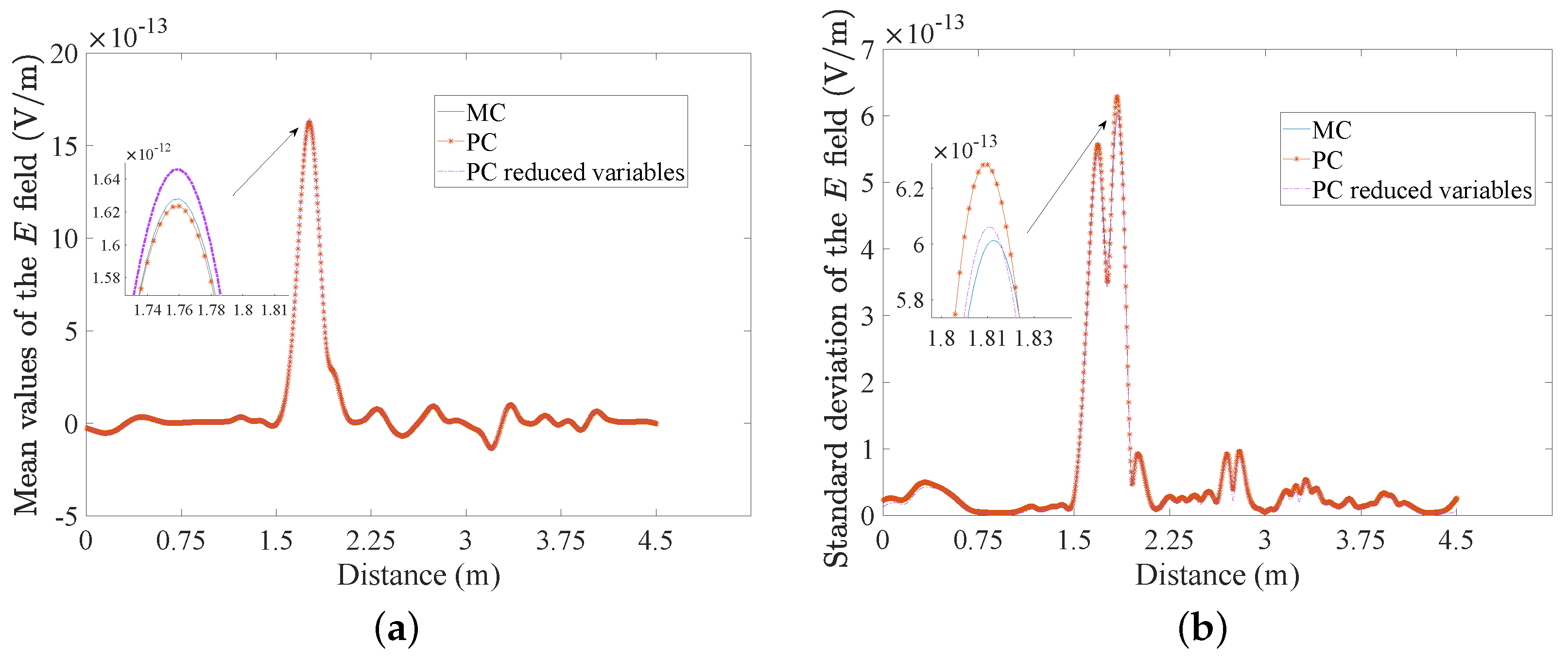
The reduced dimension PC approach was compared with 1000 MC realizations and the original PC method. In this problem, the Morris method required 108 runs for the estimation of the mean elementary effects, which was only a small amount of extra computational burden. The proposed algorithm solved the transmission-line problem using the six most influential variables. The significance of each random input was determined via a threshold, which was equal to $3\times {10}^{-7}$ and was applied in $\mathit{J}$. Therefore, the overall efficiency of the PC algorithm was increased. Figure 2a,b illustrate the mean and the standard deviation of the E field for the first case, respectively. Evidently, the outcomes of the depicted curves were quite satisfactory. In Figure 3, the mean elementary effects are illustrated for each variable of the transmission-line problem for the first case. As already mentioned, the stochastic inputs with high mean elementary effects at a given point in the grid are considered important at that position. In Figure 4a,b, the mean value and the standard deviation of the E field are depicted for the second case. For this scenario, the MC approach required 77 s, while the traditional PC algorithm and the proposed scheme took about 65 s and 38 s, respectively.

The second problem examined the wave propagation within a two-dimensional (2D) space with six concentric dielectric cylinders of infinite length, whose characteristic parameters are shown in

Table 2. Mean dielectric permittivities for the 2D problem.

Dielectric Materials	Mean Dielectric Permittivities
${ϵ}_1$	$8.0{ϵ}_0$
${ϵ}_2$	$2.4{ϵ}_0$
${ϵ}_3$	$5.6{ϵ}_0$
${ϵ}_4$	$4.2{ϵ}_0$
${ϵ}_5$	$6.0{ϵ}_0$
${ϵ}_6$	$7.2{ϵ}_0$

. The computational domain was discretized into $440\times 440$ cells, with a spatial density of 20 cells per wavelength in the vacuum. In this case, a sinusoidal wave was used as a source at 2 GHz, emanating at the center of the domain for 14.142 ns. The dielectric permittivities followed again a uniform distribution, in the range between $\pm 5\%$ of their corresponding mean values. In Figure 5, the geometry of this problem is displayed, where the random materials were positioned apart by $0.075$ m. The first-order Mur’s boundary condition was applied in this case as well. Furthermore, this problem was re-examined, with random inputs ranging between $\pm 10\%$ of their average values. Figure 6a,b depict the mean and the standard deviation of the magnetic field intensity for the “5% percent” case, while Figure 7a,b illustrate the same quantities for the “10% percent” scenario. The results of the proposed method presented a good agreement in this problem as well, as only slight differences were observed, compared to the MC and the standard PC solutions. The simulation time for the MC realizations was approximately 3.28 h (1000 simulations), while the original PC scheme required 1.30 h (389 simulations). However, the proposed PC method needed 44 min (137 runs from the Morris method and 84 runs from the PC scheme with a total of 221 simulations); thus, a speedup of 4.47 compared to the MC method was achieved.

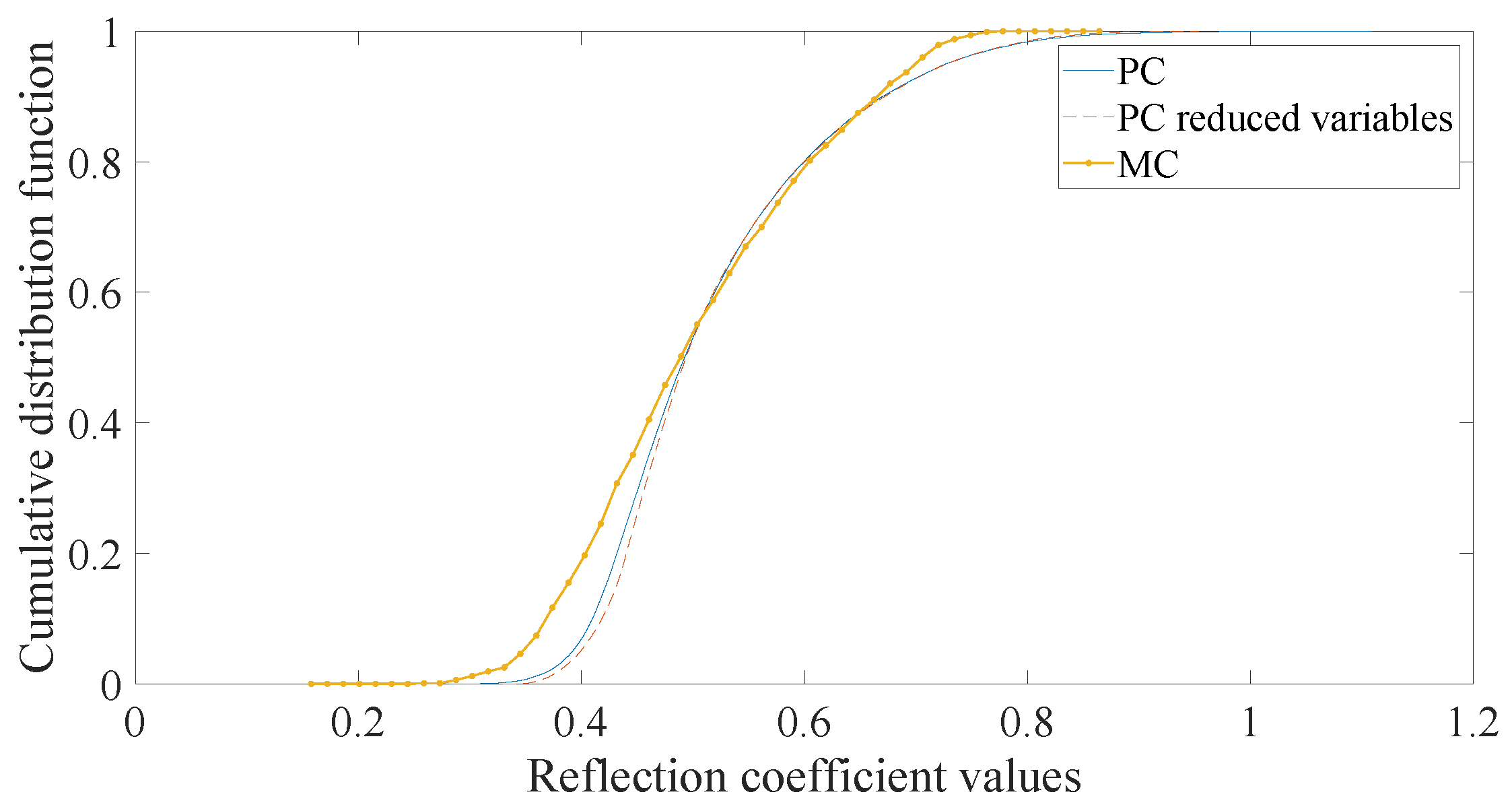
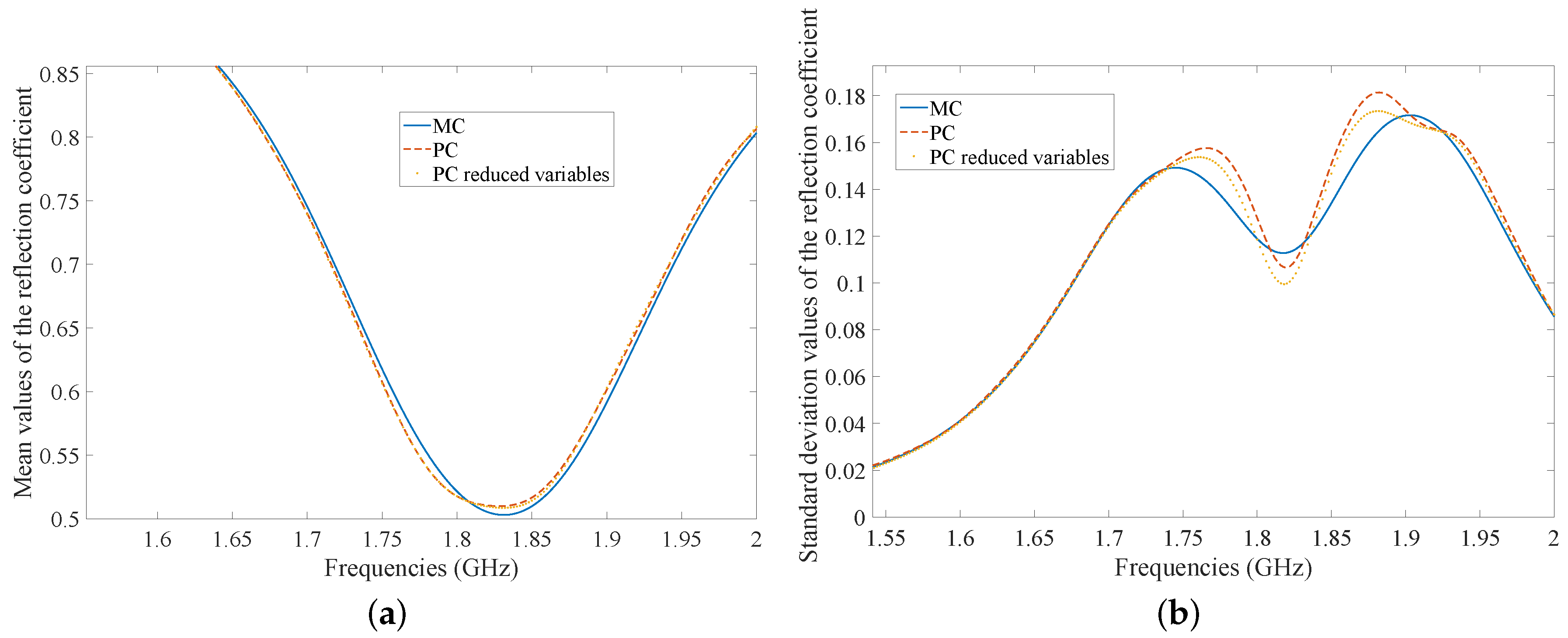
The third problem consists of a patch antenna, the effects of the stochastic inputs on the reflection coefficient (the ratio of the reflected wave to the incident wave at the feeding point of the antenna [23]) of which are examined [24]. In Figure 8, the geometry of the antenna is illustrated, while

Table 3. Mean values and standard deviations for the parameters of the patch-antenna problem.

Parameters	Mean Values	Standard Deviations
$F_i$	$12.5$ mm	$0.360$ mm
$G_{pf}$	$1.0$ mm	$0.028$ mm
$W_f$	$8.5$ mm	$0.245$ mm
W	$51.0$ mm	$1.472$ mm
L	$38.0$ mm	$0.438$ mm
$ϵ$	$4.3{ϵ}_0$	$0.049{ϵ}_0$

depicts the statistical properties of its random quantities. Those quantities followed a uniform distribution. Furthermore, the antenna was excited via a waveguide port, placed at the edge of the microstrip. In this case, the boundaries were terminated via a Perfectly-Matched Layer (PML) [21]. The dimensionality reduction was performed using the three most important variables, which according to the Morris method were the variables W, L, and the permittivity of the dielectric substrate $ϵ$.

In Figure 9, the mean elementary effects of the patch-antenna are displayed, where it is inferred that the aforementioned random variables were the most influential. Furthermore, the mean value, as well as the standard deviation of the reflection coefficient are depicted in Figure 10a,b, respectively. Specifically, it can be concluded that the mean resonance frequency of the patch-antenna was around 1.8 GHz. In Figure 11, the cumulative distribution function (the probability of a stochastic input taking a given value or less [25]) of the reflection coefficient is illustrated around the mean resonance frequency. The presented outcomes displayed a satisfactory agreement; thus, similar results can be extracted with much less computation time. The required simulation time for the traditional PC scheme was around 6 h (389 simulations), and the proposed approach needed 2.33 h (69 simulations from the PC technique and 84 from the Morris method). The MC realizations lasted 15.33 h (1000 simulations). In conclusion, a speedup of 2.57 compared to the standard PC technique has been achieved. The patch-antenna problem was examined again with three additional random inputs: the substrate width $W_{sl}$ (mean value: 102 mm, standard deviation: 8.67 mm), the substrate length $L_{sl}$ (mean value: 76 mm, standard deviation: 4.81 mm), and the substrate height h (mean value: 4.5 mm, standard deviation: 0.01 mm). In this test case, four random variables were considered stochastic, the parameters W, L, $ϵ$, and $L_{sl}$. The remaining ones were treated as deterministic. Figure 12a,b illustrate the mean and the standard deviation for this scenario. In this case, the simulation time of the MC method was about 10 h, while the conventional PC scheme required approximately 18 h. However, the proposed PC approach needed 4 h (137 simulations from the PC technique and 120 realizations from the Morris method); thus, a speedup of 2.5 compared to the MC scheme was achieved.

5. Conclusions

A sensitivity analysis algorithm has been implemented, in order to reduce the computational cost of the PC scheme. The selection of the most important random variables in a given problem can be performed with the proposed heuristic, which is based on the Morris method. The numerical outcomes prove the reliability of the described approach; hence, the efficiency of the PC method can be increased. As future work, a dimensionality reduction of the PC expansion can be performed by combining the Morris method along with anisotropic index sets. Specifically, the indices corresponding to the influential random inputs are more significant than the ones of the trivial stochastic variables. Consequently, the high-order bases, which correspond to the negligible random variables, can be neglected; therefore, the accuracy and the efficiency of the PC method can be further improved.

References

- Tan, T.; Taflove, A.; Backman, V. Single Realization Stochastic FDTD for Weak Scattering Waves in Biological Random Media. IEEE Trans. Antennas Propag. 2013, 61, 818–828. [Google Scholar] [CrossRef] [PubMed]
- Wilke, R.; Slim, J.; Alshrafi, W.; Heberling, D. Polynomial Chaos Expansion as a Tool to Quantify the Performance of the GeReLEO-SMART Satellite Antenna under Uncertainty. In Proceedings of the 2017 International Symposium on Antennas and Propagation (ISAP), Phuket, Thailand, 30 October–2 November 2017; pp. 1–2. [Google Scholar] [CrossRef]
- Hastings, F.D.; Schneider, J.B.; Broschat, S.L. A Monte-Carlo FDTD Technique for Rough Surface Scattering. IEEE Trans. Antennas Propag. 1995, 43, 1183–1191. [Google Scholar] [CrossRef]
- Xiu, D.; Karniadakis, G.E. The Wiener–Askey Polynomial Chaos for Stochastic Differential Equations. SIAM J. Sci. Comput. 2002, 24, 619–644. [Google Scholar] [CrossRef]
- Rong, A.; Cangellaris, A.C. Transient Analysis of Distributed Electromagnetic Systems Exhibiting Stochastic Variability in Material Parameters. In Proceedings of the 2011 XXXth URSI General Assembly and Scientific Symposium, Istanbul, Turkey, 13–20 August 2011; pp. 1–4. [Google Scholar] [CrossRef]
- Austin, A.C.M.; Sarris, C.D. Efficient Analysis of Geometrical Uncertainty in the FDTD Method Using Polynomial Chaos with Application to Microwave Circuits. IEEE Trans. Microw. Theory Tech. 2013, 61, 4293–4301. [Google Scholar] [CrossRef]
- Morris, M.D. Factorial Sampling Plans for Preliminary Computational Experiments. Technometrics 1991, 33, 161–174. [Google Scholar] [CrossRef]
- Salis, C.; Kantartzis, N.; Zygiridis, T. Efficient Stochastic EM Studies via Dimensionality Reduction of Polynomial-Chaos Expansions. In Proceedings of the 2018 7th International Conference on Modern Circuits and Systems Technologies (MOCAST), Thessaloniki, Greece, 7–9 May 2018; pp. 1–4. [Google Scholar] [CrossRef]
- Smolyak, S. Quadrature and Interpolation Formulas for Tensor Products of Certain Classes of Functions. Dokl. Akad. Nauk SSSR 1963, 148, 1042–1045. [Google Scholar]
- Beddek, K.; Clenet, S.; Moreau, O.; Costan, V.; Menach, Y.L.; Benabou, A. Adaptive Method for Non-Intrusive Spectral Projection—Application on a Stochastic Eddy Current NDT Problem. IEEE Trans. Magn. 2012, 48, 759–762. [Google Scholar] [CrossRef]
- Ma, X.; Zabaras, N. An Adaptive Hierarchical Sparse Grid Collocation Algorithm for the Solution of Stochastic Differential Equations. J. Comput. Phys. 2009, 228, 3084–3113. [Google Scholar] [CrossRef]
- Blatman, G.; Sudret, B. Adaptive Sparse Polynomial Chaos Expansion Based on Least Angle Regression. J. Comput. Phys. 2011, 230, 2345–2367. [Google Scholar] [CrossRef]
- Peng, J.; Hampton, J.; Doostan, A. A Weighted L1-Minimization Approach for Sparse Polynomial Chaos Expansions. J. Comput. Phys. 2014, 267, 92–111. [Google Scholar] [CrossRef]
- Diaz, P.; Doostan, A.; Hampton, J. Sparse Polynomial Chaos Expansions via Compressed Sensing and D-Optimal Design. Comput. Methods Appl. Mech. Eng. 2018, 336, 640–666. [Google Scholar] [CrossRef]
- Zhang, Z.; Weng, T.W.; Daniel, L. Big-Data Tensor Recovery for High-Dimensional Uncertainty Quantification of Process Variations. IEEE Trans. Compon. Packag. Manuf. Technol. 2017, 7, 687–697. [Google Scholar] [CrossRef]
- Zhang, Z.; Yang, X.; Oseledets, I.V.; Karniadakis, G.E.; Daniel, L. Enabling High-Dimensional Hierarchical Uncertainty Quantification by ANOVA and Tensor-Train Decomposition. IEEE Trans. Comput.-Aided Des. Integr. Circuits Syst. 2015, 34, 63–76. [Google Scholar] [CrossRef]
- Xiu, D. Numerical Methods for Stochastic Computations: A Spectral Method Approach; Princeton University Press: Princeton, NJ, USA, 2010. [Google Scholar]
- Aiouaz, O.; Lautru, D.; Wong, M.F.; Conil, E.; Gati, A.; Wiart, J.; Hanna, V.F. Uncertainty Analysis of the Specific Absorption Rate Induced in a Phantom Using a Stochastic Spectral Collocation Method. Ann. Telecommun. Ann. Des Télécommun. 2011, 66, 409–418. [Google Scholar] [CrossRef]
- Clenshaw, C.W.; Curtis, A.R. A Method for Numerical Integration on an Automatic Computer. Numer. Math. 1960, 2, 197–205. [Google Scholar] [CrossRef]
- Campolongo, F.; Cariboni, J.; Saltelli, A. An Effective Screening Design for Sensitivity Analysis of Large Models. Environ. Model. Softw. 2007, 22, 1509–1518. [Google Scholar] [CrossRef]
- Taflove, A.; Hagness, S.C. Computational Electrodynamics: The Finite-Difference Time-Domain Method; Artech House: Norwood, MA, USA, 2005. [Google Scholar]
- Mur, G. Absorbing Boundary Conditions for the Finite-Difference Approximation of the Time-Domain Electromagnetic-Field Equations. IEEE Trans. Electromagn. Compat. 1981, EMC-23, 377–382. [Google Scholar] [CrossRef]
- Bowick, C. RF Circuit Design Approach; Newness: Oxford, UK, 1997. [Google Scholar]
- Salis, C.; Zygiridis, T. Dimensionality Reduction of the Polynomial Chaos Technique Based on the Method of Moments. IEEE Antennas Wirel. Propag. Lett. 2018, 17, 2349–2353. [Google Scholar] [CrossRef]
- Park, K., II. Fundamentals of Probability and Stochastic Processes with Applications to Communications; Springer: Holmdel, NJ, USA, 2018. [Google Scholar]
Figure 1.
Geometric features of the 1D transmission-line problem.
Figure 2.
(a) Mean value and (b) standard deviation of the electric field for the first case of the 1D transmission-line problem. PC, Polynomial Chaos.
Figure 3.
Mean elementary effects for each random variable in the first case of the 1D transmission-line problem.
Figure 4.
(a) Mean value and (b) standard deviation of the electric field for the second case of the 1D transmission-line problem.
Figure 5.
Geometric features of the 2D problem.
Figure 6.
(a) Mean value and (b) standard deviation of the magnetic field for the first case of the second problem.
Figure 7.
(a) Mean value and (b) standard deviation of the magnetic field for the second case of the second problem.
Figure 8.
Schematic of the patch-antenna problem.
Figure 9.
Mean elementary effects of the path-antenna problem for the first case.
Figure 10.
(a) Mean value and (b) standard deviation of the reflection coefficient for the first case of the path-antenna problem.
Figure 11.
Cumulative distribution function for the first case of the patch-antenna problem.
Figure 12.
(a) Mean value and (b) standard deviation of the reflection coefficient for the second case of the path-antenna problem.