China’s Bank Balance Sheet and Financing of Heterogeneous Enterprises

Abstract

Given the background of financial disintermediation and interest rate marketization, the assets of China’s commercial banks can be divided into traditional credit assets, whose rates of return are controlled by the supervision department, and financial assets, whose rates of return fluctuate according to market conditions. Direct financing enterprises are mainly state-owned enterprises with a good reputation, endorsed by the government, and they finance using the financial assets of commercial banks. Indirect financing enterprises are mainly private enterprises, which finance using credit assets. By introducing a financial intermediary sector with a balance sheet into dynamic stochastic general equilibrium (DSGE) model, our model endogenously determines the leverage ratio and the ratio of the two assets of the bank. Model results show that the impact from the volatility of financial markets and other exogenous shocks can affect the banks’ asset proportions of the two asset types, asymmetrically affecting the production scale of enterprises with two types of financing. Further, the bank’s leverage ratio changes will have a magnifying effect on economic fluctuations.

1. Introduction

1.1. Increasing Attention to Financial Institutions’ Balance Sheets

In the international market, the global financial crisis of 2008 has once again focused increasing attention on financial institutions’ balance sheets. Many scholars have studied the amplification effect of the financial sector’s balance sheet deterioration in the process of fermentation and spread of the financial crisis. As proposed by the International Monetary Fund (IMF 2008), the subprime mortgage crisis in the United States reflects the weakness in the balance sheet. Yan (2008) stated that the root cause of this crisis was the decline in the balance sheet of individuals and the banking sector. The subprime crisis was not a crisis of overcapacity, but essentially a financial institution’s balance sheet crisis, as pointed out by Li and Song (2009).

In China’s financial market, due to the impact of decreasing macroeconomic growth, financial disintermediation, and interest rate liberalization in recent years, the traditional credit business of commercial banks is facing greater challenges, and the previous high profit level of the banking industry has gradually fallen, driving the domestic banking industry into the stage of “differentiated” competition. Bank assets continue to tilt toward investment in securities such as stocks and bonds. The diversification of bank assets poses new challenges for commercial bank risk management and provides a new channel for the financing of the real economy.

Therefore, studying new changes in bank balance sheets will help understand the impact of financial system stability on real economy financing. It has positive significance for defusing financial risks and achieving the goal of finance that serves the real economy.

1.2. New Changes in Bank’s Balance Sheets

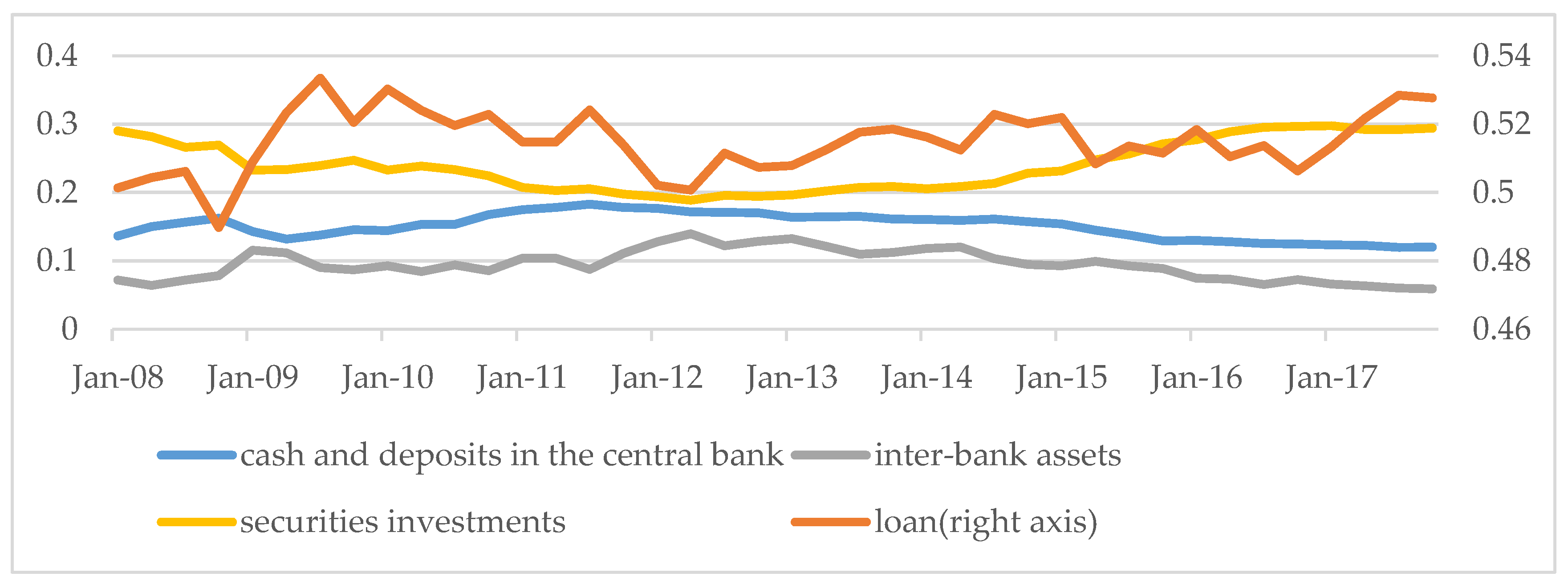
According to the characteristics of a bank’s assets, the assets can be divided into four categories: cash and deposits in the central bank, inter-bank assets, loans, and securities investments. In addition, a bank’s asset-side subjects include precious metals, derivative financial assets, long-term equity investments, etc. Because the proportion of these assets does not exceed 5% of the total assets, and has no significant impact on the daily operations of the bank, these were not considered here. Inter-bank assets include due from other banks, lending funds, and redemptory monetary capital for sale. Securities investments include trading financial assets, available-for-sale financial assets, held-to-maturity investments, and receivables. Receivables are mainly interbank deposit receipts, wealth management products, and trusts. The asset proportion of different commercial banks are slightly different.

Figure 1 shows the trend in the proportion of bank assets. The loan is still the largest proportion of assets held by commercial banks. Since 2010, the central bank has raised the deposit reserve ratio of commercial banks in order to alleviate inflationary pressures. Tight monetary policy has gradually reduced the proportion of loans. In 2015, the regulatory authorities continuously issued documents to regulate the development of inter-bank business. Inter-bank assets have been shrinking since then, and the scale of securities assets, which can be seen as a substitute for interbank assets, continues to rise simultaneously. Overall, the proportion of loans fluctuated around 49%, and the proportions of securities assets and inter-bank assets were around 25% and 10%, respectively. With the continuous advancement in financial disintermediation and interest rate liberalization, financial assets such as securities have become the most important asset for commercial banks besides loans.

According to Wind database, by the end of March 2018, the total size of China’s bond market was 76 trillion CNY. The interest rate debt was about 41 trillion, the credit bond was 25.6 trillion, and the interbank deposit was 8.6 trillion. The size of the bonds held by commercial banks, the most important player in the bond market, was about 36.8 trillion, accounting for 48.4% of the total bond market.

In summary, the change in the bank’s assets is that the proportion of traditional credit is gradually decreasing, while the proportion of financial assets—such as bonds—is gradually increasing. Therefore, this paper divides bank assets into credit assets and financial assets. Credit assets refer to the traditional loans of banks, which are characterized by the loan interest rate being subject to supervision and cannot float freely. The total amount of credit assets is b_t and the loan interest rate is $R_t^b$. Financial assets refer to assets held by banks that can be publicly traded in financial markets, such as bonds, stocks, and interbank deposit certificates. The characteristic of financial assets is that asset prices Q_t (and corresponding financial asset yields $R_t^k$) are not controlled by regulatory authorities, but rather, are affected by the macroeconomic environment and can fluctuate with market conditions. The amount of financial assets held by banks is s_t. It is thought that this setting can, to some extent, capture the unique dual interest rate system in China’s financial system.

1.3. Reasons for Changes in Balance Sheets

The reasons for these new changes in terms of the bank’s assets are both from the bank—the supply side of the funds, and from the enterprise—the demand side of the funds. The following is an overview of these reasons from both the bank and the enterprise.

1.3.1. Banks—The Supply Side of the Funds

From the experience of international banking development, financial mixed operation has become an important means to improve the competitiveness of the banking industry and achieve economies of scope. In 2006, China’s “Eleventh Five-Year Plan” proposed to promote the integration of the financial industry. Commercial banks, through acquisitions and setting new subsidiaries, have gradually held licenses for public funds, financial leasing, insurance, securities, and trusts (Zheng 2016). Mixed operation has broken the original pattern of “Bank, Securities, Insurance” which means divided operation, leading to business interpenetration between banks and non-bank financial institutions, and changing the characteristics of capital flow and the structure of assets and liabilities. The proportion of investment, equity, and intermediate business on the balance sheet will gradually increase. In this context, besides the traditional deposit and loan business, the business of investment and loan linkage, asset management, and credit asset transfer become important measures for commercial banks, to expand their business operations, innovate investment channels, and increase profits.

The unique dual track interest rate system of China’s financial system still exists. Before 2015, the deposit and loan interest rates of commercial banks were both regulated. After 2015, with the advancement of interest rate marketization, although the government has already assigned pricing power of deposit and loan interest rates to commercial banks, deposit and loan interest rates are still governed by the supervision department’s window guidance. Similarly, the market interest rate is dominated by the self-disciplined market interest rate pricing mechanism. The loan interest rate can only be adjusted within a certain range. This results in the bank’s earnings from loans cannot match the risk the bank undertakes, and the development of traditional credit business is greatly limited. In contrast, when banks allocate funds to financial markets, as a financial intermediary, the bank’s information superiority, professional, and technological advantages, makes it think that operating financial assets can obtain higher returns than traditional credit, although they have to bear the risks of financial markets.

The bank enriches the asset side in order to meet the capital adequacy requirements. The capital adequacy ratio is an important indicator that commercial banks need to address in asset management, and is an important constraint for supervisory authorities to control bank management risks. In order to meet the capital adequacy ratio requirements, commercial banks either increase bank capital or reduce the proportion of high-risk assets, and allocate more assets to low-risk assets (Ming et al. 2017). This means that issuing preferential stocks and subordinated debts to increase bank capital is difficult in the short term. Therefore, in order to meet regulatory requirements in a short period, banks can only adjust the current asset structure and reduce the proportion of high-risk assets. According to the Measures for Capital Management of Commercial Banks, the risk weight of national debt and policy financial bonds is 0, the risk weight of local government bonds is 20%, the risk weight of interbank deposit certificates is 25%, and the risk weight of general enterprises is 100%. In order to meet regulatory requirements, banks allocate assets in bonds, which can reduce the capital occupation of banks and better meet the capital adequacy ratio requirements.

In addition, compared with loans, interest bonds such as government bonds have a tax advantage. The issuance of interest-rate bonds, such as treasury bonds and local government bonds, are not subject to value-added tax and income tax, while the issuance of loans are subject to value-added tax at a rate of 6%, and income tax is 25%.

1.3.2. Enterprises: The Demand Side of Funds

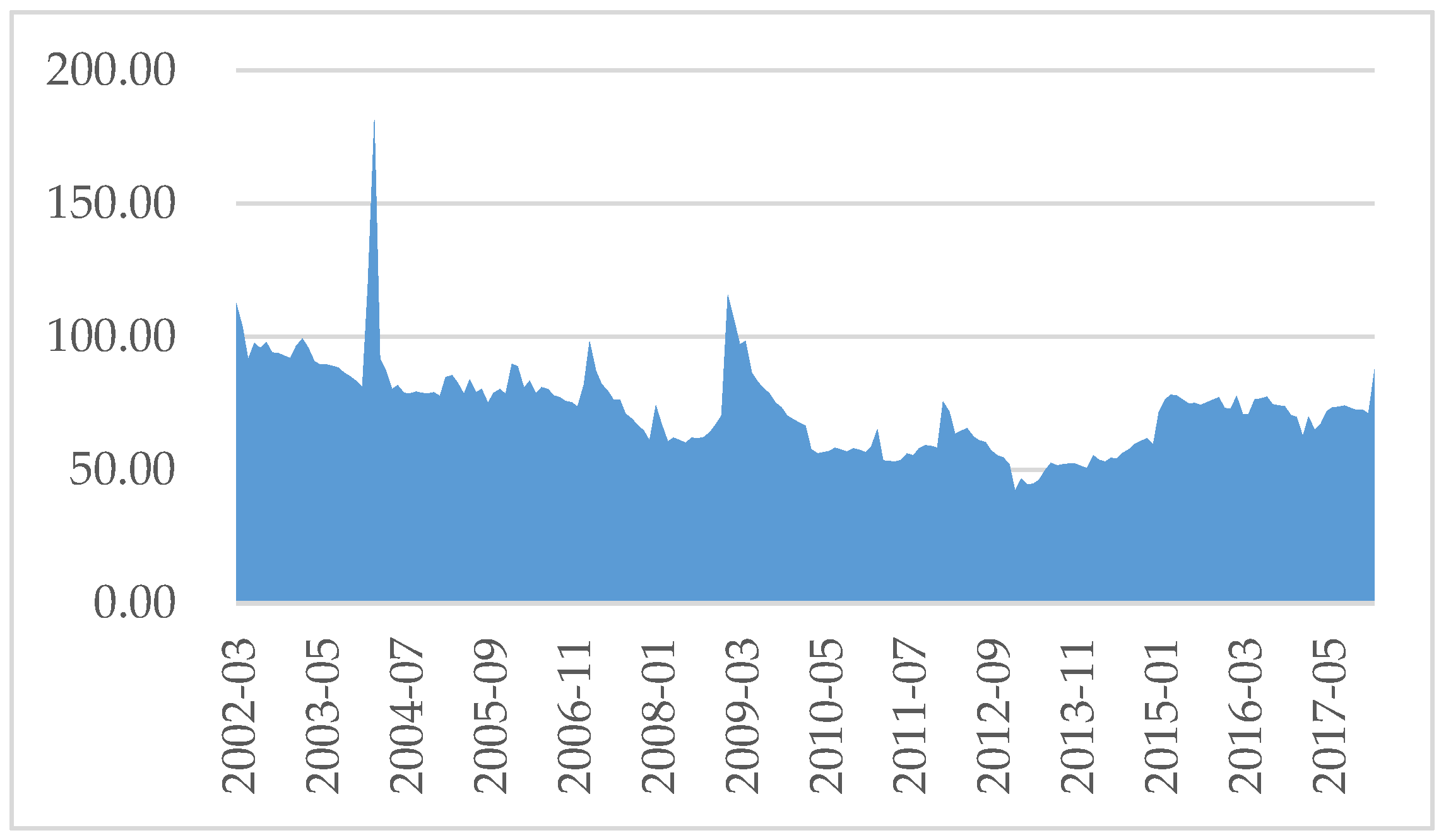
The local government financing model has changed. As shown in Figure 2, the proportion of traditional credit in social aggregate financing has declined. The main reason for this is that the local government changed their financing channel. Yi (2017) proposed that the original financing channel is that banks provide credit for enterprises with government background. However, after the introduction of the new Budget Law and State Council’s Opinions on Strengthening Local Government Debt Management, the local government financing model has changed significantly. Bank loans are gradually replaced by government bonds. The pattern where banks participate in local infrastructure construction by loans to business will be hard to sustain. Thus, commercial banks must transition from being financing-oriented businesses to investment-oriented or intermediary-oriented businesses.

The national industrial structure has been transformed and upgraded into a pattern of light assets. At present, China’s economic and industrial structure has undergone a significant change. The added value of the tertiary industry accounts for almost half of the gross domestic product (GDP). Heavy industries with high energy consumption, heavy assets, and low efficiency are gradually being substituted by clean, light assets and intelligence (Yi 2017). Specifically, the market space of the light asset industry, such as the Internet, medicine, cultural education, media, and entertainment, is becoming increasingly extensive. The heavy asset industries, such as steel, coal, and cement, are under tremendous pressure to de-capacity and simplify assets. In the process of light asset transformation, it is difficult for enterprises to connect business, such as research and development (R&D) investment, integrating operational resources, and mergers and acquisitions, with traditional bank loan business. This scenario has placed urgent requirements for the bank to establish a comprehensive financial service framework for stocks, bonds, and loans.

Based on the above, studying the changes in bank balance sheets in recent years will help analyze the stability of China’s financial system and financial fluctuations. Therefore, this paper intends to include the commercial bank’s balance sheet as representative of the financial sector in the mainstream macroeconomic model (DSGE) to examine its impact on China’s macro finance.

1.4. Contribution of This Paper

Different from previous research on macro finance, this paper mainly introduces improvements in the following three aspects. Firstly, in view of the above characteristics of financial markets, such as the dual-track interest rate system specific to China, this paper, for the first time, includes the characteristics of bank assets into the DSGE model to analyze the impact of external factors, such as financial market impact and technological impact, on China’s macro economy. Specifically, bank assets are divided into financial assets and credit assets. The price of financial assets is directly affected by the fluctuations in the financial market, so the rate of return can be flexible. The rate of return on credit assets, namely the interest rate on loans, is controlled by regulators and cannot float freely. Secondly, according to the unique enterprise nature in China, this paper applies the demand side of credit assets, namely indirect financing enterprises, to large state-owned enterprises. The demand side of financial assets—direct financing enterprises—corresponds to private small to medium size enterprises (SMEs). The main reason for the differences in financing channels between state-owned enterprises and private enterprises is that the yield characteristics of credit assets and financial assets are different. Unlike state-owned enterprises, private SMEs have no government guarantee and are highly risky. However, regulated lending rates cannot be adjusted to match the risks of private enterprise. Therefore, enterprises with different ownership attributes choose different financing methods. This paper clearly describes this macroeconomic feature of China. Thirdly, according to the DSGE model that reflects the characteristics of China’s financial market constructed in this paper, the results of this paper enrich the balance sheet channels in the existing monetary policy transmission mechanism. Empirical results, such as impulse response function, show that transmission channels are similar to the traditional financial amplifier mechanism. Specifically, by introducing the financial intermediary sector with a balance sheet into the DSGE model, the model can endogenously determine a bank’s leverage ratio and the holding ratio of the bank’s two types of assets. The shock from the financial market will affect the proportion of financial assets and credit assets held by the bank, and then asymmetrically impact the production scale of the two types of financing enterprises. Through the changes in the bank’s leverage ratio, the macroeconomic fluctuations are amplified.

2. Literature Review

In early macro-financial literature, modeling ideas mainly concentrated on the credit demand side, whereas the banking sector and its behavior as credit providers were rarely characterized. Before the subprime mortgage crisis, the DSGE model, based on the financial accelerator and collateral constraint mechanism, did not explicitly include a banking sector. For example, Iacoviello (2005) introduced the mortgage constraint mechanism into the DSGE model as the manifestation of financial friction. Then, he assumed the real estate price as an important asset price affecting the real economy and analyzed the transmission channel of monetary policy. After the crisis, DSGE modeling on bank capital mechanisms continued to develop.

Goodfriend and McCallum (2007) introduced a perfectly competitive banking sector into the DSGE based on the BGG model. The article introduced the banking sector to describe the differences and interactions between different types of interest rates. In this article, the asset side of the bank’s balance sheet is the loan and the base currency, and the liability side is the deposit. In the model of Meh and Moran (2010), the existence of bank capital can alleviate the agency problem between banks and depositors, which affects the accumulation of loanable funds (deposits), which in turn affects the expansion and contraction of the economy. In the model of Gertler and Karadi (2011), there is a moral hazard problem between banks and depositors, so that an incentive compatibility constraint was introduced. This constraint makes the banking sector’s leverage endogenous and links bank capital to external financing premiums. In the model’s balance sheet, the asset side is the financial assets held by the bank, and the liability side is the deposits and bank capital. Dib (2009) examined the role of financial friction in the interbank market. The banking sector in the article included two heterogeneous sub-sectors. Loans consisted of borrowings and bank capital in the interbank market. Banks have monopoly power so that they can specify deposit and loan interest rates. Bank capital was introduced in order to meet capital requirements as a collateral for the interbank market. The interbank market model (Gertler and Kiyotaki 2010) focused on the impact of changes in the value of capital held by banks on the interbank market lending and bank balance sheets. In this model, the decline in the value of capital reduces the value of assets held by banks, which also reduces their borrowing capacity. The reduction in borrowing capacity further reduces the demand for corporate assets, thereby further reducing the value of corporate capital. In the bank balance sheet established by Gertler and Kiyotaki (2010), the debt side has newly added interbank market loans. Gertler et al. (2012) added bank equity financing to the liability side of the bank’s balance sheet, which in turn made the bank’s risk exposure endogenous.

In domestic research, Kang and Gong (2014) introduced the bank’s balance sheet into the DSGE model in an open economy, and divided the enterprise into heterogeneous export and non-export enterprises. They studied how the international economic crisis affects a country’s exports, which in turn caused a loss of bank assets in China. Liu and Yao (2016) introduced exogenous factors, such as asset price shocks, into the DSGE model within the financial sector to explore the impact of these exogenous shocks on monetary policy goals. Wang and Tian (2016) established a heterogeneous banking sector in which the defaulted probability of interbank market was endogenous, and then discussed the impact of capital regulation on systemic financial risks.

Overall, the existing literature mainly focused on bank capital in the balance sheet. However, these studies simply regarded a bank’s asset side as one single asset, such as loans. There are a handful of articles involving financial assets, and even fewer articles have included credit assets and financial assets simultaneously. The theoretical model of this paper is mainly based on Gertler and Karadi (2011) and Iacoviello (2005). The model in this paper is solved using the value maximization problem following the method introduced by Gertler and Karadi (2011). We also introduce the mortgage constraint mechanism, which is similar to Iacoviello (2005). However, this model is different from both previous studies. Iacoviello (2005) focused on the impact of the real estate market and mortgage constraint mechanisms on the economy, and did not explicitly introduce the financial sector in the model. Gertler and Karadi (2011) did not distinguish heterogeneous production enterprises or bank assets; this paper describes both in detail and analyzes the impact on the macro economy.

Generally, traditional credit assets are strictly regulated and the price of credit assets is, to some extent, rigid. In contrast, the categories of financial assets held by banks are constantly enriched and the size of financial assets are expanding. The price of financial assets freely vary with market conditions. Therefore, this paper focuses on the latest changes in the balance sheet of China’s commercial banks, enriches the asset-side setting, and incorporates credit assets and financial assets into the balance sheet simultaneously to examine the impact of exogenous shocks on the economy.

3. Theoretical Model

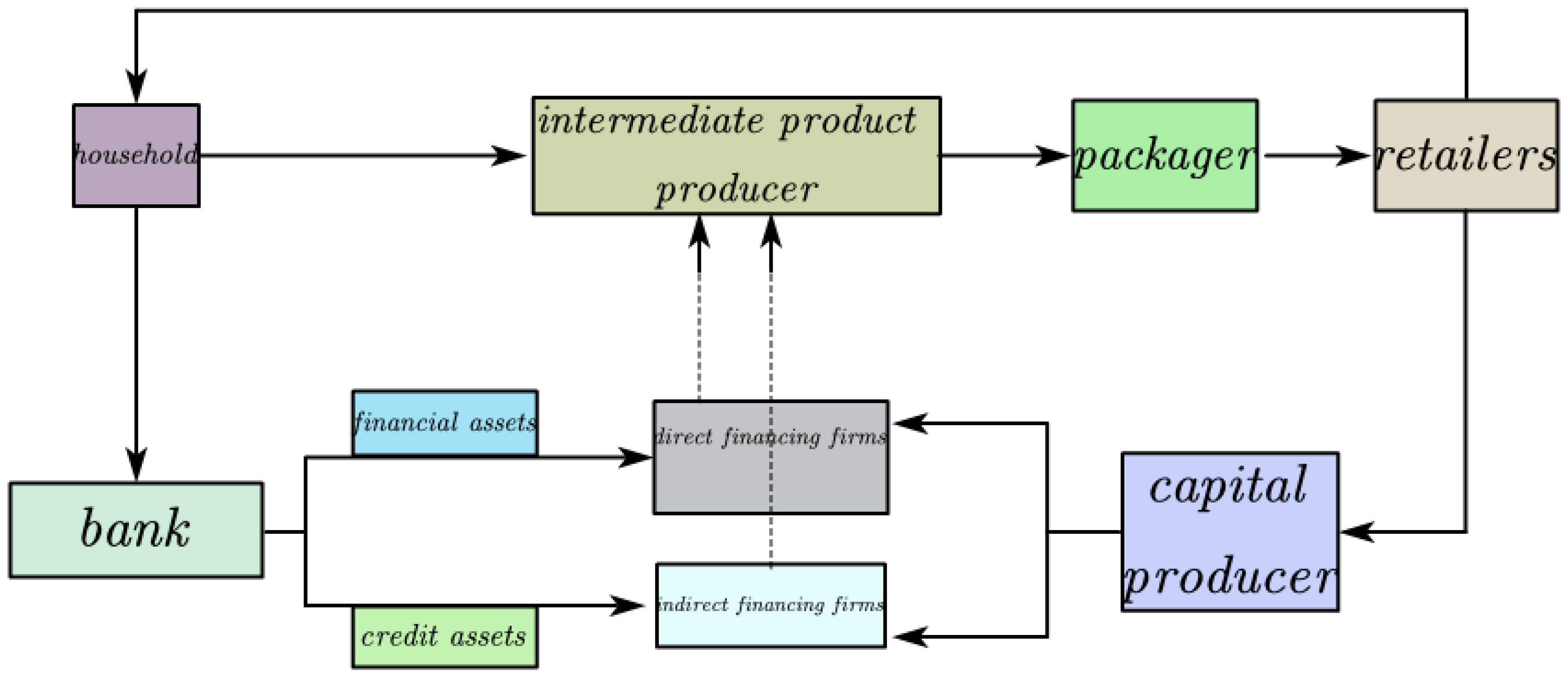
This paper constructs a new Keynesianism- dynamic stochastic general equilibrium (NK-DSGE) model, which is shown in Figure 3. The household provides labor to intermediate producers and provides savings to the banking sector. Banks then allocate deposits to two types of intermediate producers: direct financing enterprises and indirect financing enterprises. Indirect financing enterprises are mainly state-owned. Loan is the financing method for such enterprises. Direct financing enterprises are mainly small- and medium-sized private enterprises, which are high risk and cannot obtain financing support from the traditional bank loan channel. They can only issue bonds in the financial market for financing. The products of intermediate enterprises are sold to the packager. The packager packages the goods and sells them to the retailer. The purpose of introducing retailers is to introduce price stickiness. The retailer sells the final product to the household for consumption and to the capital producers for investment. The following sections describe the detailed settings of the model.

3.1. Household

Suppose there is a continuum of homogeneous households, each of which consumes, saves, and provides labor. Each household consists of two types of members: workers and bankers. Workers provide labor and earn wages for the family; bankers manage financial intermediaries (banks), so the family is the owner of the bank and the profits earned are returned to the family. Within a representative household, the proportion of bankers is f and the proportion of workers is 1 − f.

In particular, bankers face a survival probability σ in each period. At the end of each period, the bank has the probability σ of entering the next phase. σ is independent of historical distribution. Whether the banker can enter the next period has nothing to do with how many years they have survived in the economy. Through this assumption, the average survival time of bankers is 1/(1 − σ). The reason why the banker’s limited-term survival hypothesis was introduced is to prevent bankers from accumulating sufficient profits so that they can fund all investment from their own capital.

In each period, there are (1 − σ)f bankers who exit from financial intermediation activities and become workers. In order to maintain the ratio of bankers and workers, we assumed that a similar number of workers become bankers in each period, and the family provides the start-up funds needed for new bankers to carry out financial intermediation activities. We introduce this when introducing financial intermediaries. The optimization issue for representative families is as follows:

$$\begin{array}{l}Max{E}_t{\displaystyle \sum _{i=0}^{\infty }\left[\ln \left(C_{t+i}-h{C}_{t+i-1}\right)-\frac{\chi }{1+\phi }{L}_{t+i}^{1+\phi }\right]}\\ s.t.P_t{C}_t=W_t{L}_t+{\Pi }_t^H+T_t+R_t{D}_{t-1}-D_t\end{array}$$

(1)

where, in the objective function, $C_t$ represents the consumption of the family, $L_t$ represents the labor supply of the family, $\beta$ is the intertemporal discount factor of the family, $h$ is the parameter that controls the inertia of consumption, $\phi$ is the reciprocal of the Frisch labor supply elasticity, and $\chi$ indicates the weight of the utility of labor. In the budget constraint equation of representative households, $P_t$ is the price level, $W_t$ is the nominal wage, ${\Pi }_t^H$ is the profit that the family obtains from the ownership of financial intermediaries and non-financial enterprises, $T_t$ is lump sum taxes, $D_t$ is the total amount of deposits at the beginning of the period, and $R_t$ is the nominal total rate of return of the deposit $D_{t-1}$ from the beginning of the period $t-1$ to the beginning of the period $t$. Therefore, $R_t{D}_{t-1}$ is the total income of the household in the current period. ${\Pi }_t={P_t/P}_{t-1}$ indicates the rate of inflation. We can obtain the first-order condition of the family optimization issue:

$$\begin{array}{l}{P}_t{\lambda }_t^h=\left[{(C_t-h{C}_{t-1})}^{-1}-\beta h{E}_t{(C_{t-1}-h{C}_t)}^{-1}\right]\\ {\lambda }_t^h{W}_t=\chi L_t^{\phi }\\ E_t\left({\Lambda }_{t,t+1}{R}_{t+1}\right)=1,{\Lambda }_{t,t+1}=\frac{{\lambda }_{t+1}^h}{{\lambda }_t^h}\beta \end{array}$$

(2)

3.2. Bank

3.2.1. Bank Balance Sheet

In the financial market, commercial banks play the role of an intermediate between the supply and demand of funds. Banks can obtain funds from two sources: their own retained earnings and household deposits. Both are the two types of funds that comprise the liability side of the bank’s balance sheet. Banks can invest in two ways: a credit asset and a financial asset. At the beginning of the period t, the bank issues credit $b_t$ for one period to the enterprise, and gains the nominal total rate of return $R_{bt+1}$ when the loan expires at the end of period t. The number of bonds issued by the bank is affected by the value of the mortgageable assets of the enterprise. Similarly, the amount of financial assets issued by the bank is $S_t$ and the price is $Q_t$. Unlike credit assets, the yield of financial assets $R_{kt+1}$ is flexible, depending on the performance of the financial market. In short, a bank’s balance sheet can be seen as the following equation:

$$Q_t{s}_t+b_t=n_t+d_t$$

(3)

3.2.2. Evolution of the Bank’s Net Worth $n_t$

The change in a bank’s equity capital $n_t$ depends on the difference between the asset’s return and the cost of deposit:

$$n_t=R_{kt}{Q}_{t-1}{s}_{t-1}+R_{bt}{b}_{t-1}-R_t{d}_{t-1}$$

(4)

We substituted the balance sheet equation into the above formula, eliminated $d_t$, and obtained the equation as follows:

$$\begin{array}{l}{n}_t=R_{kt}{Q}_{t-1}{s}_{t-1}+R_{bt}{b}_{t-q}-R_t\left(Q_{t-1}{s}_{t-1}+b_{t-1}-n_{t-1}\right)\\ =\left(R_{kt}-R_t\right)Q_{t-1}{s}_{t-1}+\left(R_{bt}-R_t\right)b_{t-1}+R_t{n}_{t-1}\end{array}$$

(5)

Assume that the ratio of credit assets to financial assets is $x_t$, i.e., substituting $x_t$ into the above formula, eliminating $b_t$, and obtaining the evolution of $n_t$ produces:

$$\begin{array}{l}{n}_t=\left(R_{kt}-R_t\right)Q_{t-1}{s}_{t-1}+\left(R_{bt}-R_t\right)x_{t-1}{Q}_{t-1}{s}_{t-1}+R_t{n}_{t-1}\\ =\left[\left(R_{kt}-R_t\right)+\left(R_{bt}-R_t\right)x_{t-1}\right]Q_{t-1}{s}_{t-1}+R_t{n}_{t-1}\end{array}$$

(6)

3.2.3. Moral Hazard Problem

Given the banker’s financial constraints, they are motivated to keep all profits until they exit. When they exit, they will spend all their accumulated funds. Therefore, the banker’s goal is to maximize the expected discounted value of their future final dividend:

$$V_t=E_t\left({\displaystyle \sum _{i=0}^{\infty }\left(1-\sigma \right){\sigma }^{i-1}{\Lambda }_{t,t+i}{n}_{t+i}}\right)$$

(7)

because the rates of return $R_{bt}$ and $R_{kt}$ are higher than the interest rate paid to depositors $R_t$. Bankers have the incentive to indefinitely absorb deposits from households and expand their assets. In order to limit the ability of bankers to unrestrictedly expand their assets, we introduced a moral hazard problem: when a banker receives funds, they can divert a certain proportion of this fund for private use. When households are aware of this situation, they will not deposit money into the intermediary without restriction. The cost of the banker diverting the deposit for other purposes, is that the depositor can force the bank to go bankrupt and liquidate, thereby obtaining the net value of the remaining portion $\left(1-\theta \right)$ of the bank.

If the household is willing to deposit money into an intermediary, the net value of the bank must be greater than the value it would have obtained by diverting the deposit for private use. The incentive compatibility constraint is the following:

$$V_t\ge \theta \left(x_t\right)\left(Q_t{s}_t+b_t\right)$$

(8)

Notably, we assumed that the proportion of funds $\theta$ that bankers can divert is a function of $x_t$, $\theta \left(x_t\right)=\theta \left(\eta x_t+\kappa \right)$. The yield on credit assets is relatively fixed. It is easier for households to monitor the payment and default of credit. However, there is a large degree of uncertainty in the return of financial assets. Bankers can more easily divert financial assets in the financial market for private purposes, while attributing the loss of financial assets to financial market risks. Therefore, the larger the $x_t$, the higher the credit assets proportion, and the lower the proportion of funds $\theta$ that bankers can divert, i.e., $\eta <0$. Substituting the expression of $x_t$ into $\theta \left(x_t\right)$, the constraint is:

$$V_t\ge \theta \left(\eta x_t+\kappa \right)\left(1+x_t\right)Q_t{s}_t$$

(9)

3.2.4. Bank Optimization

Bank optimization can be expressed as follows:

$$s.t.\hspace{1em}\hspace{1em}\begin{array}{l}{V}_t\left(s_t,x_t,n_t\right)=E_t{\Lambda }_{t,t+1}\left\{\left(1-\sigma \right)n_{t+1}+\sigma \underset{s_{t+1}{x}_{t+1}}{\max }\left[V_{t+1}\left(s_{t+1},x_{t+1},n_{t+1}\right)\right]\right\}\\ n_t=\left[\left(R_{kt}-R_t\right)+\left(R_{bt}-R_t\right)x_{t-1}\right]Q_{t-1}{s}_{t-1}+R_t{n}_{t-1}\\ V_t\ge \theta \left(\eta x_t+\kappa \right)\left(1+x_t\right)Q_t{s}_t\end{array}$$

(10)

The first order conditions can be obtained as follows (due to space limitation, the solution process is not detailed here; contact the author if necessary):

$$\begin{array}{l}{\mu }_{st}=E_t\left[{\Lambda }_{t,t+1}{\Omega }_{t+1}\left(R_{kt+1}-R_{t+1}\right)\right]\\ {\mu }_{bt}=E_t\left[{\Lambda }_{t,t+1}{\Omega }_{t+1}\left(R_{bt+1}-R_{t+1}\right)\right]\\ {\upsilon }_t=E_t\left[{\Lambda }_{t,t+1}{\Omega }_{t+1}{R}_{t+1}\right]\end{array}$$

(11)

$$\begin{array}{l}{\Omega }_{t+1}=\left(1-\sigma \right)+\sigma \left(\left({\mu }_{st+1}+x_{t+1}{\mu }_{bt+1}\right){\psi }_{t+1}+{\upsilon }_{t+1}\right)\\ {\psi }_t=\frac{Q_t{s}_t}{n_t}=\frac{{\upsilon }_t}{\theta \left(1+x_t\right)\left(\eta x_t+\kappa \right)-\left({\mu }_{st}+x_t{\mu }_{bt}\right)}\end{array}$$

(12)

$$\frac{1}{2}{x}_t+\frac{{\mu }_{st}}{{\mu }_{bt}}=\frac{\eta +\kappa }{4\eta }+\frac{\kappa -\left(\eta +\kappa \right)/4\eta }{2\eta x_t+\eta +\kappa }$$

(13)

where ${\psi }_t=\frac{Q_t{s}_t}{n_t}$ is the ratio of financing assets to the capital of financial intermediate.

3.2.5. Motion Equation of the Total Value of the Bank $N_t$

In the period t, the total value of the bank ($N_t$) is equal to the sum of the net value of the bank that survives from the last period and the new bank that enters in the current period.

$$N_t=N_{ot}+N_{et}$$

(14)

where $N_{ot}$ is the net value of a bank that has survived the previous period, which equals the survival probability σ multiplied by its net value. $N_{et}$ is the net value of the newly entered bank, which is equal to the bank assets that exit and multiplied by the proportion ${\omega }^e/\left(1-\sigma \right)$. The two expressions are:

$$\begin{array}{l}{N}_{ot}=\sigma \left\{\left[\left(R_{kt}-R_t\right)+\left(R_{bt}-R_t\right)x_{t-1}\right]{\psi }_{t-1}{N}_{t-1}+R_t{N}_{t-1}\right\}\\ =\sigma \left\{\left[\left(R_{kt}-R_t\right)+\left(R_{bt}-R_t\right)x_{t-1}\right]{\psi }_{t-1}+R_t\right\}{N}_{t-1}\\ N_{et}=\frac{{\omega }^e}{\left(1-\sigma \right)}\left(1-\sigma \right)\left(Q_t{S}_{t-1}+B_{t-1}\right)\\ ={\omega }^e\left(Q_t{S}_{t-1}+x_{t-1}{Q}_{t-1}{S}_{t-1}\right)\\ ={\omega }^e\left(Q_t+x_{t-1}{Q}_{t-1}\right)S_{t-1}\end{array}$$

(15)

In short, the total value of a bank can be expressed as a recursive form as follows:

$$\begin{array}{l}{N}_t=N_{ot}+N_{et}\\ =\sigma \left\{\left[\left(R_{kt}-R_t\right)+\left(R_{bt}-R_t\right)x_{t-1}\right]{\psi }_{t-1}+R_t\right\}{N}_{t-1}+{\omega }^e\left(Q_t+x_{t-1}{Q}_{t-1}\right)S_{t-1}\end{array}$$

(16)

3.3. Direct Financing Enterprises: Firm A

Suppose there is a continuum of homogeneous enterprises of measure unity, each of which use CES’s Cobb-Douglas production technology. The firm produces output using capital $K_t^A$ and labor $L_t^A$. $A_t$ is an exogenous production technology shock, subject to a stable Markov process.

$$Y_t^A=A_t{\left(K_t^A\right)}^{\alpha }{\left(L_t^A\right)}^{1-\alpha }\hspace{1em}0<\mathsf{\alpha }<1$$

(17)

We assumed that the amount of capital that enterprises obtain through the issuance of financial assets is $S_t$. $S_t$, obtained from bank financing in the period $t$, is the capital prepared for the production of period $t+1$, namely “preparation capital $S_t$”. $S_t$ is the sum of investment in period $t$ and undepreciated previous capital:

$$S_t=I_t+\left(1-\delta \right)K_t^A$$

(18)

After the impact ${\zeta }_{t+1}$ of the capital quality in period $t+1$, $S_t$ is converted into production capital $K_t^A$ that can be put into production in the current period:

$$K_{t+1}^A={\xi }_{t+1}{S}_t$$

(19)

The introduction of the impact of capital quality leads to an exogenous source of change in capital prices. We assumed that the capital quality shock ${\xi }_{t+1}$ is an independent and identically distributed unconditional mean of one stochastic process.

We assumed that the product price of firm A is $P_t^A$. Solving the profit maximization problem of the enterprise, we obtained the labor demand function and the profit rate per unit capital.

$$\begin{array}{l}{P}_t^A\left(1-\alpha \right)\frac{Y_t^A}{L_t^A}=W_t^A\\ Z_t^A=\frac{P_t^A{Y}_t^A-W_t^A{L}_t^A}{K_t^A}=P_t^A\alpha A_t{\left(L_t^A/K_t^A\right)}^{1-\alpha }\end{array}$$

(20)

Based on the expression $Z_t^A$, we further derived the rate of return per unit of capital $R_{kt+1}$:

$$R_{kt+1}=\frac{Z_{t+1}^A+(1-\delta )Q_{t+1}}{Q_t}{\xi }_{t+1}$$

(21)

3.4. Indirect Financing Enterprise: Firm B

The modeling of indirect financing producers follows the assumptions of entrepreneurs in Iacoviello (2005). Specifically, companies maximize the following issues by selecting consumption $C_t^B$, labor $L_t^B$, credit financing (loans)$B_t$, and outputs $Y_t^B$:

$$\begin{array}{l}Max{E}_t{\displaystyle \sum _{i=0}^{\infty }\left[{\beta }^{Bt+i}\ln \left(C_{t+i}^B-h{C}_{t+i+1}^B\right)\right]}\\ s.t.Y_t^B=A_t{\overline{h}}_t^v{\left(L_t^B\right)}^{1-v}\\ P^B{Y}_t^B+B_t+Q_t^B{\overline{h}}_{t-1}=P_t{C}_t^B+W_t^B{L}_t^B+R_{bt}{B}_{t-1}+Q_t^B{\overline{h}}_t\\ B_t\le m{E}_t\left(Q_{t+1}^B{\overline{h}}_t/R_{bt+1}\right)\end{array}$$

(22)

where ${\beta }_t^B$ is the discount factor of the enterprise. ${\beta }_t^B<{\beta }_t$ is necessary in order to ensure that such enterprises are the net borrowers of funds in the steady state. The first constraint equation represents the production function of firm B, which is similar to a direct financing enterprise. The product factor is labor $L_t^B$ and capital ${\overline{h}}_t$, and the output is, and $\nu$ is the output share of capital. The second constraint equation represents the budget constraint of the enterprise. The left side is the total income of the current period and the right side is the total expenditure of the current period. $Q_t^B$ is the mortgage asset price, $W_t^B$ is the nominal wage of the worker, and $R_{bt}$ is the interest rate of the loan. The third equation is the mortgage constraint of the enterprise, indicating that the amount of the loan that the enterprise can obtain $B_t$ is affected by the expected value of the asset that can be mortgaged. If firm B fails to repay the loan on time, the firm will be liquidated and lender can obtain the proportion $\left(1-m\right)$ of the borrower’s mortgage assets.

Substitute the production function into the budget constraint and eliminating $Y_t^B$. Then, let ${\lambda }_t^B$ be the Lagrange multiplier corresponding to the loan constraint and ${\lambda }_t^{BB}$ be the Lagrange multiplier corresponding to the budget constraint. The first-order condition for $B_t$,$L_t^B$,$C_t^B$,${\overline{h}}_t$ and constraint equations are part of the dynamic system (Appendix A).

Notably, the interest rate of credit was regulated by the government in China before 2015. Although the explicit control of deposit and loan interest rates was cancelled after 2015, government window guidance still exists on deposit and loan interest rates. Therefore, it is assumed that the interest rate of credit funds is a fixed bonus of the deposit interest rate:

$$R_{bt}=R_t\left(1+\Delta \right)-e_t^{\iota }$$

(23)

where $e_t^{\iota }$ is exogenous window guidance shock. When $e_t^{\iota }$ is positive, the government wants to increase credit supply, $R_t^b$ declines, and the production scale of the enterprise is expanded.

3.5. Capital Producers

At the beginning of each period for production capital goods, the capital producer purchases the used “old assets” from the intermediate product producer and the final product from the final product producer. The old assets purchased from the producers, $x_{k,t}^{}=(1-\delta )K_t^A$, are converted into new assets one-to-one, so the purchase price is. The final product purchased from the final product manufacturer $A\left(I_t,I_{t-1}\right)$ is used for investment and the purchase price is $P_t$. The maximization problem is the following:

$$Max{E}_t{\displaystyle \sum _{i=0}^{\infty }{\beta }^i{\lambda }_{t+i}^h\left\{Q_{t+i}\left[x_{k,t+i}+A\left(I_{t+i},I_{t+i-1}\right)\right]-Q_{t+i}{x}_{k,t+i}-P_{t+i}{I}_{t+i}\right\}}$$

(24)

The first-order condition of $I_t$ is:

$$\begin{array}{l}{E}_t\left[{\lambda }_t^h\left(Q_t{A}_{1,t}-P_t\right)+\beta {\lambda }_{t+1}^h{Q}_{t+1}{A}_{2,t}\right]=0\\ A_{1,t}=\frac{\partial A(I_t,I_{t-1})}{\partial I_t},A_{2,t}=\frac{\partial A(I_t,I_{t-1})}{\partial I_{t-1}}\\ A(I_t,I_{t-1})=\left[1-S\left(\frac{I_t}{I_{t-1}}\right)\right]I_t,S\left(\frac{I_t}{I_{t-1}}\right)=\frac{S^{″}}{2}{\left(\frac{I_t}{I_{t-1}}-1\right)}^2\end{array}$$

(25)

We set ${\lambda }_t^{hn}={\lambda }_t^h{P}_t$, then the first-order condition above is:

$$\begin{array}{l}{\lambda }_t^{hn}\frac{Q_t}{P_t}\left[1-\frac{S^{″}}{2}{\left(\frac{I_t}{I_{t-1}}-1\right)}^2-S^{″}\frac{I_t}{I_{t-1}}\left(\frac{I_t}{I_{t-1}}-1\right)\right]\\ -{\lambda }_t^{hn}+\beta {\lambda }_{t+1}^{hn}\frac{Q_{t+1}}{P_{t+1}}{S}^{″}{\left(\frac{I_t}{I_{t-1}}\right)}^2\left(\frac{I_t}{I_{t-1}}-1\right)=0\end{array}$$

(26)

In summary, the equation of motion of capital is:

$$K_{t+1}^A={\zeta }_{t+1}\left(1-\delta \right)K_t^A+A\left(I_t,I_{t-1}\right)$$

(27)

3.6. Packagers and Retailers

3.6.1. Packagers

The packagers purchase the above two types of production, $Y_t^A$ and $Y_t^B$, from the market, use CES production technology to produce the combined goods $y_t$, and sell them to the retailer. The price of the combined products is ${\overline{P}}_t$. The issue of maximizing profit in production is:

$$\begin{array}{l}\underset{Y_t^A{Y}_t^B}{Max}{\overline{P}}_t{y}_t-P_t^A{P}_t^A-P_t^B{P}_t^B\\ s.t.y_t={\left[{\omega }_y^{1/{\epsilon }_y}{\left(Y_t^A\right)}^{\left({\epsilon }_y-1\right)/{\epsilon }_y}+{\left(1-{\omega }_y\right)}^{1/{\epsilon }_y}{\left(Y_t^B\right)}^{\left({\epsilon }_y-1\right)/{\epsilon }_y}\right]}^{{\epsilon }_y/\left({\epsilon }_y-1\right)}\end{array}$$

(28)

The first-order condition for $Y_t^A$ is:

$${\left(y_t\right)}^{1/{\epsilon }_y}{\left(Y_t^A\right)}^{-1/{\epsilon }_y}=\frac{P_t^A}{{\overline{P}}_t{\omega }_y^{1/{\epsilon }_y}}$$

(29)

The first-order condition for $Y_t^B$ is:

$${\left(y_t\right)}^{1/{\epsilon }_y}{\left(Y_t^B\right)}^{-1/{\epsilon }_y}=\frac{P_t^B}{{\overline{P}}_t{\left(1-{\omega }_y^{}\right)}^{1/{\epsilon }_y}}$$

(30)

Since the packager is completely competitive, the final profit is 0:

$${\overline{P}}_t{y}_t-P_t^A{P}_t^A-P_t^B{P}_t^B=0$$

(31)

We, therefore, obtained the following equation:

$${\overline{P}}_t={\left[{\left(P_t^A\right)}^{1-{\epsilon }_y}{\omega }_y+{\left(P_t^B\right)}^{1-{\epsilon }_y}\left(1-{\omega }_y\right)\right]}^{1/\left(1-{\epsilon }_y\right)}$$

(32)

3.6.2. Retailer

The purpose of modeling retailers is to introduce price stickiness. Suppose there are {0, 1} infinitely numerous monopolistic retailers. Retailer f buys goods y_t from packers. Goods are converted into Y_ft using a 1:1 production technique. The final consumer product is:

$$Y_t={\left[{\displaystyle {\int }_0^1{Y}_{ft}^{\left(\epsilon -1\right)/\epsilon }df}\right]}^{\epsilon /\left(\epsilon -1\right)}$$

(33)

From the minimization of the cost of the final product, we obtained the following equation:

$$Y_{ft}={\left(P_{ft}/P_t\right)}^{-\epsilon }{Y}_t,P_t={\left[{\displaystyle {\int }_0^1{P}_{ft}^{1-\epsilon }df}\right]}^{1/\left(1-\epsilon \right)}$$

(34)

In summary, the retailer’s pricing problem is:

$$\begin{array}{l}\underset{\left\{P_t^{\ast }\right\}}{Max}{E}_t{\displaystyle \sum _{i=0}^{\infty }{\gamma }^i{\beta }^i\frac{{\lambda }_{t+i}^{hn}}{{\lambda }_t^{hn}}}\left[\frac{P_t^{\ast }}{P_{t+i}}{\displaystyle \prod _{k=1}^i{\left(1+{\pi }_{t+k-1}\right)}^{{\gamma }_p}-{\overline{p}}_{t+i}}\right]Y_{ft+i}\\ s.t.Y_{ft}={\left(P_{ft}/P_t\right)}^{-\epsilon }{Y}_t\end{array}$$

(35)

The first order condition is:

$$E_t{\displaystyle \sum _{i=0}^{\infty }{\gamma }^i{\beta }^i\frac{{\lambda }_{t+i}^{hn}}{{\lambda }_t^{hn}}}\left[\frac{P_t^{\ast }}{P_{t+i}}{\displaystyle \prod _{k=1}^i{\left(1+{\pi }_{t+k-1}\right)}^{{\gamma }_p}-\mu {\overline{p}}_{t+i}}\right]Y_{ft+i}=0,\mu =1/\left(1-1/\epsilon \right)$$

(36)

3.7. Central Bank

The central bank’s monetary policy is subject to the following Taylor rules:

$$R_{t+1}={\left(R_t\right)}^{{\kappa }_{\gamma }}{\left({{\displaystyle {\prod }_t^{1+{\kappa }_{\pi }}\left(Y_t/Y\right)}}^{{\kappa }_y}\overline{\gamma }\right)}^{1-{\kappa }_{\gamma }}{e}_t^{\gamma }$$

(37)

where $R_t$ is the market interest rate (resident’s deposit interest rate), monetary policy peg interest rate is $R_{t-1}$, inflation rate is ${\Pi }_t$, and the output gap is $Y_t/\overline{Y}$, where $\overline{\gamma }$ is the interest rate policy goal and $e_t^{\gamma }$ is the monetary policy shock.

3.8. Market Clearing Conditions

The clearing conditions for the commodity market and the labor market are as follows:

$$\begin{array}{l}{L}_t^A+L_t^B=L_t\\ {\omega }^l{W}_t^A+\left(1-{\omega }^l\right)W_t^B=W_t\\ C_t+C_t^B+A\left(I_t,I_{t-1}\right)=Y_t\end{array}$$

(38)

4. Parameter Estimation

The above theoretical model has a total of 41 equations and 41 endogenous variables. After we transformed the nominal variables into actual variables, the dynamic system was log-linearized. The full equations of the model are detailed in the Appendix A. For some parameters of the model, direct calibration and indirect calibration were used for assignment. The values of the parameters are shown

Table 1. Model parameter calibration.

Parameter	Description	Value	Parameter	Description	Value
$\beta$	Household intertemporal discount factor	0.994	$\upsilon$	Capital output elasticity of indirect financing enterprise	0.55
$h$	Consumption inertia	0.815	$m$	Mortgage rate for loans	0.7
$\chi$	Labor weighting	3.409	$\Delta$	Credit rate mark up	1.5
$\phi$	Frisch elasticity of labor supply	0.33	${\omega }_y$	Proportion of direct financing enterprises’ products in the portfolio	0.4
$\sigma$	Bank survival probability	0.972	${\epsilon }_y$	Substitution elasticity of the two types of enterprises	2
$\theta$	Proportion of funds diverted by banker	0.381	$\epsilon$	Substitution elasticity of retails	4.167
$\eta$	Moral hazard coefficient	−0.294	${\omega }^l$	Combination ratio of two types of labor	0.5
$\kappa$	Moral hazard coefficient	6.361	$\gamma$	Price stickiness	0.75
${\omega }^e$	Proportion of assets retained by the exited bankers	0.026	${\gamma }^p$	Price index’s weight for inflation steady state	0.241
$\alpha$	Capital output elasticity of direct financing enterprise	0.35	${\kappa }_{\gamma }$	Interest rate smoothing	0.589
$\delta$	Capital depreciation rate	0.025	${\kappa }_{\pi }$	Weight of expected inflation in Taylor rule	1.216
${\beta }_t^B$	Entrepreneur intertemporal discount factor	0.95	${\kappa }_y$	Weight of output gap in Taylor rule	0.870

. The remaining parameters of the model can be estimated using Bayesian estimation.

4.1. Calibration

The first step is the direct calibration of the parameters. The values of these parameters are shown in Table 1. According to Qiu and Zhou (2014), the household’s intertemporal discount factor β was set to 0.994. In the light of Zhuang et al. (2012), the consumption inertia $h$ was set to 0.63. According to Gertler and Karadi (2011) and Angeloni and Faia (2013), bank survival probability σ and proportion of funds diverted by banker θ were set to 0.972 and 0.381, respectively. We use estimates from Mei and Gong (2011) to calibrate the Frisch elasticity of labor supply ${\phi }^{-1}$. Most of literature valued China’s capital output elasticity between 0.4 and 0.6, such as Du and Gong (2005), Lv and Huang (2011). In addition, direct financing enterprises contain SMEs whose capital share is lower than that of state-owned enterprises. Therefore, capital output elasticity of direct financing enterprise α should be smaller than capital output elasticity of indirect financing enterprise $\upsilon$. According to Chen and Zhang (2010), capital output elasticity of direct financing enterprise α and capital output elasticity of indirect financing enterprise $\upsilon$ were set to 0.35 and 0.55, respectively. The depreciation rate of physical capital $\delta$ is relatively uniform in domestic literature, which was set to 10% per annum (Shan 2008). According to PBC’s regulations on the down-payment ratio of residential mortgage loans, we set the mortgage rate for loans m to 0.7. Given Chen and Zhang (2010) findings, we set the proportion of direct financing enterprises’ products in the portfolio ${\omega }_y$, the substitution elasticity of the two types of enterprises ${\epsilon }_y$ and the combination ratio of the two types of labor ${\omega }^l$ as 0.4, 2 and 0.5. Price stickiness $\gamma$ and substitution elasticity of retails $\epsilon$ were calibrated to 0.75 and 4.167, respectively, which follow the conventional settings. According to the Wind database, the credit spread between deposits and loans is increasing. In recent years, China’s deposit interest rate (six months) is about two to three times that of the loan interest rate (six months). Therefore, the credit rate markup $\Delta$ was set to 1.5. China’s monetary policy is sensitive to changes in output, and is slow to respond to inflation (Tang and Liu 2012). According to the findings of Chen et al. (2017), the response coefficients of output ${\kappa }_y$ and inflation ${\kappa }_{\pi }$ in the Taylor rule were set to 0.87 and 1.216, respectively.

Next, we indirectly calibrated the three parameters: Banker moral hazard factor $\eta$ and $\kappa$, the proportion of assets retained by the exited bankers ${\omega }^e$. By setting the values of these three parameters, the following three objectives were achieved: first, the x value at steady state (the ratio of credit assets to financial assets) was three. Second, the value of $R_k-R_b$ at steady state (credit spread of two types of assets) was 50 bp or 0.5%. Third, the value of $\psi$ at steady state (the ratio of financial assets to net assets of the bank) was three. The following describes why we chose the target of indirect calibration at these values.

First, as can be seen from Figure 1, the ratio of loans held by China’s banking industry to financial assets (mainly bond assets and interbank assets) was maintained at approximately 3:1. Second, the reason why we thought that some entities cannot obtain funds through traditional credit channels is that the traditional loan interest rate is regulated. The interest rate set by the regulator is too low to match the default risk of small- and medium-sized enterprises. The financial market can match the default risk of these enterprises with higher bond interest rates. Therefore, we set $R_k$ at steady state to be greater than $R_b$ and maintained the spread at 0.5%. Third, regulation requires commercial banks to have a capital adequacy ratio greater than 8%, so we set the ratio of bank capital to financial assets to three.

4.2. Bayesian Estimation

The Bayesian method was used to estimate the remaining parameters. These parameters were mainly the first order autocorrelation coefficient of exogenous shock and the variance in the disturbance term. In order to avoid the problem of stochastic singularity, the number of observation variables could not exceed the sum of exogenous shock and observation error. There are five exogenous shocks in this paper. Therefore, the data used in Bayesian estimation were GDP, consumer price index (CPI), deposit interest rate of commercial banks (three months), the ratio of credit assets and financial assets of state-owned banks, and the ratio of financial assets and bank’s capital of state-owned banks. The data ranged from the first quarter of 2010 to the fourth quarter of 2017. The data were obtained from the Chinese macroeconomic database of Chang et al. (2015) and the quarterly reports of commercial banks.

The next step was to separate the cycle from the trend. We needed to remove the trend component from the observation data. In earlier studies, the linear trend method was used to abstract the cycle components from time series. Nelson and Plosser (1982) found unit roots in most macroeconomic sequences, indicating the non-stationarity of macro time series. Hereafter, the linear trend method based on the stationarity of sequences lost its value-in-use.

There are two kinds of decomposition methods for economic cycle: non-parametric filtering methods, such as Hodrick-Prescott filter and Band-Pass filter; and model-based time series decomposition methods, such as the Beveridge–Nelson decomposition method and Kalman decomposition method. After a comprehensive analysis of various methods, Canova (1998) stated that different methods reveal different characteristics of data. By analyzing China’s macroeconomic data, Sun (2013) supposed that, compared with the frequency domain methods such as HP filter, the results obtained by BN decomposition avoid the pseudo-cycles problem, which means the results are more stable. Therefore, in this paper, the BN decomposition method was adopted to separate the cycle components of the five shocks, which were subsequently used for estimation. The prior distribution and posterior means of Bayesian estimates are reported in

Table 2. Bayesian parameter estimation results.

Parameter	Prior Distribution	Prior Mean	Prior 90% Confidence Interval		Posterior Distribution	Posterior 90% Confidence Interval
${\mathrm{S}}^{″}\left(1\right)$	Uniform	28	−30.80	86.80	70.900	61.442	79.957
	Beta	0.500	0.171	0.829	0.485	0.392	0.585
	Beta	0.500	0.171	0.829	0.263	0.031	0.519
	Beta	0.500	0.171	0.829	0.289	0.103	0.462
	Beta	0.500	0.171	0.829	0.931	0.908	0.953
	Beta	0.500	0.171	0.829	0.350	0.318	0.380
	Inv-gamma	0.050	−1.562	1.695	0.020	0.011	0.030
	Inv-gamma	0.050	−1.562	1.695	0.013	0.009	0.016
	Inv-gamma	0.050	−1.562	1.695	0.073	0.014	0.155
	Inv-gamma	0.050	−1.562	1.695	0.883	0.542	1.193
	Inv-gamma	0.050	−1.562	1.695	0.037	0.029	0.045

. The 90th percentile of the posterior distribution of the parameter was obtained through the Metropolis–Hastings sampling algorithm, which is based on 100,000 samplings.

5. Variance Decomposition and Impulse Response Analysis

5.1. Variance Decomposition

The contribution of each of the structural shocks to the forecast error variance of the endogenous variables at various horizons is reported in

Table 3. The variance decomposition of economic variables.

Supply Shock	Supply Shock	Financial Shock	Window Guidance	Monetary Shock
3.64	0.17	28.34	14.12	53.73
20.54	9.18	9.09	3.26	57.94
3.53	3.05	28.71	13.46	51.25
6.93	2.36	42.87	22.93	24.91
8.71	5.31	13.25	52.96	19.76
7.41	5.80	23.32	3.24	60.22
5.80	13.25	10.38	41.69	28.88
7.75	1.84	33.58	21.08	35.74
2.37	2.46	48.92	17.59	28.66

. Specifically, output, consumption, and inflation which reflect the real economy, are most sensitive to changes in monetary policy. In contrast, financial shocks more seriously affect financial market indicators, such as asset prices. When the exogenous financial market shock occurs, it is the financial asset price that bears the brunt. Furthermore, through the bank balance sheet transmission mechanism, the bank net worth is be correspondingly affected by the financial shock. To further illustrate how financial variables change with exogenous shocks, the following figures show the historical variance decomposition of the three variables: the rate of return on financial assets, the ratio of credit assets to financial assets, and the ratio of financial assets to the bank’s net worth.

5.2. Historical Variance Decomposition

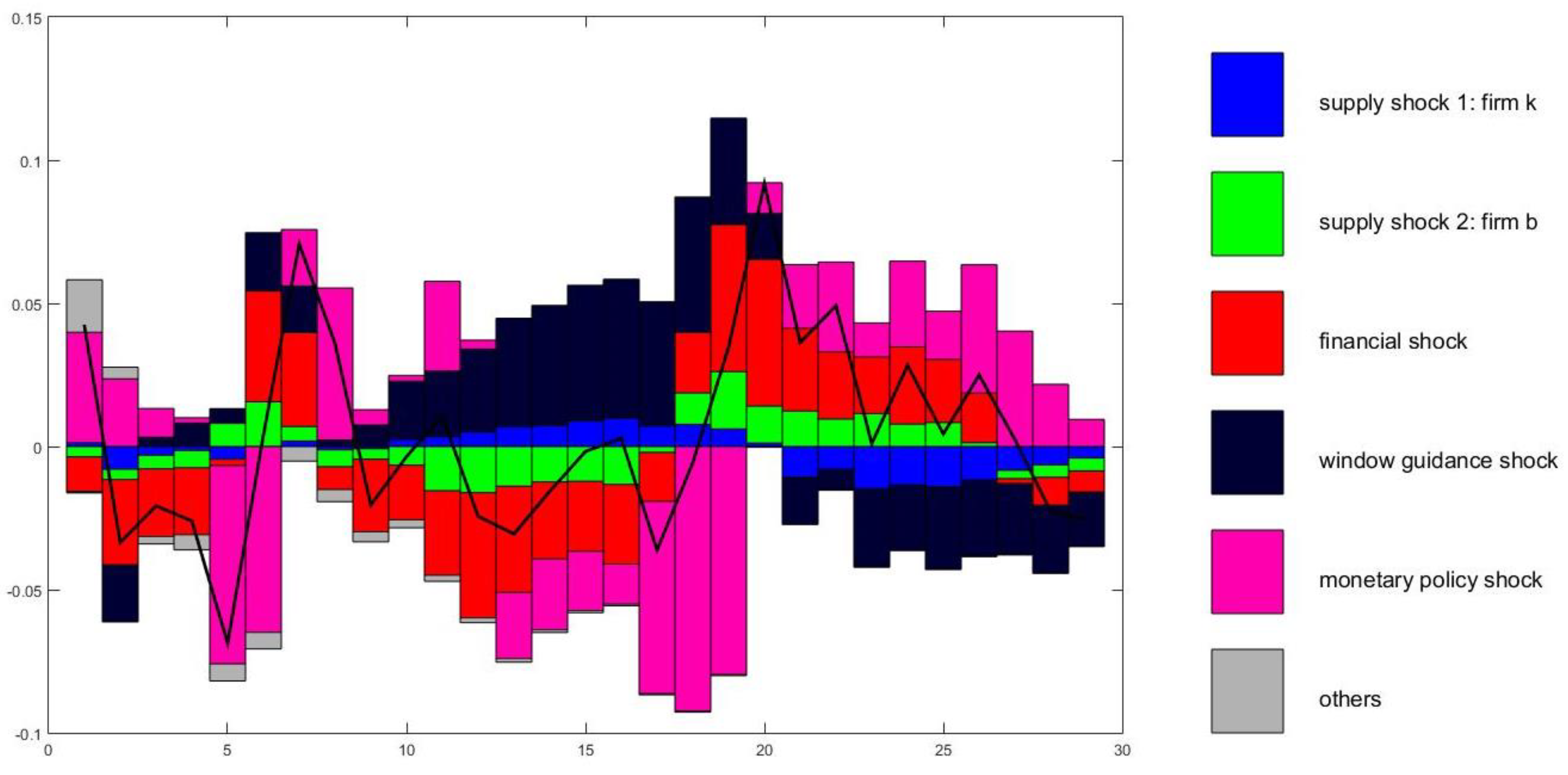
From Figure 4, it can be seen that financial market shock and monetary policy shock greatly impacts on the rate of return of financial assets. Specifically, Figure 4 depicts the following information. The volatility in financial asset yield rate is opposite to the volatility in financial market impact. It can be inferred from the basic knowledge of finance that a positive financial shock causes the price of financial assets to rise, which is equivalent to reducing the rate of return of financial assets. Therefore, it is not difficult to understand why the above two fluctuate with opposite trends. Second, in each period, monetary policy shocks are almost the opposite of financial market shocks. This is an interesting phenomenon. The occurrence of this situation reflects the characteristic of monetary policy to lean against the wind. When financial markets encounter positive external shocks, the rise in financial asset prices will cause the bank to transfer credit funds to financial assets. In order to curb overheated financial markets, monetary policy makers working on counter-cyclical regulation will tighten monetary policy and reduce the supply of credit. As such, commercial banks find that there are no available funds to invest in the financial market, thus inhibiting the supply of funds and preventing the emergence of financial market bubbles.

Figure 5 shows the historical variance decomposition of the ratio of credit assets to financial assets. First, financial shocks lead to fluctuations in the ratio of credit assets to financial assets. Second, the volatility is almost consistent with the monetary policy shock, meaning the negative monetary policy shock is accompanied by the decline in the proportion of credit assets and financial assets in the same period. From the previous analysis, the negative monetary policy curbs the flow of credit funds to financial markets, i.e., the negative monetary policy curbs the decline of $x_t$. Therefore, it is not difficult to understand why there is a positive correlation among these two variables, suggesting that tighter monetary policy has not fully suppressed the decline of $x_t$.

Figure 6 depicts the historical variance decomposition of the ratio of financial assets to bank net worth ${\psi }_t$. First, the leverage ratio of financial assets and financial shock change synperiodically. The negative financial shock reduces the price of financial assets, which reduces the bank’s allocation of financial assets. Second, in recent years, China’s monetary policy has shown a structural characteristic. Specifically, in the same period, monetary policy shocks and window guidance shocks move inversely with each other. Besides tightening monetary policy by increasing the monetary policy rate, the central bank reduces the lending rate of credit funds, which guarantees that SME financing costs are unchanged.

5.3. Financial Shock

Figure 7 simulates the impact of financial market volatility on the macro economy. A 1% negative volatility shock in the financial market immediately lead to a fall in the price of financial assets $Q_t$. The financial market recession leads to an increase in various interest rate indicators, including benchmark interest rates and financial asset yields. However, the return on financial assets that are more closely linked to the financial market will be more intense, leading to an increase in spreads $R_k-R_b$. Simultaneously, the decline in financial assets price causes banks to reduce their holdings of financial assets. $S_t$ also declines.

Along with the sudden loss of the bank’s financial assets, the bank’s net asset value $n_t$ also fall. Due to the leverage ratio between financial assets and the bank’s net assets, the decline in the value of the bank’s net assets will be even greater, reaching around 7%. The reduction in the value of the bank’s net assets leads to a contraction in the issuance of credit assets through leverage within the banking system. Once again, due to the leverage ratio within the banking system, the size of credit assets falls by around 5%. Therefore, in terms of the total amount, the scale of credit assets and financial assets declines due to financial market volatility and the depreciation of the bank’s net assets.

Because financial market volatility reduces the income of financial assets, financial assets are no longer strongly attractive to banks. At this time, the stable and safer characteristics of credit asset income causes banks to allocate more capital to credit assets on the asset side, resulting in an increase in the ratio of credit assets to financial assets $x_t$. Therefore, in terms of proportion, the decline in the size of financial assets is more obvious than the shrinking of credit assets.

According to our model, direct financing producers are financed by issuing marketable interests in financial markets, and indirect financing producers are financed through bank credit. Fluctuations in the financial market affect the production scale of both types of production enterprises. The impact on direct financing producers is more obvious. As can be seen from the impulse response graph (Figure 8), the output of direct financing firms falls by about 4%, while the output of indirect financing producers falls by about 1.5%. The decline in output of the two types of production companies ultimately leads to a decline in total social output.

The decline in asset prices causes the bank’s assets to contract, which in turn leads to a contraction of the debt side, thereby reducing the return on household savings. A reduction in the production scale of a production enterprise reduces labor employment, and the labor compensation received by the family decreases. In short, the total income of the family decreases, and thus the total consumption decreases.

Depicted in the impulse response graph, the volatility shock from the financial market first affects the yield of financial assets, and then affects the holding ratio of financial assets and credit assets. This has an asymmetric impact on the production scale of the two types of production enterprises. The endogenous changes in the leverage of the banking sector caused by the exogenous impact of the financial market will eventually have a magnifying effect on economic fluctuations.

5.4. Monetary Policy Shocks

Figure 8 depicts the impact of a 1% tightening monetary policy shock on key macroeconomic variables. The impulse response graph shows that tight monetary policy curbed social demand such as consumption and investment, with the two falling by 2.4% and 0.7% respectively, and the total social output also falling, with the total output falling by 1.8%.

First, tightening monetary policy impacts the financial sector. Tightening monetary policy will raise interest rates. However, since financial markets are less constrained and regulated than traditional credit markets, interest rates in various markets are not exactly the same. Specifically, in the financial market, asset prices fall by nearly 0.3% and the yield of financial assets rise sharply. Compared with credit interest rates, the spread of financial assets rises by more than 0.2%. The decline in the yield of financial assets directly causes banks to reduce the amount of financial assets held by their banks, and the decline in holdings is about 5%. Because the yields of both credit assets and financial assets are different, the reduction in the total size of the two types of assets is also different, and financial assets shrink more significantly. Therefore, the ratio of the two rise relatively, with an increase of about 4%. At the same time, the decline in the price of financial assets leads to a reduction in bank profits, and the bank’s net assets also decline. With economic downturn, banks are generally no longer optimistic about the financial market and reduce the leverage ratio of financial assets. The current period ${\psi }_t$ also declines by about 0.25.

Second, the upward trend in interest rates leads to an increase in investment costs and a decrease in entrepreneurs’ willingness to invest. Along with the contraction of various financing markets, the corresponding production companies also reduce their production scale. Producers financed through financial assets are more affected, with production falling by about 2%. The output of producers financed through credit also falls by about 1.5%. In short, the scale of production of the entire society declines. The reduction in total social supply causes an increase in prices, and the inflation rate increases by about 0.9%.

Notably, consumption shows a decreasing trend, by about 2.4%. We think that there are two reasons for this phenomenon. Firstly, the rise in interest rates may increase the return on savings, and people are more willing to save money than consume, which leads to a reduction in consumption. Secondly, the reduction in total social supply also reduces the total amount of products available for consumption, which also inhibits the total social demand to some extent.

6. Conclusions

Due to the unique interest rate dual-track system, the deposit and loan interest rates of the traditional bank credit business are subject to more government regulation. The yields of securities circulating in the financial market, such as bonds, can fluctuate with market fluctuations, and are less constrained by the government, which can reflect the macroeconomic environment more realistically. Accordingly, we divided the assets held by China’s commercial banks into credit assets and financial assets. The model includes two types of productive enterprises: direct financing and indirect financing. The former are financed by issuing financial assets in the market, and the latter are financed through bank credit assets. By constructing a DSGE model containing a bank’s balance sheet, we characterized the impact of different exogenous shocks on macroeconomics through the bank’s balance sheet channel.

The results of the impulse response show that the negative impact from the financial market will shrink the size of both types of assets. However, the return on credit assets is regulated by the government and the scale is limited, resulting in different contraction ratios for the two types of assets. Furthermore, the production scale of the two types of productive enterprises also shows an asymmetric contraction. A shock from the supply side will cause the price of financial assets to rise, and the spread of the two types of assets will shrink. Moreover, the size of both types of assets expands at the same time. The impact from tight monetary policy leads to an increase in the yields of various assets, and the scales of various assets shrink. Loan interest rates controlled by the government increase less than the yield of financial assets, so the spread of the two types of assets expands, and the banks allocate more assets to the credit assets. This results in a relative increase in the proportion of credit assets and the asymmetric contraction of the two type enterprises production scale, that is, the decline in the output of direct financing enterprises is more obvious.

Based on the existing literature, this paper expands the single-type assets held by banks into two types of assets with different characteristics, and explains the economic fluctuations in China from the perspective of bank assets, thus providing a new perspective for understanding of China’s macroeconomic fluctuations.

References

- Angeloni, Ignazio, and Ester Faia. 2013. Capital regulation and monetary policy with fragile banks. Journal of Monetary Economics 60: 311–24. [Google Scholar] [CrossRef]
- Canova, Fabio. 1998. Detrending and business cycle facts: A user’s guide. Journal of Monetary Economics 41: 475–512. [Google Scholar] [CrossRef]
- Chen, Xiaoguang, and Yulin Zhang. 2010. Credit Constraint, Government Consumption and China’s Actual Economic Cycle. Economic Research 45: 48–59. [Google Scholar]
- Chen, Xin, Huaming Wang, and Yuchao Peng. 2017. The Causes of Social Financing Scale Fluctuation and Its Reflection on Macroeconomics—Based on DSGE Model and Its Variance Decomposition Analysis. Investment Research 36: 36–51. [Google Scholar]
- Chun, Chang, Kaiji Chen, Daniel F. Waggoner, and Tao Zha. 2015. Trends and Cycles in China’s Macroeconomy. Working paper. Atlanta: Federal Reserve Bank of Atlanta. [Google Scholar]
- Dib, Ali. 2009. Credit and Interbank Bank Markets in a New Keynesian Model. Mimeo: Bank of Canada. [Google Scholar]
- Du, Qingyuan, and Liutang Gong. 2005. A RBC Model with Financial Accelerator. Journal of Finance 4: 16–30. [Google Scholar]
- Gertler, Mark, and Peter Karadi. 2011. A model of unconventional monetary policy. Journal of Monetary Economics 58: 17–34. [Google Scholar] [CrossRef] [Green Version]
- Gertler, Mark, and Nobuhiro Kiyotaki. 2010. Financial Intermediation and Credit Policy in Business Cycle Analysis. In Handbook of Monetary Economics. Edited by Benjamin M. Friedman and Woodford Michael. Amsterdam: Elsevier. [Google Scholar]
- Gertler, Mark, Nobuhiro Kiyotaki, and Albert Queralto. 2012. Financial crises, bank risk exposure and government financial policy. Journal of Monetary Economics 59: S17–34. [Google Scholar] [CrossRef]
- Goodfriend, Marvin, and Bennett T. McCallum. 2007. Banking and interest rates in monetary policy analysis: A quantitative exploration. Journal of Monetary Economics 54: 1480–507. [Google Scholar] [CrossRef]
- Iacoviello, Matteo. 2005. House Prices, Borrowing Constraints, and Monetary Policy in the Business Cycle. American Economic Review 95: 739–64. [Google Scholar] [CrossRef]
- International Monetary Fund (IMF). 2008. Global Financial Stability Report: Market Development and Issues. Beijing: China Financial Publishing House. [Google Scholar]
- Kang, Li, and Liutang Gong. 2014. Financial Friction, Bank Net Assets and International Economic Crisis Transmission—Based on Multi-sector DSGE Model Analysis. Economic Research 49: 147–59. [Google Scholar]
- Li, Daokui, and Mei Song. 2009. The US dollar M_2 contraction induced the world financial crisis: The internal and external factors of the financial crisis and its test. World Economy 4: 15–26. [Google Scholar]
- Liu, Xiaoxing, and Dengbao Yao. 2016. Financial Disintermediation, Asset Price and Economic Fluctuation: Based on DNK-DSGE Model Analysis. The Journal of World Economy 39: 29–53. [Google Scholar]
- Lv, Zhaofeng, and Meibo Huang. 2011. Analysis of China’s economic cycle welfare cost. The Journal of World Economy 6: 71–83. [Google Scholar]
- Meh, Césaire A., and Kevin Moran. 2010. The role of bank capital in the propagation of shocks. Journal of Economic Dynamics & Control 34: 555–76. [Google Scholar]
- Mei, Dongzhou, and Liutang Gong. 2011. The Determinants of Exchange Rate Regime in the Emerging Economies. Economic Research Journal 11: 74–86. [Google Scholar]
- Ming, Ming, Licong Zhang, and Jingwei Yu. 2017. Commercial Banking and Bond Market: Looking at Interest Rate Changes from Subjects. Interest Rate Debt Weekly 10: 7–20. [Google Scholar]
- Nelson, Charles R., and Charles R. Plosser. 1982. Trends and random walks in macroeconomic time series: Some evidence and implications. Journal of Monetary Economics 10: 139–62. [Google Scholar] [CrossRef]
- Qiu, Xiang, and Qianglong Zhou. 2014. Transmission of shadow banking and monetary policy. Economic Research 49: 91–105. [Google Scholar]
- Shan, Haojie. 2008. Reestimating the Capital Stock of China: 1952–2006. The Journal of Quantitative & Technical Economics 10: 17–32. [Google Scholar]
- Sun, Xiaotao. 2013. The Cycle of Trend Decomposition Theory and Chinese Economy. Ph.D. Thesis, Huazhong University of Science and Technology, Wuhan, China. [Google Scholar]
- Tang, Xiaobin, and Jinquan Liu. 2012. Correlation Analysis between Inflation, Uncertainty of Inflation and Uncertainty of Money Growth. Systems Engineering 5: 17–23. [Google Scholar]
- Wang, Qing, and Jiao Tian. 2016. Bank Capital Supervision and Systematic Financial Risk Transfer—Analysis Based on DSGE Model. China Social Sciences 3: 99–122. [Google Scholar]
- Yan, Chaoming. 2008. The Great Recession: How to Survive and Develop in the Financial Crisis: Lessons from Japan’s Great Recession. Pune: Oriental Publishing House. [Google Scholar]
- Yi, Huiman. 2017. Reconstructing the bank’s balance sheet. China Finance 1: 9–13. [Google Scholar]
- Zheng, Chao. 2016. The Operation Mode and Development Strategy of China’s Commercial Banks’ Investment and Loan Linkage. Southern Finance 6: 20–25. [Google Scholar]
- Zhuang, Ziguan, Xiaoyong Cui, Liutang Gong, and Hengfu Zou. 2012. Expectations and Business Cycle: Can News Shocks Be a Major Source of China’ s Economic Fluctuations? Economic Research Journal 6: 46–59. [Google Scholar]
Figure 1.
The trend of assets of commercial banks. (Data sources: Wind).
Figure 2.
The proportion of traditional credit in social aggregate financing. (Data source: Wind).
Figure 3.
Theoretical model framework.
Figure 4.
Historical decomposition of the return rate of financial assets based on the posterior mean estimates of parameters and the Kalman smoothed mean estimates of shock. The y-axis represents the percentage point deviation from steady state. The full line represents the , which means the deviation from steady state value of . The following figures are similar.
Figure 5.
The historical variance decomposition of the ratio of credit assets to financial assets .
Figure 6.
The historical variance decomposition of the ratio of financial assets to bank net worth .
Figure 7.
Impulse response diagram of financial market shock.
Figure 8.
Impulse response diagram of monetary policy shock.