Machine Learning-Based App for Self-Evaluation of Teacher-Specific Instructional Style and Tools


1
School of Physical and Mathematical Sciences, Nanyang Technological University, SPMS-MAS-05-23, 21 Nanyang Link, Singapore 637371, Singapore
2
School of Physical and Mathematical Sciences, Nanyang Technological University, SPMS-MAS-04-10, 21 Nanyang Link, Singapore 637371, Singapore
*
Author to whom correspondence should be addressed.
Educ. Sci. 2018, 8(1), 7; https://doi.org/10.3390/educsci8010007
Submission received: 27 September 2017
/
Revised: 31 December 2017
/
Accepted: 3 January 2018
/
Published: 10 January 2018
(This article belongs to the Special Issue Collaborative Learning with Technology—Frontiers and Evidence)
Abstract
:Course instructors need to assess the efficacy of their teaching methods, but experiments in education are seldom politically, administratively, or ethically feasible. Quasi-experimental tools, on the other hand, are often problematic, as they are typically too complicated to be of widespread use to educators and may suffer from selection bias occurring due to confounding variables such as students’ prior knowledge. We developed a machine learning algorithm that accounts for students’ prior knowledge. Our algorithm is based on symbolic regression that uses non-experimental data on previous scores collected by the university as input. It can predict 60–70 percent of variation in students’ exam scores. Applying our algorithm to evaluate the impact of teaching methods in an ordinary differential equations class, we found that clickers were a more effective teaching strategy as compared to traditional handwritten homework; however, online homework with immediate feedback was found to be even more effective than clickers. The novelty of our findings is in the method (machine learning-based analysis of non-experimental data) and in the fact that we compare the effectiveness of clickers and handwritten homework in teaching undergraduate mathematics. Evaluating the methods used in a calculus class, we found that active team work seemed to be more beneficial for students than individual work. Our algorithm has been integrated into an app that we are sharing with the educational community, so it can be used by practitioners without advanced methodological training.
1. Introduction
There exists a gap between educational research and teaching practice. Indeed, according to John Hattie, the author of [1]—a synthesis of more than 800 meta-studies:
We have a rich educational research base, but rarely is it used by teachers, and rarely does it lead to policy changes that affect the nature of teaching.
One of the reasons is perhaps that, according to William E. Becker (see [2]),
Quantitative studies of the effects of one teaching method versus another are either not cited or are few in number.
There are reasons why trustworthy quantitative studies are scarce in education. The gold standard of a quantitative study is a randomized controlled trial. Proper randomized clinical trials are seldom available in the classroom because educators are given resources to teach rather than to conduct experiments on students. When a randomized trial is beyond the bounds of possibility, researchers resort to quasi-experiments. Quasi-experiments are often plagued by selection bias caused by unobserved or confounding variables such as students’ diligence, talent, motivation, pre-knowledge, personal affection for the course instructor, headache on the exam day, etc. For example, if students have an option to use clickers in class, then students who consciously choose to do so are likely to get higher exam scores than students who do not, not mainly because of the pedagogical benefits of using clickers, but simply because the former were more diligent to begin with. In order to evaluate the efficacy of clickers, diligence needs to be controlled for. As another example, students from a hypothetical tutorial group 1 may get higher exam scores than students from tutorial group 10 not because they had a better teacher but rather because tutorial group 1 was formed of students who matriculated earlier; the main reason for their early matriculation being early admission due to the fact that the university saw them as talented. In order to compare results in tutorial groups 1 and 10, students’ talent needs to be controlled for.
Unlike drugs that often have harmful side effects, teaching methods are almost always beneficial for learning (see, again, [1]—John Hattie’s synthesis of more than 800 meta-studies). The meaningful question for an education researcher is therefore not whether a teaching method helps students to learn (it most likely does), but rather if one teaching method works better than another. As an example, consider an intelligent tutoring system such as MyMathLab from Pearson Education [3], which grades calculus exercises and gives students feedback on their progress. Solving exercises in such an intelligent tutoring system is very unlikely to be detrimental. However, whether the intelligent tutoring system is more effective than a human tutor and whether it is worth the money invested is a question of high practical interest.
An educator often needs to evaluate an instructional tool rather than a particular teaching method, approach, or strategy. Unlike a drug that is either administered or not administered, an instructional tool often admits a multitude of practices. An example of such a versatile instructional tool is a round table or, rather, re-furnishing tutorial rooms with round tables for team activities. The practical question for an instructor is how to organize team activities. Doing it right is clearly a challenging task. To begin with, the instructor needs to decide whether teams should be consistent throughout the whole semester (such as in [4]), or occasionally randomized (as in [5]). The answer depends on factors such as the discipline taught, intended learning outcomes, students’ cultural background, etc. Sometimes, the solution may be to try both consistent teams and teams that are being reshuffled and see what works best for students in the particular class.
A number of authors have developed machine learning algorithms to assist educators. The central theme of this research is predicting students’ performance—see, for example, [6]. There exist prototypes of software for predicting students’ performance [7]. The main motivation is usually to identify students who have a high chance of dropping out or are at risk of failing the course, and help them by an early intervention. The challenge is improving the accuracy, sensitivity, and specificity of the machine learning algorithms. The predictive model of students’ performance is therefore trained on early stages of the course’s progress for the educator to have ample time for the intervention.
In this paper, we propose a novel application of machine learning for the purpose of controlling for confounding variables in quasi-experiments in education. We argue that much of the confounding is contributed by variables such as pre-knowledge, diligence, and talent. As an example, let us think of a first semester undergraduate course in mechanics whose prerequisites are high school calculus and high school physics. If we know students’ high school grades, then pre-knowledge and talent in calculus and physics are measured by grades in the respective subjects, and diligence is measured by the average high school grade. Now, if we build a machine learning algorithm for predicting exam scores in mechanics based on high school grade point average and high school grades in calculus and physics, then much of confounding will be controlled for. Such a predictive model is trained after the course has ended with the purpose of improving it the next time the course is offered.
It is important to note that actual exam scores are not linear functions of other exam and test scores [8], and they do not follow some other simple well-defined form (e.g., logistic, probit, power law, log-linear, etc.). Because of that, we do not use classical regression models based on specific assumptions about the model. Other popular machine learning algorithms (random forests, artificial neural networks, support vector machines), while being able to attain remarkable precision, often produce non human-interpretable results. We have chosen a machine learning algorithm that produces explicit human-interpretable models and yet does not assume any specific form in advance—symbolic regression [9].
Our research problem is the development of a methodology and a practical tool for assisting in quasi-experiments in education. The methodology is unsophisticated. The practical tool is a user-friendly app tailored for educators who may not be familiar with elaborate experimental designs based on advanced statistical techniques. The main source of data is non-experimental data. Specifically, we hope to show how a course instructor can teach a course as per normal while still being able to analyse data on students’ scores and extract meaningful and actionable insights on the efficacy of their teaching methods from data on students’ scores which are automatically collected by the university.
Our methodology of controlling for confounding variables by a machine learning algorithm is not meant to replace randomized controlled trials or classical quasi-experiments. However, when a proper randomized trial or a classical quasi-experiment are not available (e.g., if the course instructor is not familiar with relevant statistical techniques or is simply too busy teaching) and the course instructor has to make a judgment on which teaching methods worked best in their class, judgement based on research literature, pedagogical expertise, and data analysis is more credible than judgement based solely on research literature and pedagogical expertise. We argue that with the help of our app, data analysis will be manageable.
Our methodology and our app can be useful for institutions. A retrospective example is the university the authors work in. A few years ago, our university bought clickers for all undergraduate students. The decision to invest in clickers was based on the fact that, according to large studies such as [10,11], active learning is more effective than traditional didactic teaching. The technology was given a trial run for a few semesters. Instructors and students participating in the trial run gave an overall positive feedback on the technology. However, this feedback was based on opinions and was therefore subjective. Had our app been available then, instructors participating in the trial run would have been able to support their feedback with hard data. With hard data on how clickers (a particular tool associated with active learning) helped students at the particular university to improve their performance, outcomes of the clickers endeavour may have been different.
2. Methodology
Selection bias in educational quasi-experiments occurs due to a variety of confounding variables, such as students’ diligence, talent, motivation, pre-knowledge, personal affection for the course instructor, headache on the exam day, etc. Much of the confounding can be accounted for by scores in a diagnostic test and by previous grades. While previous grades do not measure diligence and talent directly, it is still reasonable to expect that talent and diligence affect previous grades in similar subjects in the same way as they do the experimental subject. If a student has been getting high grades in mathematics, she is likely to be mathematically gifted and hence is expected to continue getting high grades in mathematics. A student with a high cumulative grade point average (CGPA) is likely to be diligent, and hence she is expected to get high grades in all subjects. While measuring pre-knowledge carefully and precisely will require thorough testing, even a simple diagnostic test will reflect true pre-knowledge to a certain extent.
Scores in a diagnostic test and previous grades are non-experimental data (i.e., data that are automatically collected by the university). Course instructors usually have direct access to all students’ results in their experimental course; grades from previous courses can be obtained via the relevant authority (in our case, it was the Student Affairs Office). The latter will require some negotiating with the management, but it is doable since
- Exam scores are automatically collected and stored;
- Data on exam scores can (and should) be easily anonymized;
- The purpose of research is to identify teaching methods that work best for a particular instructor (i.e., improve teaching and learning);
- Data on previous grades will be requested for and merged with data on current students’ results only after the course is over, thereby excluding personal biases the instructor may otherwise acquire.
We call the collection of results in a diagnostic test and grades from previous courses a student’s initial level of preparation, and we argue that the initial level of preparation contains a great deal of information about unobservable confounding variables—pre-knowledge, talent, and diligence. After the experimental course is over, a predictive model is constructed to predict students’ results in the experimental course from their initial level of preparation. As a hypothetical example, let us think of a course in Analytical Chemistry (ACHEM). Suppose that the course instructor conducted a diagnostic test (DTest) and, after Analytical Chemistry was graded, acquired his students’ grades in Basic Inorganic Chemistry (ICHEM) and Basic Physical Chemistry (PCHEM)—pre-requisites to Analytical Chemistry. Table 1 contains the scores of four hypothetical students and the predicted score (Pred) out of a maximum of 100.
Note that Alice has the highest score in the experimental subject, but this is explained by the fact that she was expected to succeed. If she was exposed to experimental treatment, her high score in the course is most likely not due to experimental treatment, but rather because she was a stronger student to begin with. Diane was a weak student and hence she was expected to get a low score in the course. As for Brian and Cortney, their true scores are remarkably different from the model’s predictions. Brian over-performed the model by 11 points and Cortney underperformed the model by 11 points. Figuratively speaking, Brian here is the true winner and Cortney is the true loser.
Let the Added Value be the residual of the model, i.e.,
For instance, in the example above. Thus, Added Value is the course score controlled for the initial level of preparation. A large positive Added Value indicates that the student’s result is higher than that of students with similar initial level of preparation. A large negative Added Value shows that the student’s result is lower than that of students with similar level of preparation. Figuratively speaking, Added Value is the true measure of success in a course.
Constructing a predictive model (i.e., calculating the numbers in the column “Pred” above) is the task of supervised machine learning. A great number of machine learning algorithms are known. The interested reader can be referred to [12] or to any other textbook on machine learning or data mining. Each algorithm for machine learning has its own limitations that are important for choosing the right algorithm for our purpose; i.e., for controlling for the initial level of preparation in educational quasi-experiments. Considerations of educational quasi-experiments are:
- Each entry in the data set represents a student registered for the course, and hence data sets may be (and usually are) small. This rules out algorithms that require massive training data sets, such as artificial neural networks.
- Educational data sets have missing entries—imagine a student who was sick on the day of the diagnostic test. Dealing with missing data is an issue with some popular algorithms, such as support vector machines.
- Machine learning algorithms are often prone to overfitting, and this is an especially pressing issue when data sets are small. This rules out some algorithms, such as random forests.
- We do not know what the form of the predictive model should be. This rules out classical statistical models, such as linear regression, logistic regression, probit regression, log-log linear regression, Poisson regression, etc.
- Machine learning algorithms may or may not do feature selection; i.e., identify independent variables that are important for predicting, ruling out those that are not, and dealing with highly correlated predictors. In an educational setting, feature selection, although not vital, would be very useful. This rules out algorithms such as the k-nearest neighbours.
Note that the scenario that we have in mind is course instructors constructing and interpreting predictive models. Therefore, some issues that may not be seen as serious challenges by machine learning experts—such as overfitting and dealing with missing data—are actually very important considerations.
Upon carefully weighing the pros and cons of machine learning algorithms, we decided to choose symbolic regression. Models produced by symbolic regression are explicit equations in terms of predictors. For instance, a possible equation for our hypothetical example of Analytical Chemistry may be
Since the model is transparent, we can examine it and notice that it does not include PCHEM, it is an increasing function of DTest and ICHEM for feasible values of both predictors (i.e., between 0 and 100), and that it is practically independent of DTest for . These observations may be important in practice to validate the model.
Symbolic regression is an evolutionary algorithm. It first generates some models at random and then starts (metaphorically speaking) breeding them, so those that fit the data best survive and produce offspring—more models that continue to evolve. The output of symbolic regression is visualized as a scatter plot, such as the one shown in Figure 1. Each model is represented by a dot on the plane complexity–error. Models that are on the far right of the diagram are too complex, and hence they may overfit. Models that are on the top left of the diagram are too imprecise. Models that are unsurpassed by either precision or complexity form the so-called Pareto front—red dots in Figure 1. Models in the bottom left corner of the diagram are those with optimal combination of precision and complexity—they are not too complex and yet are precise. In Figure 1, for models that are in the bottom left of the diagram is between and ; i.e., R (linear correlation between the model’s prediction and true results) is between and —that is, these models account for between 70% and 73% of the variation in exam scores).
The algorithm will then form a model ensemble—a small subset of models in the bottom left corner of the diagram. To calculate the predicted value, one simply takes the median of the model ensemble. Variables that actually occur in models selected for the model ensemble are important for predicting; variables that do not occur in the model ensemble are not important for predicting. If the data set contains missing values, models including these variables will not predict anything, and the whole ensemble may not predict anything for that particular student.
Several implementations of symbolic regression are known. We have chosen DataModeler— an add-on to Wolfram Mathematica—for our work. The reader interested in technical specifications of DataModeler is referred to [13]. The advantage of DataModeler is that it is a professional package for industrial tasks. The disadvantage is that it is a proprietary software built on top of another proprietary software (i.e., in order to use our app for educational data mining, educators will have to buy a license for Wolfram Mathematica and a license for DataModeler, even though the app itself is free of charge). We hope that the burden is not too heavy, since many universities have a few Mathematica licenses and since developers of DataModeler allow the installation of a 60-day free trial version.
3. Quasi-Experiments
Although we are using the word “quasi-experiments”, data used for them are non-experimental data of students’ scores collected by the university. As instructors, we have direct access to a large portion of these data. We have access to students’ scores in a pre-test, students scores for course activities, and students’ scores for the main assessment (final exam or a project). We obtained students’ grades in previous courses from the Student Affairs Office. All the data are non-experimental in the sense that they are routinely generated throughout the normal process of teaching and learning. The data would be collected and stored by the university with or without our quasi-experiments.
Quasi-experiment 1 was conducted in 2015 and 2016 by the first author teaching ordinary differential equations. Teaching methods involved clickers, handwritten homework, and online homework. Data collected in 2015 showed that handwritten homework was not an effective teaching method as compared to clickers. Based on data analysis, the first author decided to replace handwritten homework with online homework in 2016, the next time the course was taught. Data collected in 2016 showed that online homework was a more effective method that clickers.
We set the level of statistical significance to be . The level is large because our method is designed for processing noisy non-experimental data, and results are meant to help the course instructor to make a decision on which teaching methods work best in a particular course rather than to make far-reaching conclusions on what works for all students across disciplines, ages, and cultures.
With , we cannot reject the null hypothesis that the median added value for students who preferred clickers to handwritten homework is the same as that for students who preferred homework to clickers (p-value of the u-test was above ). However, we reject the null hypothesis that the mean added value for students who preferred clickers to handwritten homework in 2015 is the same as that for students who preferred homework to clickers (p-value of the t-test is below ). The finding that the mean and the median added value for students who preferred online homework to clickers in 2016 is not statistically significant. The reader interested in further details on statistical tests and regression analysis is referred to the supplementary materials.
Quasi-experiment 2 was conducted in 2016 by the second author teaching first year calculus. The course design was Team-Based Learning (see [4] for an overview of the Team-Based Learning Pedagogy). The main purpose of Quasi-experiment 2 is to test whether team work or individual work is more beneficial to students. It was found that team work was more beneficial in the sense that students who got high scores for team work also ended up with higher exam scores than scores predicted given their initial level of preparation. Students who got high scores for individual work ended up with approximately similar exam scores as scores predicted given their initial level of preparation. It is not immediately clear whether the findings of Quasi-experiment 2 have any practical application, but Quasi-experiment 2 still demonstrates our approach to educational quasi-experiments.
3.1. Quasi-Experiment 1
The first author taught an ordinary differential equations course in 2015 and 2016. In both cases, students could choose between two learning activities—clickers and homework. To get the full score for the learning activities, they needed to have solved more than a certain number of exercises of either type. They could invest all their effort into homework and occasionally attend clicker sessions, or they could invest all their effort into clicker sessions and do homework occasionally, or they could try an even mixture of homework and clickers. In both cases, clicker sessions were early in the morning and, presumably, low-motivated students preferred homework. Most students had not been previously exposed to clickers but had been familiar to homework since childhood. Students were encouraged but not forced to collaborate on both activities. Either homework or clicker questions covered about 70% of material that later appeared in the final exam, but students did not know this in advance.
The main difference between 2015 and 2016 is that in 2015 students submitted handwritten homework and received feedback from tutors within approximately 2 weeks after the lecture, while in 2016 students were allowed (but not forced) to submit homework as a shared online LaTeX document [14]. Those who submitted homework as a shared online LaTeX document received feedback within hours and were allowed to re-submit their work based on feedback received. The majority of 2016 students preferred submitting homework online to get unlimited attempts, even though they often complained about having to learn LaTeX. Another difference is that each clicker session lasted for 2 h in 2015 but only for 1 h in 2016, and the number of questions in 2016 was 60% of the number of questions in 2015. Table 2 summarizes the similarities and differences between learning activities in 2015 and 2016. One more difference not reflected in Table 2 is that in 2015, the final exam was 52% of the total course mark, while in 2016 the final exam was 35%. There was also a team project in 2016.
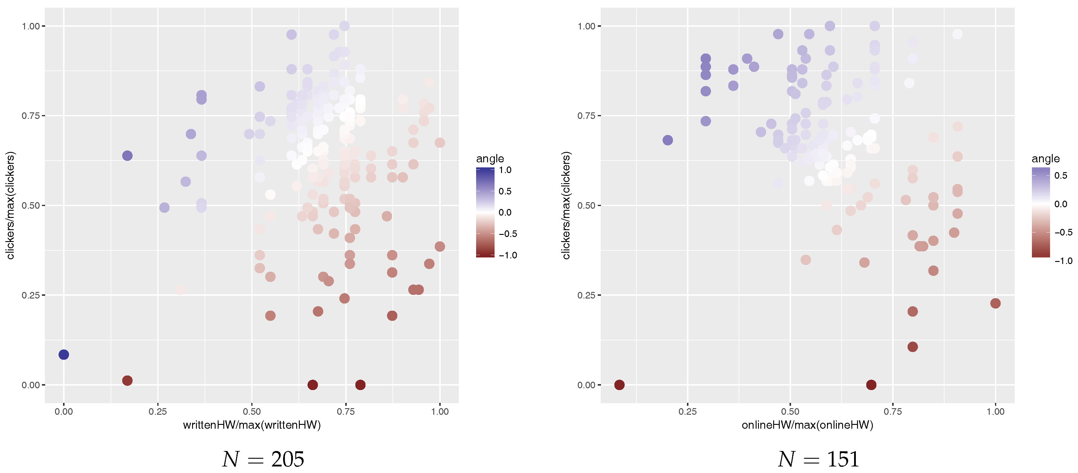
Figure 2 shows students’ preference towards clickers or homework in 2015 and 2016. Each point in Figure 2 represents a student. The x-axis is the normalized homework score and the y-axis is the normalized clicker score; normalization was done by dividing by the sample maximum. The colour of points represents preference towards clickers or homework (red for homework and blue for clickers).
In both 2015 and 2016, we acquired students’ exam grades in Calculus 1, Calculus 2, Calculus 3, Linear Algebra 1, and Linear Algebra 2, since these subjects contain material which is important for the theory of differential equations. Table 3 contains a sample of 2015 raw data and Table 4 contains a sample of 2016 raw data. Note that in both cases we rescaled all exam scores so that the maximum is 100 and the minimum is 0; we did this so that true exam scores of our students would not be revealed, even though they have been anonymized.
In both 2015 and 2016, we constructed predictive models to predict the exam score from previous grades in Calculus 1, Calculus 2, Calculus 3, Linear Algebra 1, and Linear Algebra 2. These predictive models are shown in Figure 3. In both cases, the error of the models was approximately (i.e., ). This means that our models account for more than 70% in exam score variation.
In order to compare teaching methods, we identified a group of students who preferred clickers to homework and a group of students who preferred homework to clickers. This was done as follows: for each student, we computed the ratio
and then top 10% (i.e., 21 students in 2015 and 15 students in 2016) of students with the highest ratio are those who prefer clickers to homework and the bottom 10% (again, 21 students in 2015 and 15 students in 2016) are those who prefer homework to clickers. This ratio is visualized as colours of points in Figure 2, blue—high (preference towards clickers), white—about 1 (neutral), red—low (preference towards homework).
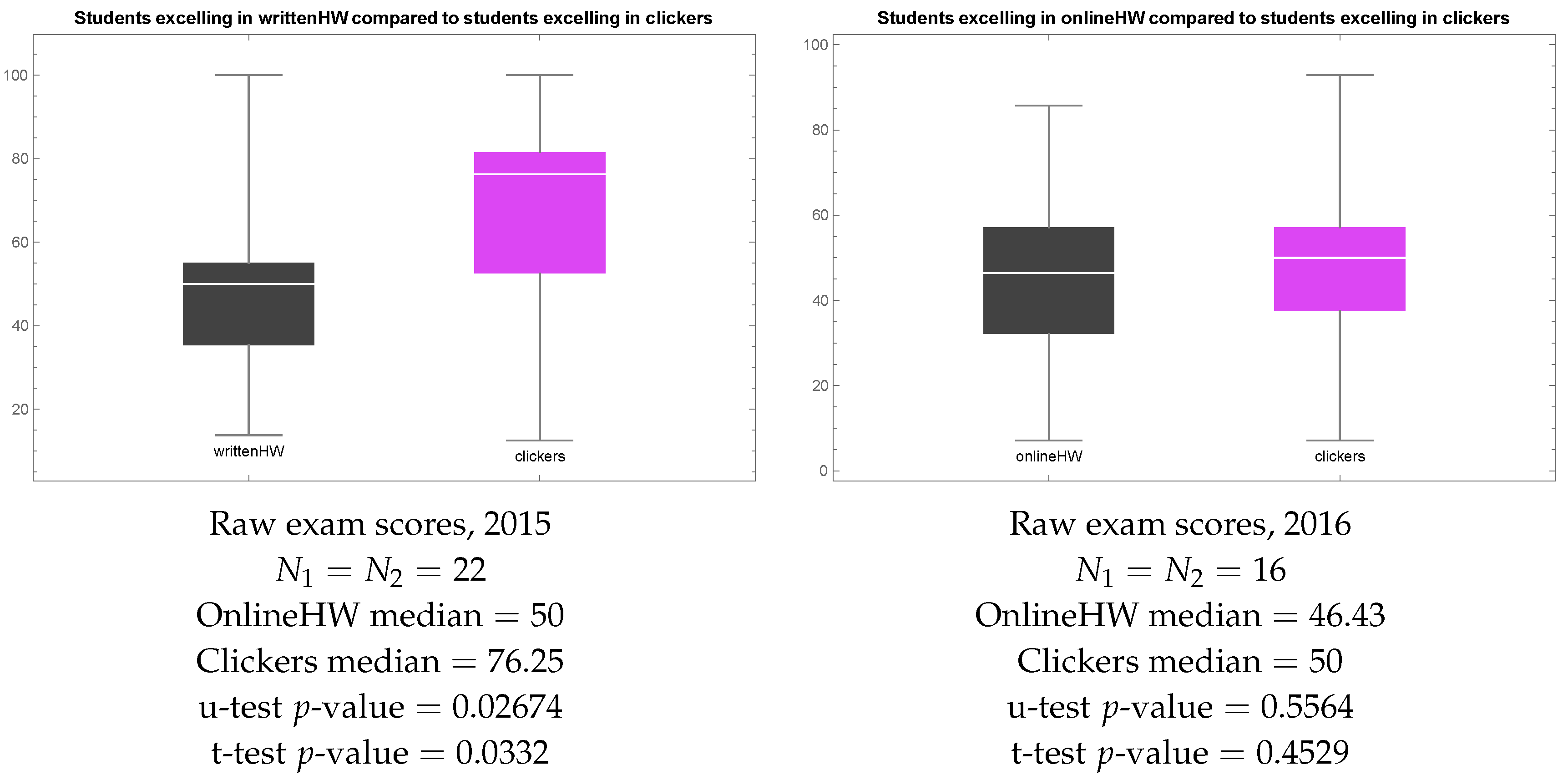
Further, we visualized raw exam scores in 2015 and 2016 in each of the two groups as box plots—Figure 4. The box plot shows the minimum, 1st quartile, median, 3rd quartile, and maximum of each sample. Note that students who preferred clickers in 2015 ended up with much higher exam scores than students who preferred homework, and the difference is statistically significant, as indicated by the low p-value of the Mann–Whitney–Wilcoxon u-test. In 2016, the overall picture is similar, in that the median result in the sample of students who preferred clickers to homework is higher than the median result of students who preferred homework to clickers, but the difference is not statistically significant. Since clicker sessions were conducted early in the morning, we find the most plausible explanation of the fact that students who preferred clickers ended up with higher exam scores to be that unmotivated students did not bother to attend these classes, and hence were forced to choose homework over clickers.
Models in Figure 3 predict the exam score that a student is expected to get given her initial level of preparation measured as grades in Calculus 1, Calculus 2, Calculus 3, Linear Algebra 1, and Linear Algebra 2.
We then visualized Added Values in in 2015 and 2016 in each of the two groups as box plots—Figure 5. Note that students who preferred clickers in 2015 ended up with higher Added Values than students who preferred homework. The difference is not statistically significant, but to measure statistical significance we chose the Mann–Whitney–Wilcoxon u-test, which is quite conservative. The reasons for the choice of the Mann–Whitney–Wilcoxon u-test over the t-test are
- We compare the median rather than the mean.
- Added Values do not follow the normal distribution.
Still, when the course instructor saw the plot in Figure 5 on the left, he was alarmed. Handwritten homework did not seem to be an effective teaching method, even though students submitting handwritten homework received personal feedback from the tutors. The most plausible explanation is that our students probably do not read that feedback since it is too late. They do not see handwritten homework as a learning activity—to them it is just another test. Since forcing students to read tutors’ feedback on their homework assignment did not seem to be a feasible solution, the course instructor decided to allow students to submit their homework as a shared online LaTeX document in 2016. The reward for learning LaTeX and typing homework was an unlimited number of attempts. As Figure 5 on the right shows, this strategy worked.
It is also interesting to note that a large part of the assessment in 2016 was a team project. We also tried to construct a predictive model for the project score, but this was unsuccessful and turned out to be almost as bad as predicting random data. The accuracy of the models was about ; i.e., they only accounted for 35% of the variation in project scores.
3.2. Quasi-Experiment 2
An introductory calculus course for first year engineering students was taught by the second author in 2016. The course, which had 68 students, was taught with a Team-Based Learning (TBL) approach (see [4] for an introduction to Team-Based Learning). To assess the students’ initial level, two tests were given on day one of the course. One short test on logical reasoning and another test measuring their initial calculus knowledge. During the course, different forms of credit-bearing assessments were implemented on a regular basis, testing the students both as individuals and as members of fixed teams. Assessment components where students were evaluated individually were Individual Readiness Assessments (iRA) and Peer Evaluations. Assessments evaluating team performance were Team Readiness Assessments (tRA) and Application Exercises, and for each of these, each student team had to choose a team leader to coordinate team effort and submit the team’s answers.
Table 5 shows sample scores from the logic and initial calculus knowledge tests (columns labeled logic, , as well as iRA scores, Peer Evaluation scores (PeerScore), how many times each student was a team leader (leader), and final exam scores (exam). Out of these, the iRA, PeerScore, and leader values reflect different aspects of a student’s activity during the course, and we can ask how those numbers relate to the course gain as measured by the exam value. Indeed, authors such as Sisk [15] have requested quantitative measures of exam success from TBL activities.
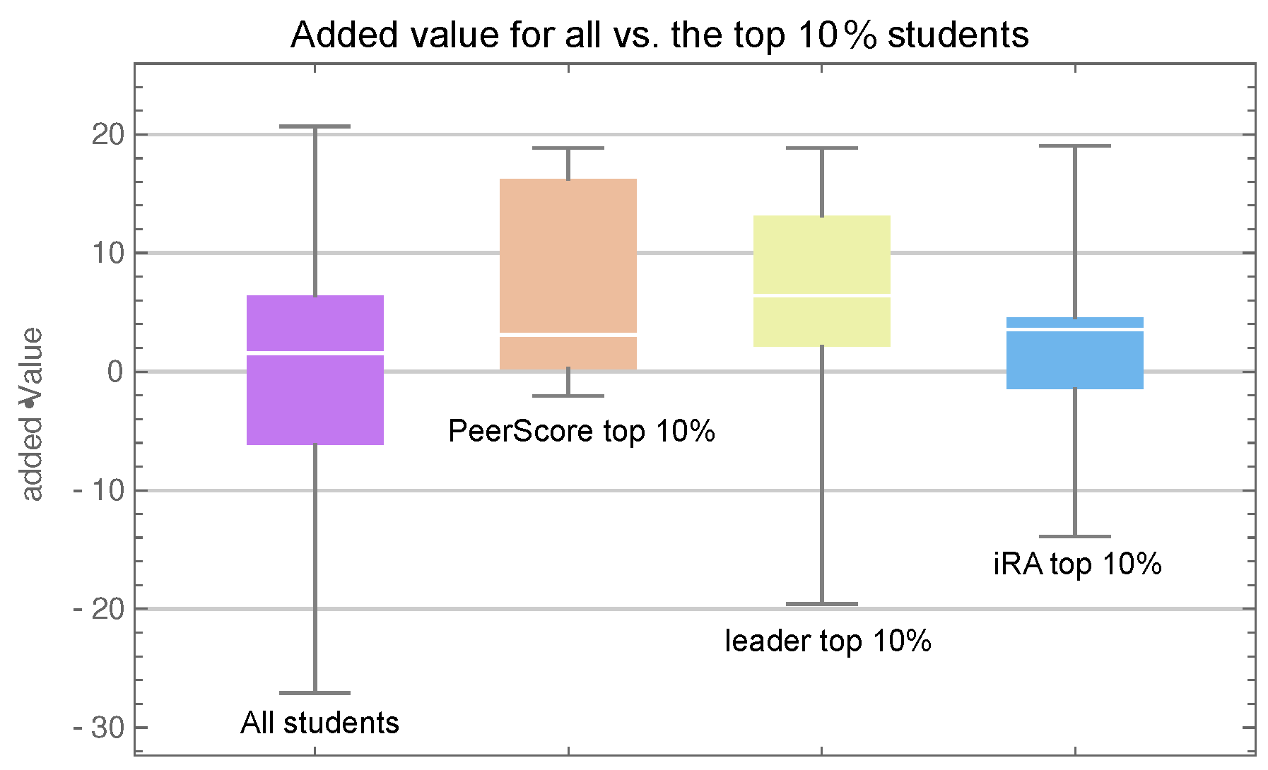
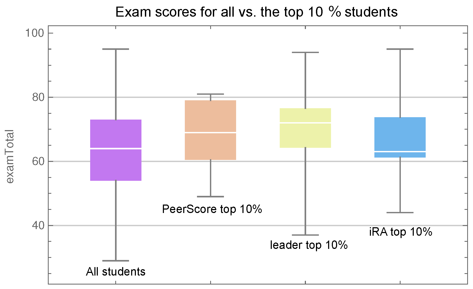
We identified three groups of students, each consisting of the top performers with respect to each variable (iRA, PeerScore, and leader), and we would naturally expect each of these groups to consist of talented and motivated students obtaining high exam scores. A graphical representation of the exam scores for these groups as well as the whole class is given in Figure 6, and we see that each group—with the possible exception of the sample with high iRA scores—did on average perform better than the average of the entire class. The plots indicate that the best performing group was the one with a high leader score and a Mann–Whitney–Wilcoxon u-test comparing that sample with the entire class yields a p-value of (the null hypothesis of the Mann–Whitney–Wilcoxon u-test is that a randomly selected value from one sample is as likely to be greater than as it is likely to be smaller than a randomly selected value from the other sample).
Besides this unconvincing p-value, the preceding analysis is unsatisfactory in the sense that it tells us very little about how much each identified group learned from the course. A large part of the course syllabus covers topics familiar to the students from their pre-university education, so initial knowledge is likely to be a confounder influencing all of the observed variables. We do however have an estimate of the students’ initial knowledge and their logical reasoning skill in the variables logic and , so we use these to build predictive models, following the method outlined in the previous section. Using logic and as predictors, we used DataModeler to construct a model ensemble whose median was used to predict each student’s exam score. Since the algorithm is probabilistic, the outcome may be different each time one runs it, but one model from the ensemble is given below:
Note that in (2), not all of the predictors were used. The power of genetic algorithms is that they automatically identify the relevant variables; i.e., we could load data from dozens or even hundreds of previous exams into DataModeler and it would identify only those few that are important to predict the calculus exam. For instance, notice that the pt1 score does not appear in (2), and hence is not important for this particular model. For (2), we have ; i.e., the first day logic and initial calculus knowledge tests explain about 63% of variation in the introductory calculus final exam score.
Recall that the Added Value defined by (1) is the residual of the model—i.e., the actual score (the final exam score in this quasi-experiment) minus the predicted score.
Now, using Added Values in place of raw exam scores, we repeat the previous exercise comparing the three identified groups. Figure 7 provides a graphical representation of the added values for these groups as well as the whole class. For example, we see that the median added value for the whole class (the horizontal line in the leftmost whisker plot) is very close to zero, which is to be expected. Indeed, the models are constructed in such a way that the average added value will be zero. Looking instead at the group with high iRA scores (the rightmost plot), we see that their added values—while having a positive median—are clustered near zero. That is, their exam scores agree with the predicted values, which means that their final exam performance was largely determined by the predictors (initial calculus knowledge and logic test result). For the other two groups, we can observe a positive outcome in added value. In other words, students who were rated highly by their team mates and students who were often selected as team leaders performed better at the final exam than we could predict from their initial level. Moreover, a Mann–Whitney–Wilcoxon u-test comparing the sample with high leader scores versus the entire class now yields a p-value of , which is better than the corresponding comparison with raw exam scores.
While our analysis still does not reveal whether being a team leader directly or indirectly causes you to perform above expectation at final exams, or whether the teams tend to select high performers and are better at doing so than our models could predict, it does at least suggest that a student’s involvement in the team activities of this TBL course was more indicative of course gain than high scores on individual readiness tests.
4. Results and Discussion
Our main contribution is an app [16] that allows the user to extract insights from data collected during the normal process of teaching a course. While it is not meant to replace a rigorous experimental setup, the current version which is built on a machine learning algorithm does provide a means of control for confounding factors, as long as these can be measured. To illustrate possible applications of the tool, two simple quasi-experiments have been described:
- In Quasi-experiment 1 we saw examples where clickers were a more effective instructional tool than handwritten homework, while online homework with immediate feedback and unlimited attempts seems to have been beneficial to students’ learning.
- In Quasi-experiment 2, we have seen that during an introductory calculus course taught with a TBL approach, high student involvement in team activities as measured by Peer Evaluations and Team Leader responsibilities was more indicative of course gain than high performance at individual readiness assessment quizzes.
In each example above, one might proceed to find explanations or conduct further, more elaborate, trials. The results of Quasi-experiment 1 can be interpreted in the sense that students do not view the grader’s handwritten comments on their handwritten assignments as feedback, which is consistent with literature on feedback (see [17]). Results of Quasi-experiment 2 can be interpreted in the sense that peer evaluation is a better tool for estimating the true motivation of a student than quizzes.
However, elaborating on our quasi-experiments is outside the scope of this paper, which is to illustrate how insight and ideas for further investigation can be extracted from data that are easily obtained from the normal process of teaching. While our process does not eliminate confounding factors not reflected in the predictors chosen for each quasi-experiment, we argue that with a sound choice of predictors the added value as defined in this paper will give a relevant measure of course gain.
Another observation we have made is that predicting written exams in university from previous written university exams has 70–80% accuracy. When we try to predict a university grade from pre-university grades, accuracy drops to about 60%, which is reasonable since university is quite a different environment from secondary school, junior college, or polytechnic. However, when we try to predict a project score from exam scores, accuracy is a mere 35%. In other words, by our observations, previous exam results are generally good predictors for future exam results but say very little about a student’s expected performance in project-based tasks. It would be very interesting to conduct similar quasi-experiments with oral exams, presentations, reports, and other methods of assessment.
5. Conclusions
We propose a methodology for educators to constantly improve their teaching by identifying teaching methods, instructional tools, and pedagogies that work best in their own classroom and acting upon findings. Of course, the decision to adopt one or another teaching method should be based on education research and on personal pedagogical expertise, but at the same time, it makes sense to extract meaning from data on students’ results that are generated as the courses are taught and augment the decision to make changes in the classroom with data-driven insights. Such a methodology can be called Data-Driven Classroom Tuning. It comprises the following four steps:
- (a)
- Flexible assessment: design the assessment structure that allows students to choose learning activities associated with teaching methods implemented in the course.
- (b)
- Initial level of preparation: acquire the students’ grades in previous courses, conduct a pre-test, collect background information (such as the degree programme)—everything that is available and that may be used to estimate confounding variables, such as diligence, talent, motivation, and pre-knowledge.
- (c)
- Predictive modelling: after the course ends and the final exam is graded, build a nonlinear mathematical model that predicts exam scores based on the initial level of students.
- (d)
- Residual: match the model’s residual (we call it Added Value here) to the preferred choice of learning activities.
To assist with our methodology in practice, an app that calculates added values and produces visuals was developed—see [16].
Our methodology is applicable under the assumptions that the course instructor is free to select teaching methods, instructional tools, and pedagogies (which is often not the case in secondary schools); that there exists the objective metric measuring students’ mastery of material when the course is over (which may not be the case in certain disciplines such as fine arts); and that data on students’ initial level are available (which is usually a matter of getting approval) and accurately predicts the metric of students’ success in the course (which can only be found by modelling after the course has ended).
The main novelty of our findings is in the methodology—machine learning-based analysis of non-experimental data on students’ scores. Besides, the fact that we compared the effectiveness of clickers and handwritten homework rather than evaluating the effectiveness of clickers alone is new. Finally, there exist very few if any studies on the effectiveness of clickers in teaching undergraduate mathematics. Our paper is one of the first studies on the effectiveness of clickers specifically in teaching undergraduate mathematics rather than psychology, nursing, combat life training, etc.
The main limitation of our methodology is that it is not a proper scientific method, at least not yet. We do not know whether the Mann–Whitney–Wilcoxon u-test is the right technique to evaluate the statistical uncertainty of the findings. We do not know what the “right” method of selecting groups who showed preference towards one or another learning activity should be. More quasi-experiments are required to establish reasonable limits for models’ precision within which our methodology is applicable.
Our methodology is for evaluating and comparing particular teaching methods rather than holistic pedagogies. In order to compare holistic pedagogies such as Peer Instruction [18] vs. SCALE-UP [5] vs. TBL [4], we need to create a situation when two courses with the same content, the same instructors, the same final assessment, and the same means of evaluation of students’ initial level of preparation are taught concurrently and yet differently. This seems to be quite a rare situation, although not entirely impossible.
The app that we have developed is free and is shared with the educational community. However, it runs on the proprietary software DataModeler, which in turn runs on another proprietary software—Wolfram Mathematica. In the future, we are planning to develop a free online version.
There are advantages of our methodology over traditional randomized experiments and quasi-experiments. Our methodology relies on non-experimental data collected by the university. The course instructor does not have to design the quasi-experiment in advance, and does not need a great deal of time, effort, and statistical knowledge to process data. Even if results of the quasi-experiment are undetermined, our app will still calculate Added Values. The instructor can just interview students who obtained a large positive or a large negative Added Value to look for the reasons of their success or failure.
Supplementary Materials
The following are available online at www.mdpi.com/2227-7102/8/1/7/s1: a PDF document with further data analysis of the first half of quasi-experiment 1.
Acknowledgments
This work is supported by EdeX grant “Does team-based learning improve exam scores”. The authors are also grateful to Irina Orlenko for her invaluable comments on the manuscript.
Author Contributions
Fedor Duzhin has created the concept of data-driven classroom tuning and designed quasi-experiment 1. Anders Gustafsson has designed quasi-experiment 2.
Conflicts of Interest
The authors declare no conflict of interest. The founding sponsors had no role in the design of the study; in the collection, analyses, or interpretation of data; in the writing of the manuscript, and in the decision to publish the results.
References
- Hattie, J. Visible Learning: A Synthesis of Over 800 Meta-Analyses Relating to Achievement; Routledge: Abingdon, UK, 2008. [Google Scholar]
- Becker, W.E. Quantitative research on teaching methods in tertiary education. In The Scholarship of Teaching and Learning in Higher Education: Contributions of Research Universities; Indiana University Press: Bloomington, IN, USA, 2004; pp. 265–310. [Google Scholar]
- MyMathLab; Pearson Education: London, UK, 2011.
- Michaelsen, L.K.; Sweet, M. The essential elements of team-based learning. New Dir. Teach. Learn. 2008, 2008, 7–27. [Google Scholar] [CrossRef]
- Beichner, R.J.; Saul, J.M.; Abbott, D.S.; Morse, J.J.; Deardorff, D.; Allain, R.J.; Bonham, S.W.; Dancy, M.H.; Risley, J.S. The student-centered activities for large enrollment undergraduate programs (SCALE-UP) project. Res. Based Reform Univ. Phys. 2007, 1, 2–39. [Google Scholar]
- Xu, J.; Han, Y.; Marcu, D.; van der Schaar, M. Progressive Prediction of Student Performance in College Programs. In Proceedings of the Thirty-First AAAI Conference on Artificial Intelligence, San Francisco, CA, USA, 4–10 February 2017. [Google Scholar]
- Kotsiantis, S.B. Use of machine learning techniques for educational proposes: A decision support system for forecasting students’ grades. Artif. Intell. Rev. 2012, 37, 331–344. [Google Scholar] [CrossRef]
- Chen, L.; Zitikis, R. Measuring and Comparing Student Performance: A New Technique for Assessing Directional Associations. Educ. Sci. 2017, 7, 77. [Google Scholar] [CrossRef]
- Vladislavleva, E.J.; Smits, G.F.; Den Hertog, D. Order of nonlinearity as a complexity measure for models generated by symbolic regression via pareto genetic programming. IEEE Trans. Evolut. Comput. 2009, 13, 333–349. [Google Scholar] [CrossRef]
- Freeman, S.; Eddy, S.L.; McDonough, M.; Smith, M.K.; Okoroafor, N.; Jordt, H.; Wenderoth, M.P. Active learning increases student performance in science, engineering, and mathematics. Proc. Natl. Acad. Sci. USA 2014, 111, 8410–8415. [Google Scholar] [CrossRef] [PubMed]
- Hake, R.R. Interactive-engagement versus traditional methods: A six-thousand-student survey of mechanics test data for introductory physics courses. Am. J. Phys. 1998, 66, 64–74. [Google Scholar] [CrossRef] [Green Version]
- James, G.; Witten, D.; Hastie, T.; Tibshirani, R. An Introduction to Statistical Learning; Springer: New York, NY, USA, 2013; Volume 112. [Google Scholar]
- DataModeler; Version 8.24; Evolved Analytics LLC: Midland, MI, USA, 2015.
- Oswald, H.; Allen, J.; Gough, B. Share LaTeX. Available online: https://www.sharelatex.com (accessed on 8 January 2018).
- Sisk, R.J. Team Based Learning: Systematic Research Review. J. Nurs. Educ. 2011, 50, 665–669. [Google Scholar] [CrossRef] [PubMed]
- Vladislavleva, K.; Stijven, S. Custom Notebook. Available online: http://tinyurl.com/edex-custom-notebook (accessed on 8 January 2018).
- Boud, D.; Molloy, E. Feedback in Higher and Professional Education: Understanding It and Doing It Well; Routledge: Abingdon, UK, 2013. [Google Scholar]
- Crouch, C.H.; Mazur, E. Peer instruction: Ten years of experience and results. Am. J. Phys. 2001, 69, 970–977. [Google Scholar] [CrossRef]
Figure 1.
Symbolic regression produces hundreds of models that can be visualized as a scatter plot on the plane complexity–error.
Figure 1.
Symbolic regression produces hundreds of models that can be visualized as a scatter plot on the plane complexity–error.
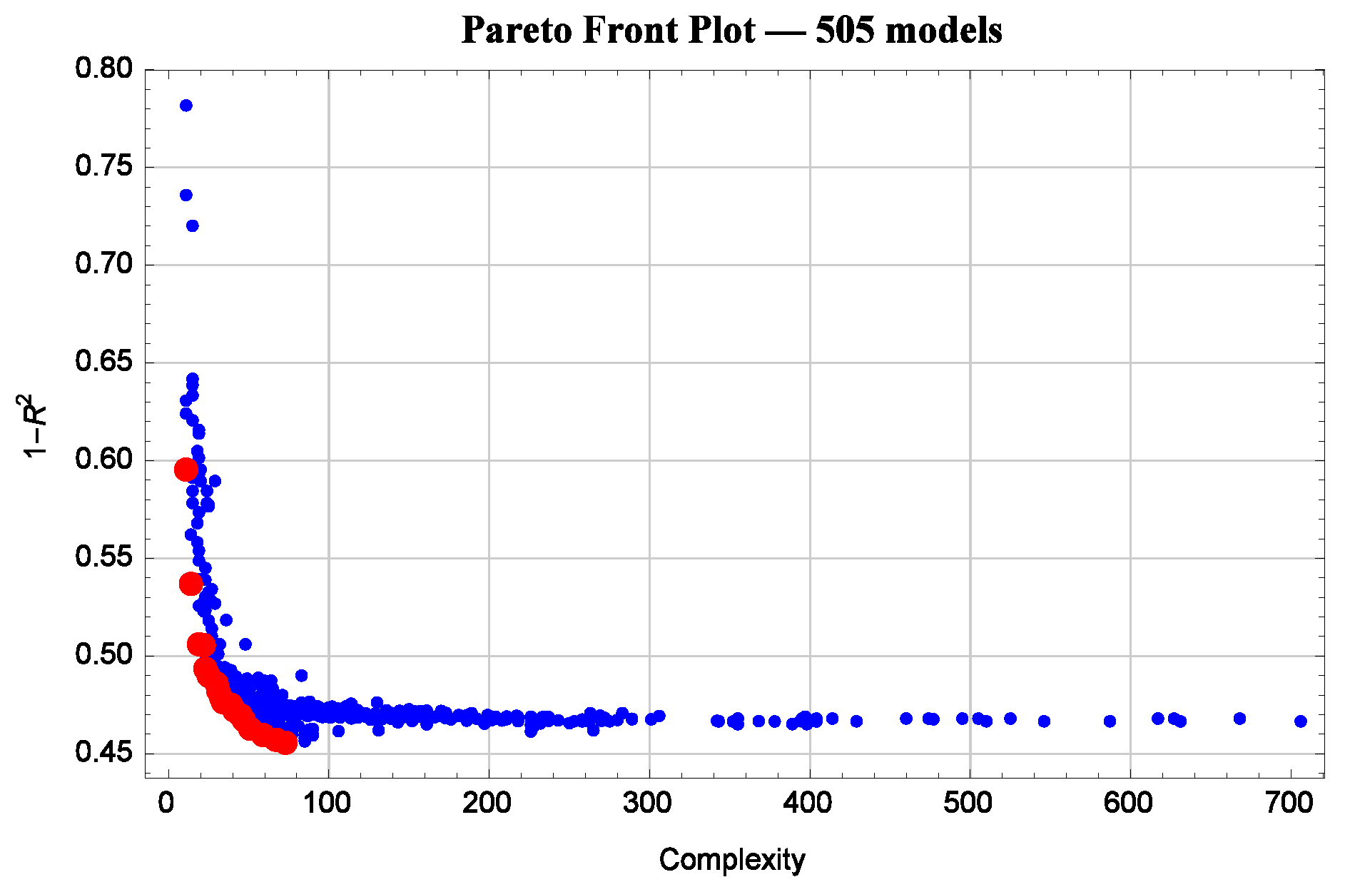
Figure 2.
Quasi-experiment 1. Left: scatter plot of written homework vs. clicker scores in 2015. Right: scatter plot of online homework vs. clicker scores in 2016.
Figure 2.
Quasi-experiment 1. Left: scatter plot of written homework vs. clicker scores in 2015. Right: scatter plot of online homework vs. clicker scores in 2016.

Figure 3.
Quasi-experiment 1: predictive models.
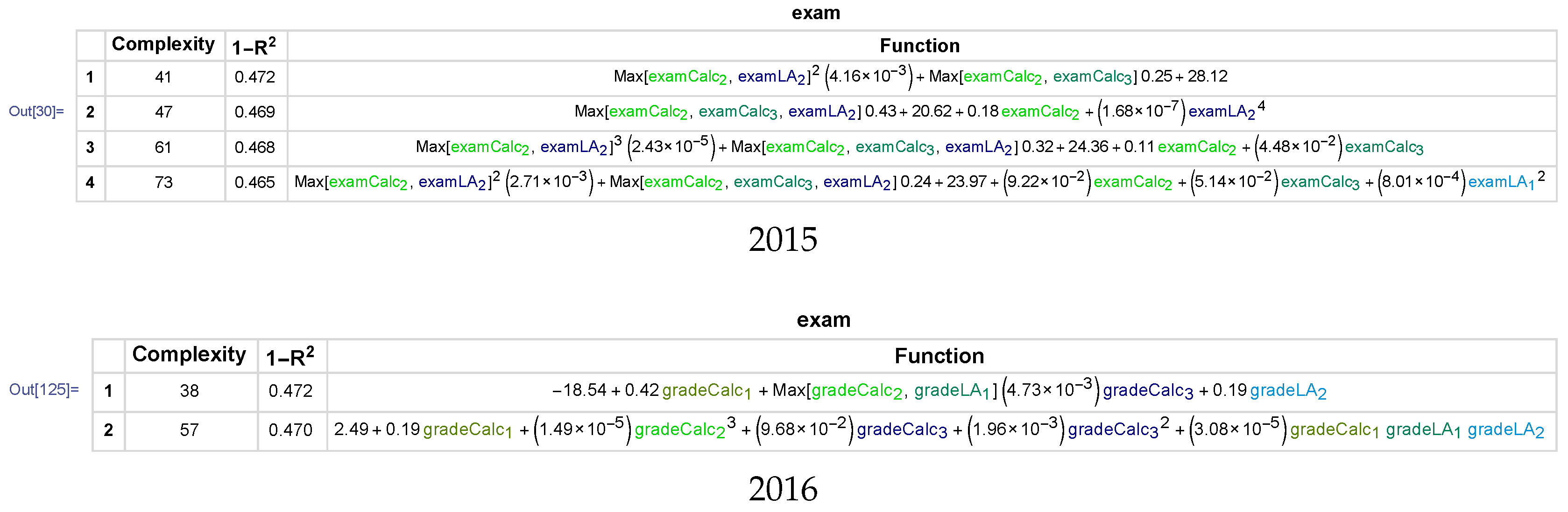
Figure 4.
Quasi-experiment 1. Left: raw exam scores of students who preferred clickers or handwritten homework in 2015. Right: raw exam scores of students who preferred clickers or online homework in 2016.
Figure 4.
Quasi-experiment 1. Left: raw exam scores of students who preferred clickers or handwritten homework in 2015. Right: raw exam scores of students who preferred clickers or online homework in 2016.

Figure 5.
Quasi-experiment 1. Left: added values of students who preferred clickers or handwritten homework in 2015. Right: added values of students who preferred clickers or online homework in 2016.
Figure 5.
Quasi-experiment 1. Left: added values of students who preferred clickers or handwritten homework in 2015. Right: added values of students who preferred clickers or online homework in 2016.
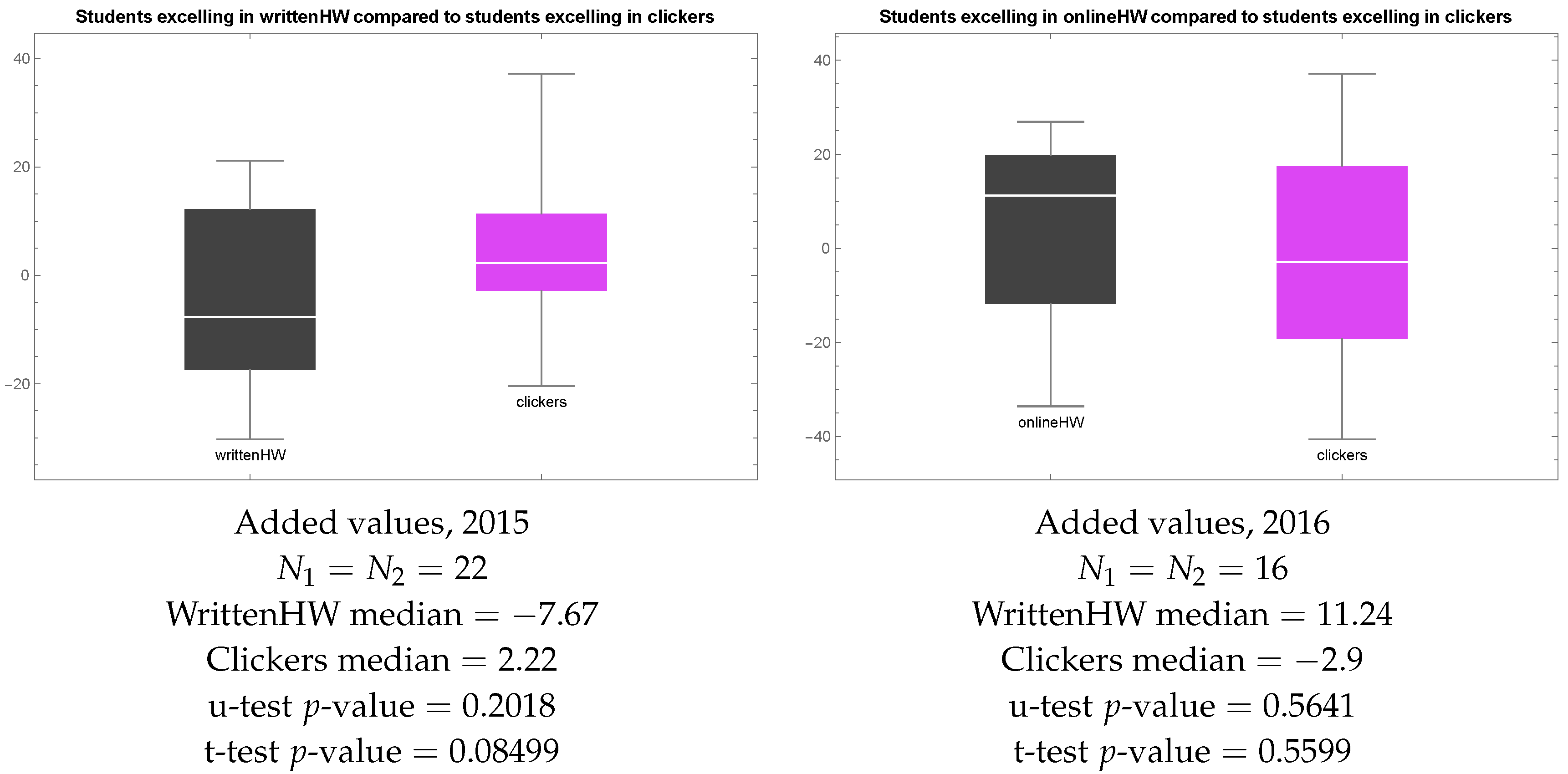
Figure 6.
Whisker chart showing (from left to right) final exam scores of all students, students with high PeerScore, students with high leader score, and students with high iRA score.
Figure 6.
Whisker chart showing (from left to right) final exam scores of all students, students with high PeerScore, students with high leader score, and students with high iRA score.

Figure 7.
Whisker chart showing (from left to right) added values of all students, students with high PeerScore, students with high leader score, and students with high iRA score.
Figure 7.
Whisker chart showing (from left to right) added values of all students, students with high PeerScore, students with high leader score, and students with high iRA score.

Table 1.
Hypothetical example. ACHEM: Analytical Chemistry; DTest: diagnostic test; ICHEM: Basic Inorganic Chemistry; PCHEM: Basic Physical Chemistry; Pred: predicted score.
Table 1.
Hypothetical example. ACHEM: Analytical Chemistry; DTest: diagnostic test; ICHEM: Basic Inorganic Chemistry; PCHEM: Basic Physical Chemistry; Pred: predicted score.
| Student | ICHEM | PCHEM | DTest | ACHEM | Pred |
|---|---|---|---|---|---|
| Alice | 98 | 95 | 92 | 89 | 88 |
| Brian | 60 | 94 | 72 | 85 | 74 |
| Cortney | 82 | 56 | 87 | 70 | 81 |
| Diane | 52 | 74 | 50 | 59 | 59 |
Table 2.
Summary of quasi-experiment 1: similarities and differences between clickers and homework (HW) in 2015 and 2016.
Table 2.
Summary of quasi-experiment 1: similarities and differences between clickers and homework (HW) in 2015 and 2016.
| 2015 | 2016 | |||
|---|---|---|---|---|
| N = 205 | N = 151 | |||
| Clickers | HW | Clickers | HW | |
| Mode | in class (2 h) | handwritten | in class (1 h) | online |
| Feedback time | immediate | 2 weeks | immediate | a few hours |
| No. of questions | 5 | 10 | 3 | 6 |
| Material coverage | 70% | 70% | 70% | 70% |
| Feedback type | aggregated | personal | aggregated | personal |
| Time | early morning | all week | early morning | all week |
| Familiarity | unfamiliar | familiar | unfamiliar | familiar |
| Collaboration | allowed | allowed | allowed | allowed |
Table 3.
Sample of 2015 data. Here, Calc1, Calc2, Calc3, LA1, and LA2 are exam scores in previous courses (predictors of the model), exam is the final exam score (response variable), and HW and clickers measure students’ effort into, respectively, handwritten homework and clickers.
Table 3.
Sample of 2015 data. Here, Calc1, Calc2, Calc3, LA1, and LA2 are exam scores in previous courses (predictors of the model), exam is the final exam score (response variable), and HW and clickers measure students’ effort into, respectively, handwritten homework and clickers.
| Student | Calc1 | Calc2 | Calc3 | LA1 | LA2 | HW | Clickers | Exam |
|---|---|---|---|---|---|---|---|---|
| Alester | 95.95 | 86.08 | 93.33 | 89.36 | 69 | 64 | 48 | 93.75 |
| Vaellyn | 79.73 | 73.42 | 47.78 | 60.64 | 79 | 26 | 41 | 77.5 |
| Hibald | 83.78 | 67.09 | 66.67 | 41.49 | 55 | 71 | 56 | 65 |
| Hotho | 89.19 | 83.54 | 75.56 | 71.28 | 84 | 51 | 81 | 80 |
| Leona | 81.08 | 35.44 | 41.11 | 65.96 | 55 | 47 | 0 | 36.25 |
| Oakenfist | 79.73 | 55.7 | 72.22 | 85.11 | 0 | 26 | 53 | 58.75 |
Table 4.
Sample of 2016 data. Here, Calc1, Calc2, Calc3, LA1, and LA2 are exam scores in previous courses (predictors of the model), exam is the final exam score (response variable); OnlineHW and clickers measure students’ effort into, respectively, online homework and clickers; project is the course project score.
| Student | Calc1 | Calc2 | LA1 | LA2 | Calc3 | OnlineHW | Clickers | Exam | Project |
|---|---|---|---|---|---|---|---|---|---|
| Amaya | 10 | 10 | 10 | 10 | 11 | 64 | 96 | 100 | 86.3 |
| Anara | 10 | 10 | 10 | 9 | 10 | 64 | 120 | 95 | 99.6 |
| Arthur | 11 | 10 | 10 | 10 | 9 | 60 | 84 | 95 | 87 |
| Arwaya | 8 | 8 | 8 | 7 | 8 | 35 | 108 | 60 | 99 |
| Shireen | 7 | 8 | 6 | 6 | 5 | 101 | 66 | 60 | 99.6 |
| Steffon | 9 | 9 | 7 | 8 | 8 | 60 | 90 | 65 | 111 |
| Samwell | 6 | 6 | 10 | 4 | 3 | 119 | 30 | 35 | 99.6 |
Table 5.
Sample of data collected during an introductory calculus class taught in 2016. Here, logic, , iRA, PeerScore, leader and exam are, respectively, the logic test score, the score from questions 1 to 11 of the initial calculus knowledge test, the average score from all Individual Readiness Assessments (iRAs), the score from the student peer evaluation, the number of times the student was a team leader, and the final exam score.
| Name | Logic | pt1 | pt2 | ... | pt11 | iRA | PeerScore | Leader | Exam |
|---|---|---|---|---|---|---|---|---|---|
| Student 1 | 0.5 | 1 | 1 | ... | 1 | 83.33 | 3.18 | 3 | 59 |
| Student 2 | 1 | 1 | 0 | ... | 1 | 72.5 | 0 | 6 | 53 |
| Student 3 | 0.5 | 1 | 0 | ... | 0 | 79.58 | 3.18 | 1 | 63 |
| Student 4 | 0.5 | 0 | 1 | ... | 0 | 56.25 | 5 | 77 | |
| Student 5 | 0.5 | 0 | 0 | ... | 0 | 74.58 | 3 | 68 | |
| Student 6 | 0.5 | 1 | 1 | ... | 1 | 77.5 | 0 | 5 | 71 |
| Student 7 | 0.5 | 1 | 0 | ... | 1 | 91.67 | 1 | 76 |
© 2018 by the authors. Licensee MDPI, Basel, Switzerland. This article is an open access article distributed under the terms and conditions of the Creative Commons Attribution (CC BY) license (http://creativecommons.org/licenses/by/4.0/).
Share and Cite
MDPI and ACS Style
Duzhin, F.; Gustafsson, A. Machine Learning-Based App for Self-Evaluation of Teacher-Specific Instructional Style and Tools. Educ. Sci. 2018, 8, 7. https://doi.org/10.3390/educsci8010007
AMA Style
Duzhin F, Gustafsson A. Machine Learning-Based App for Self-Evaluation of Teacher-Specific Instructional Style and Tools. Education Sciences. 2018; 8(1):7. https://doi.org/10.3390/educsci8010007
Chicago/Turabian StyleDuzhin, Fedor, and Anders Gustafsson. 2018. "Machine Learning-Based App for Self-Evaluation of Teacher-Specific Instructional Style and Tools" Education Sciences 8, no. 1: 7. https://doi.org/10.3390/educsci8010007
Note that from the first issue of 2016, this journal uses article numbers instead of page numbers. See further details here.