
Bayesian Framework for Multi-Wave COVID-19 Epidemic Analysis Using Empirical Vaccination Data


1
Department of Statistics, East China Normal University, Shanghai 200062, China
2
KLATASDS-MOE, School of Statistics, East China Normal University, Shanghai 200062, China
3
Department of Statistics, University of Haifa, Haifa 3498838, Israel
4
ECNU-UH Joint Translational Science and Technology Research Institute, Shanghai 200241, China
*
Author to whom correspondence should be addressed.
Mathematics 2022, 10(1), 21; https://doi.org/10.3390/math10010021
Submission received: 10 November 2021
/
Revised: 15 December 2021
/
Accepted: 17 December 2021
/
Published: 21 December 2021
(This article belongs to the Special Issue Machine Learning and Statistical Modeling with Applications in Real-World Data and Artificial Intelligence)
Abstract
:The COVID-19 pandemic has highlighted the necessity of advanced modeling inference using the limited data of daily cases. Tracking a long-term epidemic trajectory requires explanatory modeling with more complexities than the one with short-time forecasts, especially for the highly vaccinated scenario in the latest phase. With this work, we propose a novel modeling framework that combines an epidemiological model with Bayesian inference to perform an explanatory analysis on the spreading of COVID-19 in Israel. The Bayesian inference is implemented on a modified SEIR compartmental model supplemented by real-time vaccination data and piecewise transmission and infectious rates determined by change points. We illustrate the fitted multi-wave trajectory in Israel with the checkpoints of major changes in publicly announced interventions or critical social events. The result of our modeling framework partly reflects the impact of different stages of mitigation strategies as well as the vaccination effectiveness, and provides forecasts of near future scenarios.
1. Introduction
Throughout a typical outbreak of COVID-19 in a certain country, the first stage of the pandemic is most likely to have a trajectory with exponential growth [1], which is plausibly explained by commonly used statistical models, e.g., the epidemic growth models, such as the Gompertz model [2], or compartmental models [3,4].
However, due to the fact that the COVID-19 pandemic has been hitting most countries worldwide with various patterns of epidemic development for over one year, multiple waves of infection growth have emerged after the initial phase; see [5]. Observing a complete epidemic trajectory of COVID-19 in a certain country, what we could commonly expect is an initial wave of exponential growth followed by multiple waves seperated by corresponding change points. The change points indicate the nationwide changes of effective factors, including mitigation measures [6], containment policies, groups of imported cases, social movement and large-scale clustering events, increasingly infectious variants for pandemics, etc. Considering the complexities, a typical deterministic model with a fixed set of parameters could hardly handle the explanatory analysis of the complete epidemic trajectory due to the limitation of real data and the shifting dynamics corresponding to change points. Hence, the integrated modeling class, such as piecewise models, will unfold the functionalities adapted to trajectories featuring long-term study periods.
Vaccination is another essential factor that considerably affects the transmission of COVID-19, especially for the recent circumstances in numerous countries which have accomplished millions of injections of vaccine doses; see [7]. Unlike most of the other pandemics in the past, thanks to the open source of empirical vaccination data, the exact numbers of daily vaccinations can be directly implemented in the model instead of being approximated through the complex dynamics. Though the vaccination has not produced any impact until the inoculations facilitated by the government, which normally began at the latest phase of the epidemic [8], it enables a substantial decline on susceptible individuals; see [9,10]. Thanks to the high protection rate [11] and the continuously increasing population of vaccinated individuals, the vaccination has brought an obvious influence on the long-term study of the epidemic trajectory.
The ODE-based compartmental models, such as the susceptible–infected–recovered (SIR) model [12,13], play a dominant role in the studies of epidemic outbreaks for infectious diseases. This typical class of methodologies, which simulates population compartments and their shifting ratios from one to another (e.g., the susceptible individuals become infectious), mainly focuses on the estimation and prediction of the epidemic trajectories and effectiveness of containment measures. Based on the idea of depicting the multi-wave trajectory of a country with a highly vaccinated population, in our study, we establish a parsimonious dynamic system of the susceptible–exposed–infected–recovered (SEIR) model [14,15,16] which is modified by piecewise modeling and the additional usage of empirical vaccination data. Parameter inference that competently reflects the corresponding trajectories remains a critical issue for the model calibration. Among them, the transmission rate is particularly sensitive to epidemic changes emerged at different checkpoints throughout the full study period. Hence, the Bayesian framework [17] is utilized for the inference of parameters, due to the complexities and insufficient data of modeling.
Various Bayesian methods have been employed for the epidemiological and related models for studying COVID-19, including the Bayesian MCMC algorithm for the inference of statistical and epidemiological parameters [18,19,20,21], Naïve Bayes method for feature classification in the diagnosis of COVID-19 [22], Bayesian network for severity classification [23,24], spatial geo-referencing analysis [25,26], etc. A few studies have already presented remarkable attempts on methodologies that integrate Bayesian inference with SIR-based compartmental models. Hao et al. [27] proposed an extension of the standard SEIR model, which specifically accounts for asymptomatic and pre-symptomatic individuals. This model, featuring population movement and time varying ascertainment rates, was applied to the initial wave of COVID-19 epidemic in Wuhan, where the confinement measures could be explicitly identified. Bhaduri et al. [28] proposed another modification of the SEIR model, which considers not only asymptomatic infectives, but containment measures and the potential effect of misclassifications (false negative rate) in consequence of testing error. The study demonstrated the effectiveness of the model which was applied to the outbreak in India up to the summer of 2020. As a typical Bayesian approach, the Markov Chain Monte Carlo algorithm was applied for adequate parameter inference in both studies.
With the similar objective for the explanatory analysis of a multi-wave COVID-19 epidemic with change points, some of the related studies are briefly summarized below. Bherwani et al. [29] presented a change point analysis (CPA) that utilizes the Bayesian probability model (BPM) to understand the changing aspects of COVID-19 penetration within the states of India, suggesting that the states which implemented the lockdown before the exponential rise of cases have been able to control the spread of the disease in a very efficient way. Dehning et al. [5] developed a Bayesian framework based on MCMC sampling to the fundamental SIR model for the spread of COVID-19 to characterize central epidemiological parameters, the temporal change of the spreading rate and the potential change points, and the timing and magnitude of intervention effects. Mbuvha and Marwala [30] further applied this approach on a SEIR model, which succeeded in depicting the short-term multi-wave trajectory of South Africa. Other mathematical methodologies have been developed to solve the multi-wave issue as well. Salvadore et al. [31] presented an integro-differential approach to model the wave-like COVID-19 dynamics that accounts for typical evolution parameters. The model started with a Lotka–Volterra equation, and further included a temporal dependency for the transmissibility consisting of the evolving environmental conditions, where vaccinations, virus variants, and various containment strategies were included. The optimal parameters were calculated for each Italian region separately. Beira and Sebastião [32] conceived a comprehensive PSEIRD(S) model to fit the data sets related to the infected, deceased and hospitalized cases reported for the severe post-Christmas outbreak in Portugal. Some of the model parameters fitted vary discretely with time, which indicates different scenarios of various epidemic waves. Cacciapaglia et al. [33] proposed a consistent picture of the wave pattern based on the epidemic renormalization group (eRG) framework. The results demonstrated that the key to control the arrival of the next wave of the pandemic is the strolling period between waves. As a direct extension of [33], Cot et al. [34] employed the eRG framework supplemented with the implementation of vaccination to reproduce and predict the COVID-19 pandemic across the U.S. The study suggested that vaccinations alone are not enough to curb the current and the next waves, and strict social distancing measures should keep being enacted until herd immunity is achieved.
In our study, we aim to solve the issues of explanatory analysis on the long-lasting multi-wave epidemic with the ongoing large-scale vaccination campaign; thus, we integrate Bayesian inference with an extended compartmental SEIR model featuring the new factor of vaccination and the time-varying transmissibility [35] that aligns with multiple waves in the full epidemic trajectory. To interpret the time dependence, we exert specific change points which are potentially driven by assorted causes like governmental containment measures, nonpharmaceutical interventions [36], clustering events, mutation influence or vaccination impact [7]. We propose a Bayesian framework that is mainly designed for the long-term study of the epidemic trajectory featuring multi-waves with several change points. Aiming to yield an explanatory analysis for the dynamic epidemic growth, especially including the recent scenarios with vaccinations, we accomplish a complete process of Bayesian inference of the time-varying transmissibility along with respective uncertainties of epidemiological and statistical parameters based on the real data in Israel. We believe that our modeling framework is simple and applicable to other countries and regions that are suffering from long-term situations of the COVID-19 pandemic.
The structure of this article is organized as follows. Section 2 offers a manifest description of the real data for modeling. Section 3 elaborates the detailed methodologies for our modeling framework. Section 4 demonstrates the complete results for model inference. Conclusions and discussions are given in Section 5.
2. Materials
2.1. Source of Data
The state of Israel is selected as the studied country for our model deployment. We employ the exact number of COVID-19 confirmed positive cases in Israel using the data from 21 February 2020 (the date of the earliest case reported) to 28 September 2021 via the official websites of World Health Organization. The vaccination data are retrieved via Israel Ministry of Health and the dashboard of ’Our World in Data’. All cases are laboratory confirmed.
2.2. Data Description
As the first country in the world to double-vaccinate the majority (over 50%) of its population, Israel is one of the leaders in fighting against the spreading of the pandemic thanks to its prompt roll-out of COVID-19 vaccines [37]. However, the number of newly reported cases still keeps spiraling in the fourth wave of the epidemic, though Israel has tried almost every effort of intervention, including severe extent of social distancing, banning gathering, workplace and school closures, travel controls, contract tracing, and restrictions on internal movement.
The first case of COVID-19 in Israel was officially confirmed on 21 February 2020 when a female citizen tested positive after returning from her quarantine on the highly infected Diamond Princess ship in Japan [38]. The infection remained at a steady pace under mild interventions until a sudden surge occurred in the third week of March. On 19 March, a national state of emergency was officially declared, which brought about legal enforcement of lockdown restrictions [39]: ’staying home unless absolutely essential.’ The lockdown revealed effectiveness when the number of newly infected cases substantially fell into single digits in May, and thus, the government gave the approval of reopening the economy with restrictions gradually being eased [40].
However, the epidemic staged a comeback with the daily number climbing up to 100 again at the end of May, indicating a more influential and persistent second wave of the pandemic. Numerous regional or nationwide lockdowns were carried out aperiodically with restrictions of both governmental interventions and non-pharmaceutical interventions in consideration of the continuous tradeoff between containment and economic reopening, which unexpectedly led to a rapid escalation starting from August. On 10 September 2020, Israel became the country with the highest rate of COVID-19 infections per capita [41]. A new record of over 9000 daily cases was reached at the end of September, and the second wave of epidemic remained unpromising, owing to various reasons, including the summer vacation and several national holidays, large-scale religious events, protests voicing frustration over the response of the local government to the pandemic [42], and the worldwide epidemic explosion (especially in the U.S. and Europe, which are closely connected to Israel by international travel for the recall of Israelis abroad). Confidence decayed as people became impatient with immoderate restrictions and less alert to the spreading of COVID-19 because of its comparatively low severity rate; therefore, the daily cases scarcely declined.
Right after that, a more serious third wave took place from mid-November 2020. On 24 December 2020, the government declared a third nationwide lockdown (that began on 27 December) with more rigorous restrictions, including indoor gatherings of fewer than 10 people personal traveling limited within a 1000-meter radius from home, etc.; see [43]. Aiming to guard against the potential burst from celebrations of Christmas and New Year’s Eve, the lockdown was strictly implemented for 12 days until a set of tightened restrictions was renewed with updates, such as indoor gatherings of 5 people and the complete closure of Ben Gurion International Airport. The tightest lockdown, which consists of short-term curfews at times, was eventually extended to 7 February 2021. However, the interventions hardly effected a radical cure on the resurging of the epidemic, with a new daily record of over 10,000 reported cases. Though costly in economy, the third lockdown was the checkpoint for the majority of Israelis to become vaccinated against COVID-19. After the first dose of Pfizer vaccine administered on 19 December 2020 [8], a tremendous escalation of vaccinations appeared with the support of Green Pass policies implemented by the Israeli government on 21 February 2021, which granted exclusive permission for entry into hotel, theaters, gyms, and religious places, such as synagogues, etc.; see [44]. In order to return to normal life, most Israel residents restored their motivation on being fully vaccinated (i.e., two doses); hence, substantial drops were observed starting from the end of March. From April to June 2021, the period after the nationwide vaccination campaign, there unfolded a stable situation, which manifestly benefited from the high vaccinated rate of the population.
Technically, Israel almost reached herd immunity in June when the daily new cases were down to 0 for some days and people’s lives became almost normal; however, in the last phase of June 2021, daily case numbers began rising again. Mainly caused by the prevalent SARS-CoV-2 B.1.617.2 Delta variant with a much higher epidemiological spreading rate [45], Israel stepped into the fourth wave inevitably [46], and mild interventions with basic restrictions, such as requirement of mask-wearing and travel limitation, were reinstated to slow down the raging transmission of the Delta variant. Up to October 2021, with thousands of daily infected individuals, the ’fourth wave’ has not yet come to an end and the circumstance of future epidemic in Israel remains unclear. Figure 1 briefly demonstrates the multi-wave trajectory of daily new cases in Israel. Even though Israel is the pioneering country on the third vaccination for the booster shot, which practically started in July 2021, the statistics of reinfected individuals and the protection effectiveness remain to be validated. Therefore, in our study, we only focus on the vaccination data for the first doses (over 6 million) and the second doses (over 5.5 million), while excluding the third doses since we temporarily do not consider the complex situation with reinfected individuals.
3. Methods
To technically present the Bayesian framework designed for our epidemic analysis, two statistical modeling parts are elaborated, respectively, in the following context.
3.1. Epidemiological Model
For the analysis of the COVID-19 epidemic, compartmental models are widely used to quantify the transmissibility of disease, as well as depicting the dynamics between infected and uninfected populations. In our study, we apply the susceptible–exposed–infected–recovered (SEIR) compartmental model that has been dominant in the COVID-19 modeling literature. The SEIR model depicts the transition of individuals between 4 stages of conditions, namely, S —susceptible, E—exposed, I—infected, and R—recovered. Note that the difference between compartments of E and I mainly relies on whether the infection of an individual is confirmed. If not, we consider it an exposed individual who remains in incubation and will probably become infectious, while an infected individual should be removed from the compartment of the susceptibles. For the study of COVID-19, the additional compartment of ’E’ is necessary, considering the non-negligible incubation period under high transmissibility of the disease. Hence, we select the SEIR model, rather than the simpler three-compartment susceptible–infectious–recovered (SIR) model, to be the fundamental epidemiological model in our Bayesian framework.
From the perspective of statistics, the SEIR model can be interpreted as a four-state Markov chain model [30]. The dynamic behavior of the SEIR model relies on solving the following system of ordinary differential equations which depict the analytic trajectory of the infectious disease:
where and R represent the populations of the susceptible, exposed, infected and recovered, respectively. N is the total population, i.e., . and correspond to the transmission rate and the recovery rate, while is set to be the rate for individuals in incubation becoming infectious. Thus, and stand for the incubation period [47] and infectious period; see [30]. The basic reproductive number () is defined by .
Aiming to analyze the multiple waves in the epidemic trajectory of COVID-19, we consider the modeling design by Dehning et al. [5] as a piecewise SEIR model segmented by change points. Different sets of epidemiological parameters are applied for corresponding periods, that is, for the th period. However, since no breakthrough has been yielded in the clinical treatment of COVID-19, we simply retain the value of throughout the whole study period.
In order to fit the current development of COVID-19 pandemic, we specially extend the typical SEIR models with new variables of vaccinations. Considering the fact that most types of the COVID-19 vaccine employed worldwide (including Pfizer-BioNTech, Moderna, Astrazeneca, Johnson & Johnson, etc.) require two doses of injection, we add two variables, and , to measure the numbers of daily new cases that have completed the first and the second doses of injection, respectively, and and as the corresponding rates of vaccine efficacy. Note that this extended version of SEIR model differs from the typical compartmental models with vaccination, e.g., SIR-V [9,10,48], since we intend to apply the exact numbers of daily vaccination. Thanks to the open source of precise data on daily vaccinated cases, there is no need to treat V as an additional compartment with unknown values which require to be approximated via the complete dynamic system. Our extended version of SEIR model is summarized as follows:
where . Correspondingly, the change points are defined as , forming periods as represent the first day and the ending day of our complete study. The full time series of one compartment is an ordered joint set of values in periods, e.g., . In our study, we solve Equation (2) with a discrete time step day and for the real data of Israel.
3.2. Model for the Reported Cases
Similar to the definition from a basic SEIR model, the value for the number of daily incidences is proportional to the number of people leaving the E compartment, i.e., ; see [14]. Additionally, we set a new parameter for the ratio of reported cases, i.e., . Following the former work of [5], several auxiliary parameters, including the reporting delay D, the amplitude and phase for weekly modulation, are also considered in the modeling process to precisely depict the non-negligible delay and systematic variation of case reporting (i.e., lower numbers at weekends and accumulating reports during the weekdays). Note that the reporting delay is essential since there always exist circumstances where the individuals take rapid tests by themselves without uploading the positive results in time. Hence, the final expression for simulated daily reported cases from our model could be written as follows:
where implies the number of incidences for the corresponding day, and where as the reporting fraction. See Figure 2 for a sample plot of , where a 7-day cyclic period is demonstrated manifestly.
3.3. Bayesian Framework
Mainly following the statistical framework of [5], we construct a typical process of Bayesian inference for the estimation of parameters in our extended SEIR models. The Bayesian framework practically realizes the posterior inference of parameters by updating prior beliefs through customized likelihood [17]. Theoretically, the Bayesian inference is generally based on the Bayes theorem [49] as follows:
where is the posterior of the parameter vector , given the model M. stands for the observed data, which will be denoted as (for the reported cases of day T) in the following context, while is the likelihood and the evidence. In our study, consists of 24 parameters,
In Bayesian inference, the likelihood is a critical step that partially determines the effectiveness of the modeling. Here, in our Bayesian framework, the likelihood manifests the probability of observing the real data of reported cases. Suggested by Dehning et al. [5], a Student’s T distribution affiliated to the daily new cases is used to construct the likelihood function:
where is the location parameter, is the scale parameter, and is the degree of freedom. Note that the parameter , which is also in the parameter space , is a scaling factor tuning the spread of the distribution. The Bayesian inference based on the MCMC algorithm provides parameter estimation that lessens the discrepancy between the fitted number (for any time point T) and the corresponding real data ; thus, it statistically quantifies the similarity between the predicted cases derived from the model (3) and the real-world time series for observed reported cases. The distribution around the mean is similar to a Gaussian one; however, with heavy tails, it enhances the robustness of MCMC with respect to outliers, i.e., reporting noise [50]. The spread (i.e., the scale parameter ), motivated by observation noise through subsampling [51], is highly dependent on the number of daily cases. This design forms a variance proportional to the mean of the Student’s T distribution. Note that the general assumption of neglecting noises in the dynamic process is used since the SEIR compartmental model is fully deterministic.
3.4. Prior Specification
The empirical prior knowledge is taken into consideration in a Bayesian setting while obtaining reasonable parameter estimation for epidemic analysis and short-term forecasting. The elicitation of prior knowledge for the epidemiological parameters (e.g., ), the transmissibility and recovery rate of the disease, the mechanisms of the spreading trajectory, etc., is based on former studies (or expertise knowledge) with preliminary estimation from other countries and regions or from another closely related pandemic contagion. Based on expertise and empirical knowledge, the setting of prior distributions of plays an important role for parameter estimation. On the other hand, for the epidemiological parameters in our model, such as spreading rate , recovery rate , infectious rate , change points based on epidemiological periods, etc., their priors are specified with expectation values that are referred from related studies.
The detailed prior distributions of all the parameters are fully listed in Table 1. Mainly following the former study by [5], we select log-normal distributions for the transmission rate and recovery rate such that the initial basic reproduction number [20,52] equals a median of . The infectious rate is set to have the log-normal prior, which is equivalent to the mean incubation period of 5 days. Additionally, we also choose a log-normal prior for the reporting delay to incorporate both the mean value of the incubation period with median 5 days plus an assumed 3 days delay from being infected to being reported; see [53].
We recognize the change points in consideration of the Stringency Index proposed by the research project of ’Oxford COVID-19 Government Response Tracker’ along with checkpoints for the change in governmental intervention policies and nationwide events; see Figure 3. The Stringency Index is a composite measure based on 9 response indicators, including school closures, workplace closures, and travel bans, rescaled to a score value from 0 to 100, which is proportional to the strictness of governmental interventions; see [54].
As a result, we roughly treat 7 May 2020 as the first change point when the exit strategy was implemented after the first wave of epidemic boost; see [40]. From Figure 1, we notice the obvious two-stage pattern of escalation within the duration of the second wave, manifesting that an additional change point should not to be ignored. Indicated by the following trough in the curve of the Stringency Index, 17 August 2020 is picked as the second change point. In the same manner, by recognizing the substantial bottom of a certain period in the trajectory of the Stringency Index, we set 31 October 2020 as the starting point of the durable third wave and 15 June 2021 as the beginning of the current wave (the ’fourth wave’) as well as the division between the pre-Delta and post-Delta periods. Normal distributions with a standard deviation of 3 days are applied to construct the priors for , , and . Note that we keep the same prior for , , , and (also similar to ) since we are uninformed of the exact transmission rates after the initial phase of the pandemic, which will lead to a greater weight on the data-driven likelihood [30].
The parameters of initial infected individuals , initial exposed individuals and the scale factor for the likelihood are constrained by non-informative priors. The half-Cauchy distributions are employed with corresponding expectations.
Similar to the modeling design in [5], we construct a non-negative sine function (applying absolute values) with a total period of 7 days to modulate the number of daily cases; hence, we select a weakly informative prior (equivalent to the mean of 0.7 and the standard deviation of 0.17) for the amplitude of weekly modulation , along with a prior as a nearly flat circular distribution for the phase .
We give the proportion of reported cases a weakly-informative prior, which indicates that we are quite uncertain about this parameter, except that it stays within the interval of but should not be close to 1. For the remaining two parameters, and , which respectively stand for the efficacy of the first and the second dose of COVID-19 vaccine, we propose normal distributions with corresponding mean values for these priors. According to Pfizer data published in December 2020 [11], the Pfizer-BioNTech vaccine is roughly 52% effective after the first dose with 95% protection rate for fully vaccinated people. Though the Pfizer-BioNTech vaccine is not the only one distributed in Israel (Moderna and Pfizer-BioNTech are the two manufacturers available to the population of Israel), we still adopt these authenticated data since the two vaccines were similarly developed based on the same mRNA sequence, resulting in little difference on clinical efficacy. Table 1 summarizes the prior distributions of all the parameters described above.
3.5. Markov Chain Monte Carlo (Mcmc) with No-U-Turn Sampler (NUTS)
We adopt the MCMC algorithm as a straightforward and plausible approach for the effective inference of the posterior distributions on the parameters constructed; see [55,56]. MCMC works by drawing a sequence of dependent samples from the posterior distribution under circumstances, where it is unlikely for a direct draw of independent samples. With the algorithm, a Markov chain is created (representing a draw at the state of fictitious time t) such that
The main advantage of the MCMC approach for our complete model is that the full covariance matrix of is used; see [57]. Posterior inference on is carried out by random samples from the conditional distribution given the observation data, i.e., the reported cases of day T, and it follows from Equation (4) that
As one of the most frequently used methods in practice, the Metropolis–Hastings (MH) algorithm [58,59] is a simple and well-known MCMC method for generating a Markov Chain which converges to the target distribution. The MH generates a candidate from a proposal distribution with acceptance ratio
In most cases, a symmetric random walk is applied as the common proposal distribution, which is obtained by adding a Gaussian noise to a former state of the parameter. However, the proposal distribution with the random walk behavior often brings about a relatively low sample acceptance and limited sizes of effective samples. To overcome the shortage, the Hamiltonian Monte Carlo algorithm (HMC) was proposed by [60] to reduce random walk behavior by adding an auxiliary momentum variable to each parameter space . The basic idea of HMC is to employ the current gradient to assign a direction heading for the next state with a high probability. In general form, the HMC dynamic system, consisting of model parameters and the auxiliary momentum variables r, is denoted by the Hamiltonian , written as follows:
where signifies the negative log-likelihood of the posterior. From the perspective of the Hamiltonian, this equation could be referred to as a combination of the potential energy and kinetic energy , which is specified by a Gaussian kernel with the covariance matrix [61].
and the Hamiltonian dynamics for Equation (10) (at a fictitious time t) is defined as follows:
During the standard procedure of HMC, the leapfrog integrator discretizes the dynamical trajectory of Equation (10). Within the leapfrog integrator, a doubling process, which includes a half step in the direction of r, followed by a full step (with a discretization stepsize ) in the direction of , then ending with another half step in the same direction as the first half step, is operated to reach the next point of the path. Following the process of the Metropolis–Hastings algorithm, the newly derived parameters take the probability of acceptance as follows [62]:
The effective performance of HMC strongly relies on selecting adequate values for the discretization stepsize and the trajectory length L. Reasonable tuning for these two parameters is crucial for efficient sampling. Therefore, the No-U-Turn Sampler (NUTS) is applied as an extension of HMC that eliminates the need for specifying a value of L as well as retaining the capacity to inhibit random walk behavior; see [30,63]. In short, NUTS automates the tuning of and L. Specifically, is tuned via an initial burn-in phase by assigning a target mean acceptance probability, while L is chosen by adding extra steps iteratively until the trajectory starts to retrace itself, or descriptively speaking, to make a ’U-turn’.
NUTS suggests a recursive algorithm, which is a revised version of the doubling procedure based on slice sampling [64], thus a slice variable u is introduced with a conditional uniform distribution:
where the normalization constant , with as the logarithm of the density of . This procedure aims to sample above the slice of the posterior within a targeted bandwidth so as to guarantee the acceptance. After resampling, the Leapfrog integrator is implemented with steps taken back and forth to portray the path, which includes the first 1 step, then 2 steps, and 4 steps afterwards, etc. Hence, a balanced binary tree is constructed with leaf nodes corresponding to the position-momentum states. The signal for a stop is when the trajectory from the leftmost to the rightmost nodes of any subtree begins to double back (i.e., make a ’U-turn’). NUTS keeps doubling the tree at a height j until the condition is achieved that all the balanced binary subtrees have positive values of height, and the doubling process is halted when one of these subtrees with states associated with the leftmost and rightmost leaves and satisfies the following condition:
An upper boundary (usually, we take a large positive number, such as 1000) is set to be the second rule: we simply stop doubling if the tree includes a leaf node whose state satisfies
To summarize, Algorithm 1 elaborates the complete process of our Bayesian modeling framework. Note that for simplicity, Algorithm 1 is written in a pseudocode in Visual Basic.
| Algorithm 1 Complete modeling framework |
|
4. Results
We propose a novel Bayesian framework combining a modified piecewise SEIR model with an empirical model on daily reported and vaccinated cases in Israel, which captures both the change points in the long-term multi-wave trajectory and oscillations in the short-term period. Reporting delay and reporting fraction are considered to justify the fitness of the model.
To approximate the posterior distributions, four independent Markov Chains are performed with 1000 burn-in (tuning) steps and 5000 samples for each chain of the sampler. In our study, we apply the model and algorithm to the real data from 21 February 2020 to 28 August 2021 (as the ending day ), while leaving 30 days (from 29 August 2021 to 27 September 2021) for prediction. According to the population of Israel in 2020, we use an approximate number of 9.2 million as the known value for N.
The detailed posterior results of our extended SEIR model using NUTS are presented as follows. Figure 4 portrays the prior and posterior distributions of our modified SEIR model parameters. Figure 5 demonstrates the comparison between the real multi-wave trajectory and the results of daily incidence obtained directly from our modified SEIR model, where a smooth curve (free from noise) is fitted without the calibration of the reporting delay and the weekly modulation (which definitely adds noise to the yielded SEIR results). Table 2 shows the summary of the final fitting results, including the transmission rates and the infectious rates in five periods, along with the overall recovery rate , the proportion of cases reported , and the reporting delay D. The corresponding basic reproduction numbers and the incubation periods are also derived from the obtained parameters. From the results, we notice that the transmission rates vary significantly from to , as well as the similar trend that the infectious rates surge drastically from to . The fact reflects that is a remarkable change point for the transmissibility of COVID-19, which denotes the actual inflection point of the epidemic period before and after the diffusion of the Delta variant. In a same manner, we could further infer that there exists a substantial difference for the values of and of the pre-Delta and post-Delta periods. With higher transmissibility, a larger reproduction number and the lower incubation period are estimated for the spreading of the Delta variant in Israel.
Figure 6 shows the projections of daily new cases throughout the complete studied period based on our extended SEIR models with the four change points. Figure 7 shows the corresponding curves for cumulative cases. Meanwhile, the mean values of change points are inferred as 8 May 2020, 20 August 2020, 1 November 2020 and 16 June 2021. These inferred dates match the actual timing of the restrictions issued by the government at different stages, including reopening malls and markets, resuming outdoor cultural performances and religious gatherings, school returning and even the drop of the indoor mask mandate; see [40,65,66,67], respectively. Synchronicity partially reveals the connection between change points and the timing of easing nonpharmaceutical interventions, which is consequently followed by new waves of epidemic outbreak.
The empirical vaccination data mainly promote the goodness of fit in the fourth wave, in which the majority of Israel residents have been injected with at least one dose of vaccine, resulting in an increasing scale of immunity. Validated by an adequate goodness of fit (with R-squared = 0.71 and the p-value of -test as ), our 30-day prediction demonstrates its success in depicting the fourth wave and the tendency of rapid subsidence.
In order to reveal the certain novelty added by the vaccination effect (i.e., along with coefficients ) featured in our modified SEIR model, we additionally perform a numerical experiment that simulates on a simpler model (with the same initialization of compartments) with no application of the empirical vaccination data. Without loss of generality, we only examine the trajectories in the latest period (i.e., ), where a substantial proportion of Israelis has been vaccinated for at least one dose, which is expected to show the most remarkable difference throughout the full study period. Figure 8 portrays the comparisons between two models, and the fitted results clarify that the simpler model (without vaccination) might give rise to an overestimation of daily new cases as well as the transmissibility, while the epidemic peak is predicted over one week later than the actual timing. This further validates the advantage of our modified SEIR model featuring the vaccination effect.
5. Discussion
We utilized a Bayesian inference framework for modeling time-varying transmission rates of COVID-19 in Israel. As is shown in the results, the time-varying transmission rates offer explanatory analysis of multiple waves of the epidemic growth, along with assessing the impact of governmental nonpharmaceutical interventions and the effectiveness of vaccination in practice. It follows that the spreading of COVID-19 in the first period (from 21 February 2020 to ) has comparatively high transmissibility, though the epidemic growth in Israel was under effective control of the nationwide lockdown. However, owing to capricious intervention policies balancing between containment and economic reopening, in the second and the third periods (from to , and from to , respectively), the country encountered two-stages of epidemic surge with similar mild transmission rates but widely varied incubation rates, which led to different acceleration of daily new cases. The third wave of epidemic in Israel (equivalent to the fourth studied period from to ) was observed to have a relatively higher transmission rate and a long incubation period, resulting in the long-lasting growth curve containing a complete process of epidemic surge and subsidence influenced by the continuous support of flexible mitigation measures. Nevertheless, principally in consequence of the raging Delta variant, the fourth wave (equivalent to the last studied period from to the ending day) kept testifying a tremendous soaring with the highest transmissibility. Though the massive vaccination campaign was expected to help Israelis ’return to normal’ shortly while the exit strategies were gradually performed, the governmental interventions were almost lifted until the comeback pandemic, which is dominant with the Delta variant. However, thanks to the vaccination process, our prediction forecasts a rapid decrease right after the crest around early September 2021, which corresponds to the actual circumstances.
Compared to the related studies with similar aim, our model presents both simplicity and functionality. Among them, the PSEIRD(S) model given by Beira and Sebastião [32] revealed its capability to explain the capricious epidemic wave. The model fitting was based on the data sets of daily infected, daily deceased, hospitalized and ICU patients in Portugal. However, considering the complexity of this modified compartmental model, the parameter estimation, which is implemented by the exhaustive Runge–Kutta method, requires high level of computational consumption. Though the process of vaccination was simulated in the numerical study, the real data of daily vaccinated cases has not been applied in the model. The epidemic renormalization group (eRG) framework employed in the work of Cacciapaglia et al. [33] turned out to be a useful tool for the prediction of the next wave. As a modification performed by Cot et al. [34], the vaccination was also utilized by a random fraction of nodes set to the state V. This approach is based on the analysis of the time evolution of the number of total cases and the symmetries revealed by the epidemic trajectory in order to fetch information from the data on the specific conditions of each studied country. Unlike compartmental models, this mathematical framework does not account for the exponential growth and could not be applied directly to the first two waves due to the uncertainty in their relative normalization. It is simple in form, but not as straightforward as compartmental models in terms of explainability, and the computational consumption required for the numerical optimization that deals with a great amount of parameters is also non-negligible. Salvadore et al. [31] presented a novel model, which is based on the Lotka–Volterra equation and takes into account the environmental factors, including vaccinations, virus variants, and different containment measures, as an integro-differential approach to portray the wave-like COVID-19 dynamics. The optimization algorithm for parameter fitting is differential evolution, a metaheuristic method performed by an exhaustive search for the global minima. Despite the functionality, this model still lacks computational efficiency to some extent, and takes no practical usage of the empirical vaccination data. For our method, we mainly modified the Bayesian framework on the SEIR compartmental model by piecewise modeling (divided by change points) and the additional using of vaccination data. The basic framework was originally proposed by Dehning et al. [5] and was further applied by Mbuvha and Marwala [30] with the extension on SEIR model; however, their previous studies only validated the effectiveness on short-term trajectories of Germany and South Africa before the vaccination campaign had taken place. The Bayesian framework provides efficient calculation of parameter inference and the practical usage of prior information, which takes obvious advantage over other methods in the related studies mentioned above. Moreover, there is no explicit research on the explanatory analysis of the complete multi-wave epidemic in Israel. Hence, the novelty of our study appears as an application on the full-time COVID-19 trajectory of a typical country with multi-wave pattern and high vaccinated rate of the population.
Although our model has derived an explanatory analysis of the multi-wave epidemic trajectory, some technical points remain to be further discussed. Firstly, despite the good fitness for the long-term history data (from 21 February 2020 to 28 August 2021), our model shows an relative underestimation of the short-term prediction (from 29 August 2021 to 27 September 2021). A direct explanation is that we overestimated the deduction of susceptible individuals caused by the increasing population of vaccinated residents since there exists an unknown dynamic of second infection beyond the validity of vaccine protection and waning of immunity. Based on the current SEIR compartmental model, a modification could be proposed with an additional dynamic between compartments of ‘R’ and ‘S’. As a reference for studying the epidemiological dynamics with reinfection, Malkov [68] proposed a susceptible–exposed–infectious–resistant–susceptible (SEIRS) model with three different ways of modeling reinfection, including the model with a constant immunity waning rate, the infected one with a milder form of the disease, and the individuals that are resistant at some date who become susceptible again. Simulations were presented to explore the difference in the spreading of COVID-19 under the reinfection and no-reinfection scenarios as well as the effectiveness of the mitigation measures. The study argued that the dynamics of the reinfection and no-reinfection scenarios are indistinguishable before the epidemic prime. The models also prevailed in that the mitigation measures delay not only the peak of infection, but the moment when a remarkable difference between the reinfection and no-reinfection scenarios emerges as well. Results showed the robustness to various modeling assumptions (e.g., different waning rates, and various basic reproduction numbers).
Secondly, although we showed the smoothness of the results from our modified SEIR model (Figure 5), oscillations are universally observed throughout the final fitted numbers of daily new cases; see Figure 6. The reason behind this is that the assumption of (Equation (3)) is constructed by with the corresponding calibration of the reporting delay D and the reporting fraction that consists of the weekly modulation . This setting diminishes the smoothness of the results of that is directly yielded from our modified SEIR model, but it facilitates the effective fitting to the noised real-world data via Bayesian inference.
Thirdly, in the collection of real data, there exist a few outliers which turn out to be the noise in the modeling process, e.g., 0 case for the days (6 September 2021 and 7 September 2021) when there were no official statistics recorded, and an extremely high number of cases for the following day (8 September 2021) as the calibration. In our study, we have no preprocessing for the limited outliers. However, the robustness has not been verified in the circumstances with a larger amount of outliers, which is commonplace in statistics.
In general, the limitation of our modeling framework is mainly about the range of functions. It is true that we are seeking the balance between simplicity and utility; thus, we only considered a typical four-compartmental SEIR model for depicting the multi-wave trajectory. Nevertheless, particularly for the pandemic of COVID-19, it is somehow worthwhile to extend the current dynamic system with additional compartments, such as asymptomatic individuals and hospitalized patients. For a high-transmissible contagion with a long incubation period, the populations of asymptomatic and hospitalized individuals, along with time-varying containment strategies and the reinfection scenarios, are important characteristics required to be studied by a more complex model, but we believe that these points of interest could be easily realized by extending the dynamic system in our modeling framework. Moreover, indicated by a recent report [69], there exists some difference in vaccine efficacy for new variants (the SARS-CoV-2 B.1.617.2 Delta variant); thus, another limitation of our model is that it has not taken into account for the changing vaccine. Following the idea of piecewise modeling, a straightforward modification is to assign the coefficients of vaccine efficacy (namely and ) with distinct values for study periods before and after the corresponding change point. However, this remains a simple but rough solution, which only considers fixed values for pre-Delta and post-Delta vaccine efficacy, while in real circumstances, the deterioration of vaccine efficacy is much more complicated. According to a recent study [70], there existed substantial waning immunity after the BNT162b2 vaccine (Pfizer-BioNTech) in Israel while coping with the Delta variant. The research revealed that the vaccine efficacy for Delta variant varied considerably (ranging from 50+% to 80+%) for different age groups that were adjusted for weeks of infection, which verified that the vaccine efficacy for Delta variant could not be simply interpreted by a fixed value. Furthermore, the diffusion of a new variant also requires some time to reach dominance. For the epidemic spreading in Israel, the diffusion of the Delta variant rose from a proportion of less than 10% to nearly 100% in over two months (from April 2021 to June 2021; data source, CoVariants and GISAID), which was demonstrated as an evolving process. Hence, instead of assigning fixed values for pre-Delta and post-Delta vaccine efficacy, advisably, we suggest that mixture models would be more plausible for explaining scenarios of new variants along with different vaccine efficacy, which is surely one of the main topics for our future work.
From a broader perspective, here, we try to explore the following unsolved questions about the mitigation measures. Which containment policy might be the most effective one? Do we have to keep the strictest mitigation strategies until the end of the epidemic? If there emerges a new variant with different transmissibility, will the current containment measures still be effective? Admittedly, it is true that our proposed Bayesian framework model lacks the specific design to sufficiently answer those questions from both the scientific and medical viewpoints; however, some other studies have provided attempts for assessing the efficacy of various containment measures via compartmental models. Sharov [71] presented a susceptible–infected–recovered (SIR)-based model equipped with a system of Kolmogorov linear differential equations. Using epidemiological data as input parameters, the proposed model calculated times and levels of herd immunity formation in 15 countries (13 of which had lockdown measures, while the other two had no-lockdown measures), and the effectiveness of the lockdown measures was evaluated by the comparison of these output parameters. Results showed that only at the initial phase (within 7–8 weeks) of the epidemic, the lockdown mode may bring better results in COVID-19 containment than the no-lockdown one. Universally, the study demonstrated no significant difference between lockdown and no-lockdown modes of COVID-19 containment in terms of times and levels of herd immunity. Valba et al. [72] evaluated the effectiveness of two means of clusterization, namely, the self-isolation and sharp clustering (border closure), by running SIR models on e-networks (evolutionary-grown networks from a randomly generated Erdős–Rényi graph) and i-networks (instantaneously created clustered networks) The study demonstrated that a network, evolutionary grown, blocks the spread of COVID-19 better than an instantly clustered network. When a considerable part of population is already infected, an ideologically loaded mechanism of preventing COVID-19 is more effective than the other. The results proved that mathematics may provide a means of comparing ideologies in public policy, which is crucial for analyzing the future development of societies. Nenchev [73] studied the optimal control of COVID-19 spread based on an augmented SIR model with permanent immunity and no vaccine availability. The proposed model introduced a time varying quarantine strength control along with the corresponding quarantined (including the recovered individuals) population Q. Assuming limited isolation control and capacity constraints, an optimal strategy for quarantine strength control that balances between the scale of infections and the effort of isolation was mathematically derived from essential optimality conditions. The numerical simulations indicated that a sufficiently delayed and controlled release of the lockdown are optimal for overcoming the epidemic outbreak.
Above all, these related works have substantially expanded the social analysis, and their methods could technically be adapted to our Bayesian framework for different scenarios. Other improvements include a more explanatory design for the likelihood, additional dynamics of reinfections, and the extension of the third dose of vaccination. Bayesian mixture models could also be supplemented into our framework to depict the different transmissibilities and vaccine efficacies of new variants, as well as the distinctive protection rates of various types of vaccines.
We believe that our modeling framework could be adopted for case studies of other countries which have experienced several waves of epidemic and are highly vaccinated. Additional details, including the varying containment measures implemented by the local government, are critical in consequence of spatial heterogeneity, which may lead to different sets of priors (especially the priors for change points) based on their real situations.
Author Contributions
Conceptualization, J.X. and Y.T.; data curation, J.X.; formal analysis, J.X.; funding acquisition, Y.T.; investigation, J.X.; methodology, J.X.; supervision, Y.T.; software, J.X.; visualization, J.X.; validation, J.X. and Y.T.; writing—original draft, J.X.; writing—review and editing, J.X. and Y.T. All authors have read and agreed to the published version of the manuscript.
Funding
The research is funded by the Natural Science Foundation of China (Nos. 11271136) and the 111 Project of China (No. B14019).
Institutional Review Board Statement
Not applicable.
Informed Consent Statement
Not applicable.
Data Availability Statement
All data applied are publicly available at the websites of World Health Organization (https://covid19.who.int (accessed on 30 October 2021)), Israel Ministry of Health (https://datadashboard.health.gov.il/COVID-19/general (accessed on 30 October 2021)), Johns Hopkins University Center for Systems Science and Engineering (https://github.com/owid/covid-19-data/tree/master/public/data (accessed on 30 October 2021)), and ‘Our World in Data’ (https://ourworldindata.org/covid-vaccinations (accessed on 30 October 2021.)
Acknowledgments
The authors would like to thank the editor, the associate editor, and the reviewers for their constructive comments and suggestions.
Conflicts of Interest
The authors declare no conflict of interest.
References
- Maier, B.F.; Brockmann, D. Effective containment explains sub-exponential growth in confirmed cases of recent COVID-19 outbreak in Mainland China. Science 2020, 368, 742–746. [Google Scholar] [CrossRef] [Green Version]
- Gompertz, B. On the nature of the function expressive of the law of human mortality, and on a new mode of determining the value of life contingencies. Philos. Trans. R. Soc. Lond. B Biol. Sci. 1825, 115, 513–585. [Google Scholar]
- Brauer, F. Compartmental Models in Epidemiology. In Mathematical Epidemiology; Brauer, F., Driessche, P.V.D., Wu, J., Eds.; Springer: Berlin/Heidelberg, Germany, 2008; Volume 1945, pp. 19–79. [Google Scholar] [CrossRef]
- Blackwood, J.C.; Childs, L.M. An introduction to compartmental modeling for the budding infectious disease modeler. Lett. Biomath. 2018, 5, 195–221. [Google Scholar] [CrossRef]
- Dehning, J.; Zierenberg, J.; Spitzner, F.P.; Wibral, M.; Neto, J.P.; Wilczek, M.; Priesemann, V. Inferring change points in the spread of COVID-19 reveals the effectiveness of interventions. Science 2020, 369, eabb9789. [Google Scholar] [CrossRef] [PubMed]
- Anderson, R.M.; Heesterbeek, H.; Klinkenberg, D.; Hollingsworth, T.D. How will country-based mitigation measures influence the course of the COVID-19 epidemic? Lancet 2020, 395, 931–934. [Google Scholar] [CrossRef]
- Borchering, R.K.; Viboud, C.; Howerton, E.; Smith, C.P.; Truelove, S.; Runge, M.C.; Reich, N.G.; Contamin, L.; Levander, J.; Salerno, J.; et al. Modeling of Future COVID-19 Cases, Hospitalizations, and Deaths, by Vaccination Rates and Nonpharmaceutical Intervention Scenarios-United States, April-September 2021. Morb. Mortal. Wkly. Rep. 2021, 70, 719–724. [Google Scholar] [CrossRef]
- Jaffe-Hoffman, M. Netanyahu: A Small Shot for a Person, a Huge Step toward the Health of Us All. 2020. Available online: https://www.jpost.com/health-science/netanyahu-to-kick-off-israels-covid-19-vaccination-campaign-on-saturday-652628 (accessed on 20 December 2020).
- El Koufi, A.; Adnani, J.; Bennar, A.; Yousfi, N. Analysis of a Stochastic SIR Model with Vaccination and Nonlinear Incidence Rate. Int. J. Differ. Equ. 2019, 2019, 9275051. [Google Scholar] [CrossRef] [Green Version]
- Cui, Q.; Qiu, Z.; Ding, L. An SIR epidemic model with vaccination in a patchy environment. Math. Biosci. Eng. 2017, 14, 1141–1157. [Google Scholar] [CrossRef] [Green Version]
- Pfizer and BioNTech Conclude Phase 3 Study of COVID-19 Vaccine Candidate, Meeting All Primary Efficacy Endpoints. 2020. Available online: https://www.businesswire.com/news/home/20201118005595/en/ (accessed on 18 November 2020).
- Kermack, W.O.; McKendrick, A.G. A contribution to the mathematical theory of epidemics. Ser. Contain. Pap. Math. Phys. Character 1927, 115, 700–721. [Google Scholar] [CrossRef] [Green Version]
- Hethcote, H.W. The mathematics of infectious diseases. SIAM Rev. 2000, 42, 599–653. [Google Scholar] [CrossRef] [Green Version]
- He, S.; Peng, Y.; Sun, K. SEIR modeling of the COVID-19 and its dynamics. Nonlinear Dyn. 2020, 101, 1667–1680. [Google Scholar] [CrossRef] [PubMed]
- Yang, Z.; Zeng, Z.; Wang, K.; Wong, S.S.; Liang, W.; Zanin, M.; Liu, P.; Cao, X.; Gao, Z.; Mai, Z.; et al. Modified SEIR and AI prediction of the epidemics trend of COVID-19 in China under public health interventions. J. Thorac. Dis. 2020, 12, 165–174. [Google Scholar] [CrossRef]
- Rajagopal, K.; Hasanzadeh, N.; Parastesh, F.; Hamarash, I.I.; Jafari, S.; Hussain, I. A fractional-order model for the novel coronavirus (COVID- 19) outbreak. Nonlinear Dyn. 2020, 101, 711–718. [Google Scholar] [CrossRef]
- Gelman, A.; Carlin, J.B.; Stern, H.S.; Dunson, D.B.; Vehtari, A.; Rubin, D.B. Bayesian Data Analysis, 3rd ed.; Chapman & Hall/CRC Press: Boca Raton, FL, USA, 2013. [Google Scholar] [CrossRef]
- Lai, C.C.; Hsu, C.Y.; Jen, H.H.; Yen, A.M.F.; Chan, C.C.; Chen, H.H. The Bayesian Susceptible-Exposed-Infected-Recovered model for the outbreak of COVID-19 on the Diamond Princess Cruise Ship. Stoch. Environ. Res. Risk Assess. Vol. 2021, 35, 1319–1333. [Google Scholar] [CrossRef] [PubMed]
- Zhou, T.; Ji, Y. Semiparametric Bayesian inference for the transmission dynamics of COVID-19 with a state-space model. Contemp. Clin. Trials 2020, 97, 106146. [Google Scholar] [CrossRef]
- Park, S.W.; Bolker, B.M.; Champredon, D.; Earn, D.J.; Li, M.; Weitz, J.S.; Grenfell, B.T.; Dushoff, J. Reconciling early-outbreak preliminary estimates of the basic reproductive number and its uncertainty: A new framework and applications to the novel coronavirus (2019-nCoV) outbreak. J. R. Soc. Interface 2020, 17, 20200144. [Google Scholar] [CrossRef]
- Yang, H.; Lee, J. Variational Bayes method for ordinary differential equation models. arXiv 2021, arXiv:2011.09718. [Google Scholar]
- Mansour, N.A.; Saleh, A.I.; Badawy, M.; Ali, H.A. Accurate detection of Covid-19 patients based on Feature Correlated Naïve Bayes (FCNB) classification strategy. J. Ambient Intell. Humaniz. Comput. 2021, 142, 1–33. [Google Scholar] [CrossRef]
- Butcher, R.; Fenton, N. Extending the range of symptoms in a Bayesian Network for the Predictive Diagnosis of COVID-19. medRxiv 2020. [Google Scholar] [CrossRef]
- Terwangne, C.d.; Laouni, J.; Jouffe, L.; Lechien, J.R.; Bouillon, V.; Place, S.; Capulzini, L.; Machayekhi, S.; Ceccarelli, A.; Saussez, S.; et al. Predictive Accuracy of COVID-19 World Health Organization (WHO) Severity Classification and Comparison with a Bayesian-Method-Based Severity Score (EPI-SCORE). Pathogens 2020, 9, 880. [Google Scholar] [CrossRef]
- Vitalea, V.; D’Ursoa, P.; Giovanni, L.D. Spatio-temporal Object-Oriented Bayesian Network modelling of the COVID-19 Italian outbreak data. Spat. Stat. 2021, 140, 100529. [Google Scholar] [CrossRef] [PubMed]
- Lawson, A.B.; Kim, J. Space-time covid-19 Bayesian SIR modeling in South Carolina. PLoS ONE 2021, 16, e0242777. [Google Scholar] [CrossRef] [PubMed]
- Hao, X.; Cheng, S.; Wu, D.; Wu, T.; Lin, X.; Wang, C. Reconstruction of the full transmission dynamics of COVID-19 in Wuhan. Nature 2020, 584, 420–424. [Google Scholar] [CrossRef] [PubMed]
- Bhaduri, R.; Kundu, R.; Purkayastha, S.; Kleinsasser, M.; Beesley, L.J.; Mukherjee, B. Extending the susceptible-exposed-infected-removed (seir) model to handle the high false negative rate and symptom-based administration of covid-19 diagnostic tests: Seir-fansy. MedRxiv 2020, 9, 24. [Google Scholar] [CrossRef]
- Bherwani, H.; Anjum, S.; Kumar, S.; Gautam, S.; Gupta, A.; Kumbhare, H.; Anshul, A.; Kumar, R. Understanding COVID-19 transmission through Bayesian probabilistic modeling and GIS-based Voronoi approach: A policy perspective. Environ. Dev. Sustain. 2021, 23, 5846–5864. [Google Scholar] [CrossRef]
- Mbuvha, R.; Tshilidzi, M. Bayesian inference of COVID-19 spreading rates in South Africa. PLoS ONE 2020, 15, e0237126. [Google Scholar] [CrossRef] [PubMed]
- Salvadore, F.; Fiscon, G.; Paci, P. Integro-differential approach for modeling the COVID-19 dynamics - Impact of confinement measures in Italy. Comput. Biol. Med. 2021, 139, 105013. [Google Scholar] [CrossRef]
- Beira, M.J.; Sebastião, P.J. A differential equations model fitting analysis of COVID 19 epidemiological data to explain multi wave dynamics. Sci. Rep. 2021, 11, 16312. [Google Scholar] [CrossRef]
- Cacciapaglia, G.; Cot, C.; Sannino, F. Multiwave pandemic dynamics explained: How to tame the next wave of infectious diseases. Sci. Rep. 2021, 11, 6638. [Google Scholar] [CrossRef] [PubMed]
- Cot, C.; Cacciapaglia, G.; Islind, A.S.; Óskarsdóttir, M.; Sannino, F. Impact of US vaccination strategy on COVID 19 wave dynamics. Sci. Rep. 2021, 11, 10960. [Google Scholar] [CrossRef]
- Chen, Y.C.; Lu, P.E.; Chang, C.S.; Liu, T.H. A Time-dependent SIR model for COVID-19 with undetectable infected persons. IEEE Trans. Netw. Sci. Eng. 2020, 7, 3279–3294. [Google Scholar] [CrossRef]
- Ferguson, N.M.; Laydon, D.; Nedjati-Gilani, G.; Imai, N.; Ainslie, K.; Baguelin, M.; Bhatia, S.; Boonyasiri, A.; Cucunubá, Z.; Cuomo-Dannenburg, G.; et al. Report 9: Impact of Nonpharmaceutical Interventions (NPIs) to Reduce COVID19 Mortality and Healthcare Demand; Imperial College London: London, UK, 2020. [Google Scholar] [CrossRef]
- Head, M. Israel Was a Leader in the COVID Vaccination Race—So Why Are Cases Spiralling There? 2021. Available online: https://theconversation.com/israel-was-a-leader-in-the-covid-vaccination-race-so-why-are-cases-spiralling-there-166945 (accessed on 8 September 2021).
- Israel Confirms First Coronavirus Case as Cruise Ship Returnee Diagnosed. 2020. Available online: https://www.timesofisrael.com/israel-confirms-first-coronavirus-case-as-cruise-ship-returnee-diagnosed/ (accessed on 21 February 2020).
- Coronavirus: Infected Israelis hit 707 as Emergency Orders Roll Out. 2020. Available online: https://www.jpost.com/Breaking-News/529-Israelis-have-been-diagnosed-with-coronavirus-Health-Ministry-621536 (accessed on 24 December 2020).
- Ynet. Malls and Markets Reopen after Israel Lifts Coronavirus Restrictions. 2020. Available online: https://www.ynetnews.com/article/BkjylNW9U (accessed on 7 May 2020).
- Ganot, S. Israel Is Now World’s Worst in Daily COVID-19 Infections Per Capita. 2021. Available online: https://themedialine.org/life-lines/israel-is-now-worlds-worst-in-daily-covid-19-infections-per-capita/ (accessed on 9 February 2021).
- Thousands in Israel Protest Netanyahu’s Coronavirus Response. 2020. Available online: https://www.france24.com/en/20200719-thousands-in-israel-protest-government-s-coronavirus-response (accessed on 19 July 2020).
- Third Coronavirus Lockdown Rules—Everything You Need to Know. Available online: https://www.jpost.com/israel-news/coronavirus-third-lockdown-rules-everything-you-need-to-know-653072 (accessed on 24 December 2020).
- Jaffe-Hoffman, M. Everything You Need to Know about Israel’s Green Passport Program. 2021. Available online: https://www.jpost.com/israel-news/everything-you-need-to-know-about-israels-green-passport-program-659437 (accessed on 28 February 2021).
- Israel logs Indian COVID Variant, Sees Some Vaccine Efficacy against It. 2021. Available online: https://www.ynetnews.com/health_science/article/By2OjehUu (accessed on 20 April 2021).
- Golan, A.; AP; ILH. Israel’s 4th COVID Wave Sees Surge in New Cases, with 81 Hospitalized. 2021. Available online: https://www.israelhayom.com/2021/07/13/israels-4th-covid-wave-sees-surge-in-new-cases-with-81-hospitalized/ (accessed on 13 July 2021).
- Britton, T.; O’Neill, P.D. Bayesian inference for stochastic epidemics in populations with random social structure. Scand. J. Stat. 2002, 29, 375–390. [Google Scholar] [CrossRef]
- Chauhan, S.; Misra, O.P.; Dhar, J. Stability Analysis of SIR Model with Vaccination. Am. J. Comput. Appl. Math. 2014, 4, 17–23. [Google Scholar] [CrossRef]
- Bayes, T.; Price, R. An Essay towards solving a Problem in the Doctrine of Chance. By the late Rev. Mr. Bayes, communicated by Mr. Price, in a letter to John Canton, A. M. F. R. S. Philos. Trans. R. Soc. Lond. 1763, 53, 370–418. [Google Scholar] [CrossRef]
- Lange, K.L.; Little, R.J.A.; Taylor, J.M.G. Robust statistical modeling using the t Distribution. J. Am. Stat. Assoc. 1989, 84, 881–896. [Google Scholar] [CrossRef] [Green Version]
- Wilting, J.; Priesemann, V. Inferring collective dynamical states from widely unobserved systems. Nat. Commun. 2018, 9, 2325. [Google Scholar] [CrossRef] [Green Version]
- Zhao, S.; Lin, Q.; Ran, J.; Musa, S.S.; Yang, G.; Wang, W.; Lou, Y.; Gao, D.; Yang, L.; He, D.; et al. Preliminary estimation of the basic reproduction number of novel coronavirus (2019-nCoV) in China, from 2019 to 2020: A data-driven analysis in the early phase of the outbreak. Int. J. Infect. Dis. 2020, 92, 214–217. [Google Scholar] [CrossRef] [Green Version]
- Lauer, S.A.; Grantz, K.H.; Bi, Q.; Jones, F.K.; Zheng, Q.; Meredith, H.R.; Azman, A.S.; Reich, N.G.; Lessler, J. The incubation period of coronavirus disease 2019 (COVID-19) from publicly reported confirmed cases: Estimation and application. Ann. Intern. Med. 2020, 172, 577–582. [Google Scholar] [CrossRef] [Green Version]
- Petherick, A.; Kira, B.; Cameron-Blake, E.; Tatlow, H.; Hallas, L.; Hale, T.; Phillips, T.; Webster, S.; Anania, J.; Ellen, L.; et al. Variation in Government Responses to COVID-19. In BSG Working Paper Series; Blavatnik School of Government, University of Oxford: Oxford, UK, 2021. [Google Scholar]
- Smith, A.; Roberts, G. Bayesian computation via the Gibbs sampler and related Markov chain Monte Carlo methods. J. R. Stat. Soc. Ser. B 1993, 55, 3–23. [Google Scholar] [CrossRef]
- Neal, R.M. Probabilistic Inference Using Markov Chain Monte Carlo Methods; Department of Computer Science, University of Toronto: Toronto, ON, Canada, 1993. [Google Scholar]
- Taylor, B.M.; Diggle, P.J. INLA or MCMC? A tutorial and comparative evaluation for spatial prediction in log-Gaussian Cox processes. J. Stat. Comput. Simul. 2014, 84, 2266–2284. [Google Scholar] [CrossRef] [Green Version]
- Metropolis, N.; Rosenbluth, A.W.; Rosenbluth, M.N.; Teller, A.H.; Teller, E. Equation of state calculations by fast computing machines. J. Chem. Phys. 1953, 21, 1087–1092. [Google Scholar] [CrossRef] [Green Version]
- Hastings, W. Monte Carlo sampling methods using Markov chains and their applications. Biometrika 1970, 57, 97–108. [Google Scholar] [CrossRef]
- Neal, R.M. MCMC Using Hamiltonian Dynamics; Chapman & Hall/CRC Press: New York, NY, USA, 2011; Volume 2, pp. 113–162. [Google Scholar] [CrossRef] [Green Version]
- Girolami, M.; Ben, C. Riemann manifold Langevin and Hamiltonian Monte Carlo methods. J. R. Stat. Soc. Ser. B 2011, 73, 123–214. [Google Scholar] [CrossRef]
- Neal, R.M. An improved acceptance procedure for the hybrid Monte Carlo algorithm. J. Comput. Phys. 1994, 111, 194–203. [Google Scholar] [CrossRef] [Green Version]
- Hoffman, M.D.; Gelman, A. The No-U-turn sampler: Adaptively setting path lengths in Hamiltonian Monte Carlo. J. Mach. Learn. Res. 2014, 15, 1593–1623. [Google Scholar] [CrossRef]
- Neal, R.M. Slice sampling. Ann. Stat. 2003, 31, 705–767. [Google Scholar] [CrossRef]
- Israel’s Virus Death Toll Hits 600; Outdoor Cultural Performances Set to Resume. 2020. Available online: https://www.timesofisrael.com/israels-virus-death-toll-hits-600-as-ministers-approve-raft-of-restrictions/ (accessed on 9 August 2020).
- School Is Back in Session for Grades 1–4 as Lockdown Eased; Synagogues Reopen. 2020. Available online: https://www.timesofisrael.com/school-is-back-in-session-for-grades-1-4-as-lockdown-eased-synagogues-reopen/ (accessed on 1 November 2020).
- Israel Drops Indoor Mask Mandate as COVID Infection Rates Plummet. 2021. Available online: https://www.ynetnews.com/health_science/article/By5zU6SiO (accessed on 15 June 2021).
- Malkov, E. Simulation of coronavirus disease 2019 (COVID-19) scenarios with possibility of reinfection. Chaos Solitons Fractals 2020, 139, 110296. [Google Scholar] [CrossRef] [PubMed]
- Nanduri, S.; Pilishvili, T.; Derado, G.; Soe, M.M.; Dollard, P.; Wu, H.; Li, Q.; Bagchi, S.; Dubendris, H.; Link-Gelles, R.; et al. Effectiveness of Pfizer-BioNTech and Moderna Vaccines in Preventing SARS-CoV-2 Infection Among Nursing Home Residents Before and During Widespread Circulation of the SARS-CoV-2 B.1.617.2 (Delta) Variant—National Healthcare Safety Network, 1 March–1 August 2021. Morb. Mortal. Wkly. Rep. 2021, 70, 1163–1166. [Google Scholar] [CrossRef]
- Goldberg, Y.; Mandel, M.; Bar-On, Y.M.; Bodenheimer, O.; Freedman, L.; Haas, E.J.; Milo, R.; Alroy-Preis, S.; Ash, N.; Huppert, A. Waning Immunity after the BNT162b2 Vaccine in Israel. N. Engl. J. Med. 2021, 385, e85. [Google Scholar] [CrossRef]
- Sharov, K.S. Creating and applying SIR modified compartmental model for calculation of COVID-19 lockdown efficiency. Chaos Solitons Fractals 2020, 141, 110295. [Google Scholar] [CrossRef]
- Valba, O.V.; Avetisov, V.A.; Gorsky, A.S.; Nechaev, S.K. Evaluating Ideologies of Coronacrisis-Related Self-Isolation and Frontiers Closing by SIR Compartmental Epidemiological Model. Beacon: J. Stud. Ideol. Ment. 2020, 3, 020210318. [Google Scholar]
- Nenchev, V. Optimal quarantine control of an infectious outbreak. Chaos Solitons Fractals 2020, 138, 110139. [Google Scholar] [CrossRef] [PubMed]
Figure 1.
Multi-wave trajectory of daily new cases in Israel. The actual numbers (scatter points) of daily new cases over the ordered days of the outbreak, along with the smoothed curve of the weekly moving average. Labeled by various color blocks, four waves are roughly separated from the whole study period: the first wave is from February to May 2020, the second from May to November 2020, the third from November 2020 to April 2021, and the fourth from June 2021 to the ending day of our study.

Figure 2.
Sample plot of . The same priors are taken from Table 1 for and , respectively; T is given by an integer sequence from 1 to 35. In this plot, 5 full cycles of a 7-day period are presented.
Figure 2.
Sample plot of . The same priors are taken from Table 1 for and , respectively; T is given by an integer sequence from 1 to 35. In this plot, 5 full cycles of a 7-day period are presented.

Figure 3.
Stringency Index of COVID-19 epidemic in Israel.
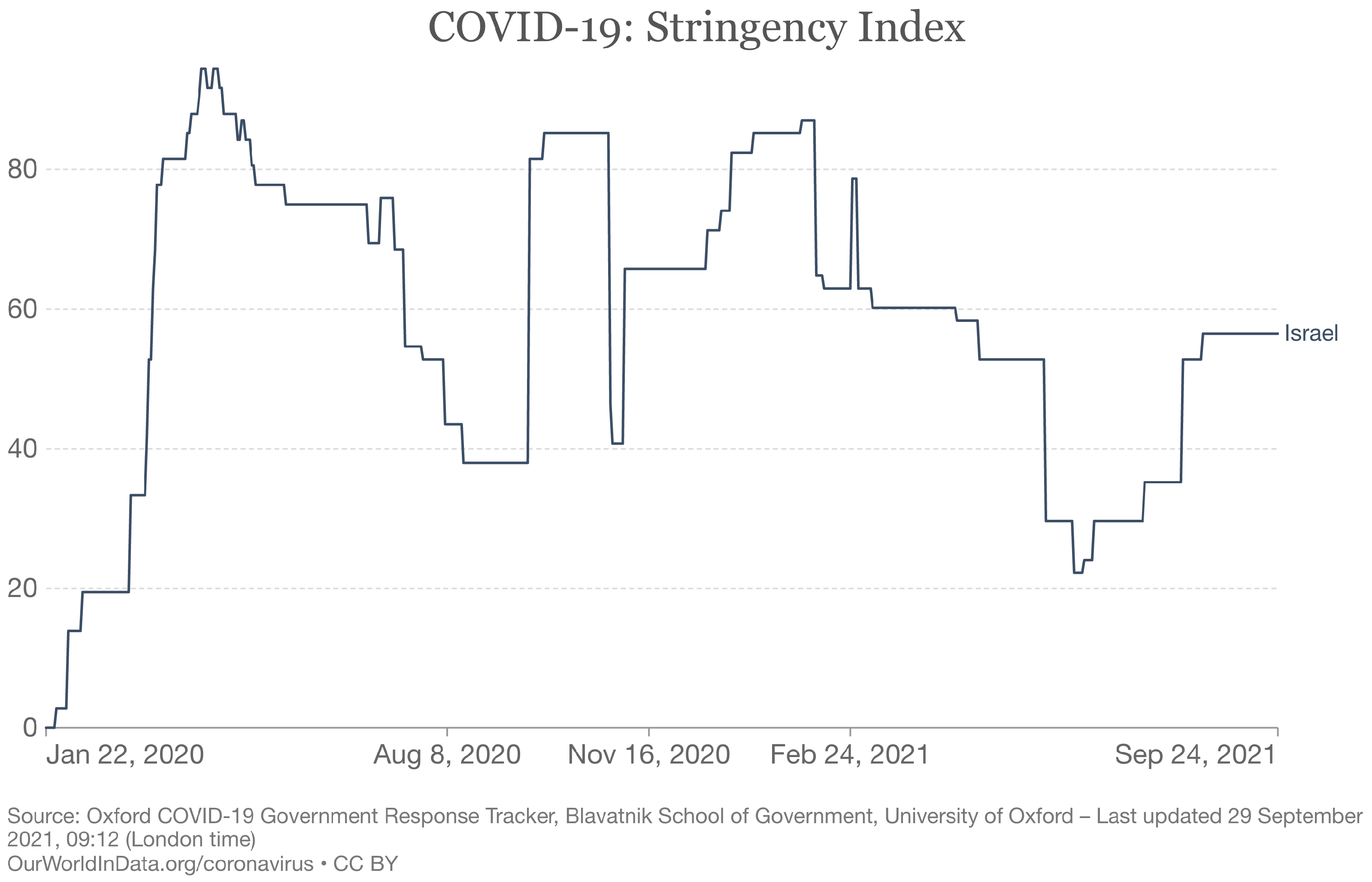
Figure 4.
Prior and posterior distributions of the model parameters.

Figure 5.
Comparison between the real-world data and the numbers of daily incidences obtained directly from our modified SEIR model. The fitted curve denotes the trajectory of with respect to date T. The scatter points specify the actual numbers of daily new cases over the ordered days of the outbreak. Note that has not contained the reporting delay D and the weekly modulation given in Equation (3), resulting in a smooth curve without noise.
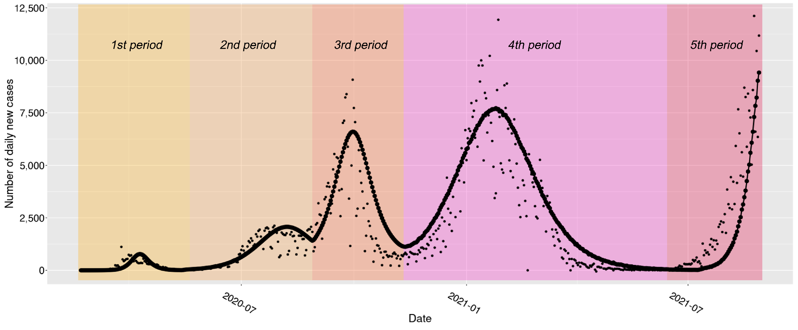
Figure 6.
Fitting and predicting the numbers of daily new cases. The fitted growth curve (dot-dashed) and the actual numbers (scatter points) of daily new cases over the ordered days of the outbreak. The predicted numbers of daily new cases (diamond shaped points with dashed lines) are demonstrated at the right side of the vertical line, which indicates the checkpoint of prediction (30 days before the end of study).

Figure 7.
The trajectories for cumulative cases. The fitted growth curve (dot-dashed) and the actual curve (solid line) of cumulative confirmed cases over the ordered days of the outbreak. The predicted numbers of cumulative cases (dot-dashed) are demonstrated at the right side of the vertical line, which indicates the checkpoint of prediction (30 days before the end of study).
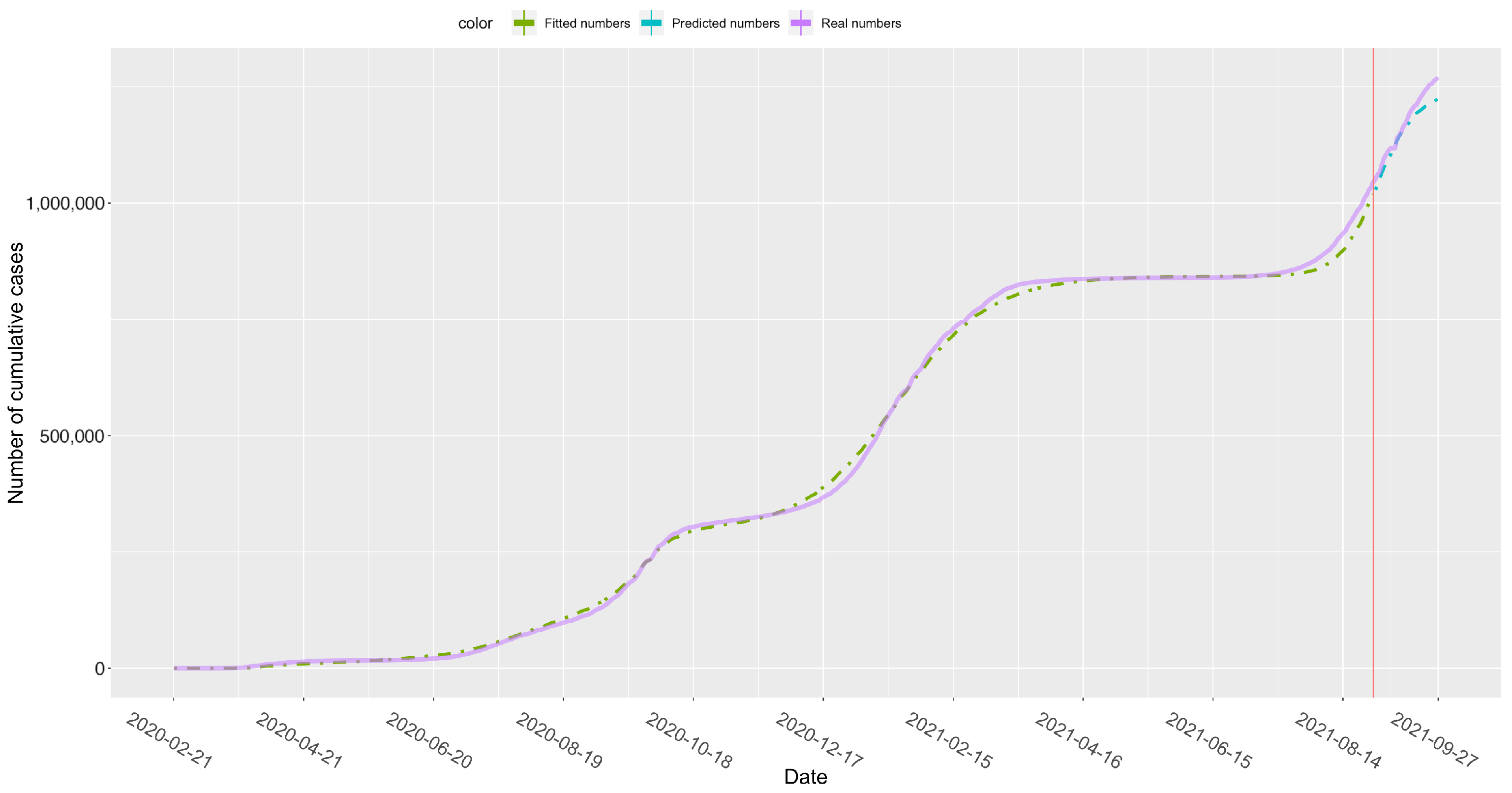
Figure 8.
Comparison between models. The fitted growth curve obtained from our modified SEIR model (solid diamond-shaped with dotted line) and the simulated growth curve yielded from the simpler model without vaccination (hollow star-shaped with dotted line) and the actual data (solid points) of daily confirmed new cases over the ordered days of the latest period (i.e., ). The simulated results from the simpler model show an overestimation of transmissibility along with a delayed prediction of the upcoming epidemic peak.


Table 1.
Priors on the model parameters.
| Parameter | Interpretation | Prior |
|---|---|---|
| Initial transmission rate | LogNormal(log(0.4), 0.5) | |
| Transmission rate after the 1st change point | LogNormal(log(0.4), 0.5) | |
| Transmission rate after the 2nd change point | LogNormal(log(0.4), 0.5) | |
| Transmission rate after the 3rd change point | LogNormal(log(0.4), 0.5) | |
| Transmission rate after the 4th change point | LogNormal(log(0.4), 0.5) | |
| Initial infectious rate | LogNormal(log(1/5), 0.5) | |
| Infectious rate after the 1st change point | LogNormal(log(1/5), 0.5) | |
| Infectious rate after the 2nd change point | LogNormal(log(1/5), 0.5) | |
| Infectious rate after the 3rd change point | LogNormal(log(1/5), 0.5) | |
| Infectious rate after the 4th change point | LogNormal(log(1/5), 0.5) | |
| Recovery rate | LogNormal(log(1/8), 0.2) | |
| D | Reporting delay | LogNormal(log(8), 0.2) |
| Initial number of infected | HalfCauchy(100) | |
| Initial number of exposed | HalfCauchy(100) | |
| The 1st change point | Normal(7 May 2020, 3) | |
| The 2nd change point | Normal(17 Aug 2020, 3) | |
| The 3rd change point | Normal(31 Oct 2020, 3) | |
| The 4th change point | Normal(20 Jun 2021, 3) | |
| Weekly modulation amplitude | Beta(4.39, 1.88) | |
| Weekly modulation phase | VonMises(0, 0.01) | |
| The proportion of cases reported | Beta(1, 2) | |
| Scale factor | HalfCauchy(10) | |
| Effective rate of the first dose | Normal(0.52,0.01) | |
| Effective rate of the second dose | Normal(0.95,0.01) |
Table 2.
Fitting results for model parameters and derived epidemiological parameters.
| Parameter | Mean | Standard Deviation | 95% Confidence Interval |
|---|---|---|---|
| 0.62 | 0.07 | [0.50, 0.76] | |
| 0.34 | 0.04 | [0.28, 0.45] | |
| 0.36 | 0.05 | [0.25, 0.45] | |
| 0.49 | 0.07 | [0.37, 0.64] | |
| 1.02 | 0.13 | [0.82, 1.31] | |
| 1.05 | 0.42 | [0.47, 2.09] | |
| 0.32 | 0.11 | [0.16, 0.59] | |
| 1.83 | 0.63 | [0.94, 3.35] | |
| 0.33 | 0.04 | [0.25, 0.42] | |
| 1.26 | 0.49 | [0.57, 2.45] | |
| 0.31 | 0.05 | [0.23, 0.41] | |
| D | 7.68 | 0.92 | [5.72, 9.30] |
| 1.51 | 1.87 | [0.05, 6.45] | |
| 1.59 | 2.02 | [0.04, 6.94] | |
| 8 May 2020 | 0.94 | [6 May 2020, 10 May 2020] | |
| 20 August 2020 | 0.68 | [19 August 2020, 22 August 2020] | |
| 1 November 2020 | 1.51 | [28 October 2020, 4 November 2020] | |
| 16 June 2021 | 1.63 | [13 June 2021, 20 June 2021] | |
| 0.58 | 0.06 | [0.47, 0.69] | |
| 3.71 | 2.72 | [1.74, 8.60] | |
| 0.20 | 0.01 | [0.18, 0.22] | |
| 19.79 | 0.89 | [18.11, 21.64] | |
| 0.52 | 0.03 | [0.47, 0.57] | |
| 0.95 | 0.01 | [0.93, 0.97] | |
| 2.03 | 0.24 | [1.64, 2.56] | |
| 1.10 | 0.01 | [1.07, 1.13] | |
| 1.17 | 0.04 | [1.11, 1.24] | |
| 1.59 | 0.04 | [1.50, 1.68] | |
| 3.33 | 0.32 | [2.79, 4.03] | |
| 1.10 | 0.43 | [0.48, 2.12] | |
| 3.50 | 1.14 | [1.70, 6.12] | |
| 0.61 | 0.20 | [0.30, 1.07] | |
| 3.11 | 0.40 | [2.38, 3.93] | |
| 0.91 | 0.35 | [0.41, 1.75] |
Publisher’s Note: MDPI stays neutral with regard to jurisdictional claims in published maps and institutional affiliations. |
© 2021 by the authors. Licensee MDPI, Basel, Switzerland. This article is an open access article distributed under the terms and conditions of the Creative Commons Attribution (CC BY) license (https://creativecommons.org/licenses/by/4.0/).
Share and Cite
MDPI and ACS Style
Xu, J.; Tang, Y. Bayesian Framework for Multi-Wave COVID-19 Epidemic Analysis Using Empirical Vaccination Data. Mathematics 2022, 10, 21. https://doi.org/10.3390/math10010021
AMA Style
Xu J, Tang Y. Bayesian Framework for Multi-Wave COVID-19 Epidemic Analysis Using Empirical Vaccination Data. Mathematics. 2022; 10(1):21. https://doi.org/10.3390/math10010021
Chicago/Turabian StyleXu, Jiawei, and Yincai Tang. 2022. "Bayesian Framework for Multi-Wave COVID-19 Epidemic Analysis Using Empirical Vaccination Data" Mathematics 10, no. 1: 21. https://doi.org/10.3390/math10010021
Note that from the first issue of 2016, this journal uses article numbers instead of page numbers. See further details here.