
Supply Chain Pricing Models Considering Risk Attitudes under Free-Riding Behavior


1
School of Management, Heilongjiang University of Science and Technology, Harbin 150027, China
2
School of Management, Harbin Institute of Technology, Harbin 150001, China
3
Heilongjiang Property Rights Trading Group, Harbin 150090, China
4
College of Letter & Science, University of California, Berkeley, CA 94720, USA
*
Authors to whom correspondence should be addressed.
Mathematics 2022, 10(10), 1723; https://doi.org/10.3390/math10101723
Submission received: 12 April 2022
/
Revised: 11 May 2022
/
Accepted: 16 May 2022
/
Published: 18 May 2022
(This article belongs to the Topic Game Theory and Applications)
Abstract
:The free-riding behavior of companies that do not act will bring losses to companies that provide services. A market consists of two secondary supply chains: manufacturers and retailers. Each supply chain can choose to adopt promotional strategies to expand its market demand. This paper constructs the centralized decision-making in the supply chain and the Nash game competition model between supply chains and primarily studies the impact of risk aversion and the free-riding coefficient on supply chain pricing, promotion strategy selection, and expected utility. We show that the supply chain with high-risk aversion has relatively low pricing, but the demand and a total expected utility are high. We also identify that, on the premise of the same risk aversion degree of the two supply chains, when the free-riding coefficient between the chains is small and equal, the supply chain tends to implement the promotion strategy. When consumers have the same preference for the products of two retailers, the pricing of the free-riding supply chain increases with the increase in the free-riding coefficient, while the supply chain with a promotion strategy is the opposite. Based on the numerical results, we further give the optimal one-way free-riding coefficient when the two supply chains have the same degree of risk aversion; when there is a bidirectional free-riding behavior in the market, competition among supply chains gradually tends to the first two scenarios.
1. Introduction
With the gradual improvement of the market and the increasing competition among companies, taking effective strategies to tap potential customers and expand market share is the key for companies to achieve sustainable development and remain invincible. One of the feasible strategies is that retailers can carry out some marketing activities to directly show consumers the characteristics of goods to promote sales, which is also a promotion strategy commonly used by most companies [1]. However, it will also bring some challenges to the promotion companies themselves [2].
On the one hand, the rapid development of e-commerce has broadened the retail channels of companies and brought many conveniences to consumers [3]. Owing to the homogeneity of products in both online channels and brick-and-mortar channels, consumers can choose purchasing channels according to their preferences [4,5]. However, in reality, some consumers tend to buy goods at a low price or equivalent through online channels after experiencing physical services through traditional brick-and-mortar channels [6]. According to some relevant surveys, if consumers can see the shape of products and understand their production process through some channels, nearly half (45%) of consumers tend to buy goods online [7]. Some traditional brand manufacturers have seized consumers’ purchasing preferences and opened online channels to expand their sales fields. For example, Apple, Huawei, Gome, and Suning have established online flagship stores for consumers to select and buy products online. At the same time, the opening of these enterprise network channels has promoted consumers’ online consumption. However, this phenomenon has had an impact on retailers who have not opened online channels. Therefore, even after the COVID-19 pandemic, consumers are still dependent on online channels, which is not conducive to the sales of brick-and-mortar channels [8]. For example, retailers that do not open online channels have sales losses, while the revenue of Amazon and other e-commerce companies has increased significantly [9].
On the other hand, because of the homogeneity of products sold by retailers in the same industry, when some companies make efforts to promote their products, inactive companies indirectly enjoy the convenience brought by promotional companies. For example, when consumers’ demand for innovative enterprise products increases, the total demand for similar products will also increase at the same time because many consumers prefer to buy imitations or substitutes of brand products [10]. Midea’s promotion of variable frequency air conditioners will encourage consumers to buy Gree variable frequency air conditioners, but this behavior of inactive retailers will weaken the enthusiasm of companies’ investment promotion strategy and reduce the overall benefits of each supply chain.
Interestingly, these two phenomena have one thing in common: the companies can benefit from competitors’ services or strategies without paying any cost, thus affecting the optimal decision-making of each enterprise and the total revenue of the supply chains. This service or strategy spillover effect is called “free-riding” behavior [11] or “exhibition hall phenomenon” [6]. Simply, in daily life, “just looking but not buying” is typical free-riding behavior. Although consumers accept the marketing services of their sales associates in a retail store to understand the products, they will eventually buy the same products at different stores or channels. In addition, there is another free-riding situation where some consumers visit online stores to learn more about product quality, price, after-sales service, and so on. Next, they will choose intuitive brick-and-mortar stores after comparison [12]; Jingdong Mall first launched the “6.18” special mid-year promotion activity in 2008, and Taobao launched the “double 11” hot sale activity in 2009. At this time, these two platforms competed with each other as independent companies, but Taobao also joined the Jingdong Mall store festival in 2015. Until now, Jingdong and Taobao are still promoting each other on each other’s platforms on their specific activity day, which shows that there is mutual free riding between companies in the market. However, the bidirectional free-riding behavior is different from the one-way free-riding behavior [13]. Thus, the study of free-riding behavior plays an important role in helping companies make decisions in pricing and sales.
Many previous studies on free-riding behavior have mainly focused on the situation that network channels take free-riding service from brick-and-mortar channels in the dual-channel supply chain and studied the pricing strategies and service levels of companies from the perspective of consumer free riding. However, free-riding behavior is also common among network channels and brick-and-mortar channels, and with the intensification of market competition and complex and changeable demand, the competition among companies gradually rises to the competition among supply chains. In addition, most companies only aim to reduce the expected cost or improve the expected profit while ignoring the risk preference of decision-makers. Because of the complexity and variability of the market demand, supply chain members must face uncertain risks, which will affect product price [5], inventory [14], the expected demand [15], and other decisions. To improve the efficiency of the supply chain, companies pay more and more attention to incorporating risk control into decision making, so it is crucial to consider risk control and decision-makers’ risk preference in the decision-making process [16]. Companies further make decisions by maximizing their target utility function according to their risk attitudes. Since risks have an impact on all links of the supply chain, it is more scientific to consider the overall risk attitudes of the supply chain. Therefore, this paper attempts to supplement the existing research by solving the following problems:
- (1)
- At what value are the free-riding coefficient, the pricing, and profit of the supply chain with a promotion strategy optimal;
- (2)
- How does the supply chain with a promotion strategy deal with the risks brought by free-riding behavior between supply chains;
- (3)
- When all supply chains implement promotion strategies at the same time, how to analyze the impact of the bidirectional free-riding behavior between supply chains on the pricing and profit of each supply chain?
The main contributions of this paper are as follows: (1) This paper extends the free-riding problem of the dual-channel supply chain to a more general case. It focuses on the decision-making problem between supply chains under the free-riding behavior of two supply chains producing homogeneous products in the market and finds the optimal one-way free-riding coefficient, which is different from the method of [17,18,19]. (2) We integrate free-riding behavior into the supply chain risk model and study the optimal pricing and total expected utility of each supply chain under different circumstances, which is different from the method of [20,21,22]. (3) This paper further examines the bidirectional free-riding problem between supply chains, which is different from the method of [23,24,25].
The rest of this study will be described in the following order. In Section 2, we review the relevant literature. Section 3 describes the model and puts forward relevant assumptions. On this basis, we construct four models and deduce the equilibrium solutions. Section 4 presents the numerical analysis. Finally, we conclude the paper in Section 5. The expressions of some capital letters in the paper are shown in Appendix A.
2. Literature Review
Two fields of previous studies are relevant to this study: free-riding behavior and risk attitudes. Among them, the literature research on free-riding behavior is discussed from three aspects: positive impact, negative impact, and both. In this section, we review the relevant literature.
2.1. Positive Impact of Free-Riding Behavior
The positive impact of free-riding behavior refers to the benefits of free-riding behavior of companies or consumers in the market to themselves or supply chain members. In this course, Shin [20] believed that consumers’ free-riding behavior weakens the price competition between retailers, which can be beneficial to all nodes of the supply chain. Liang and Sun [21] believed that the proper degree of service free-riding can increase the greening of the dual-channel supply chain. Wang et al. [22] investigated the impact of different data values generated by two service providers and one service integrator on member pricing and profit based on the digital background. They found that service integrators as leaders could gain more utilities at no cost through free riding. Jing [26] and Liu et al. [27] investigated the exhibition hall effect of the brick-and-mortar channel and the network channel. They found that free-riding behavior is conducive to improving product matching. Yan et al. [28] further discussed the optimal pricing, sales efforts, market demand, and other problems of members under no free-riding behavior, one-way free-riding, and bidirectional free-riding by developing a dual-channel supply chain model between one traditional retailer and one e-commerce platform led by retailers. They prove that the bidirectional free-riding behavior of traditional retailers and e-commerce platforms under online finance can increase not only the profits of participants but also expand the total market demand of the supply chain.
2.2. Negative Impact of Free-Riding Behavior
However, the negative impact of the free-riding behavior of consumers or companies on other companies is more obvious. In this course, Mittelstaedt [29] and Chiou et al. [30] found that free-riding behavior weakens the enthusiasm of service retailers. Zheng and Bao [31] established a Cournot game competition model, including one manufacturer and two retailers producing alternative products, to study the business decision-making of each member. They found that the joint investment intention of the two retailers decreased with the increase in the free-riding coefficient caused by the product spillover effect. Ke and Jiang [32] constructed the free-riding model between one manufacturer and two retailers, and the free-riding model between two retailers under the leadership of the manufacturer and retailer, respectively. They investigated the marketing efforts and decisions of members under different models. They found that the more serious the free-riding phenomenon, the more reluctant the dominant retailers are to make marketing efforts. Free-riding behavior will not only reduce the enthusiasm of companies to make efforts but also reduce their profits. Balakrishnan et al. [33] and Jing [26] studied the impact of consumers’ free-riding behavior on the price competition between online retailers and brick-and-mortar retailers under the dual-channel supply chain structure. They found that free riding will aggravate the price competition among them and reduce the profits of brick-and-mortar retailers. Liu et al. [34] constructed the differential game model of two competitive companies under the consideration of enterprise foresight and shortsightedness, examined their pricing decision and innovation investment strategy and found that when the two companies’ behaviors are different, the free-riding behavior of short-sighted companies will occur. When the cross innovation investment demand sensitivity coefficient between the two companies is small, the profit of short-sighted companies is higher than that of long-sighted companies. Based on the premise of supplier green investment, Wang et al. [35] discussed the investment strategy of e-retailers and found that e-retailers prefer to take the free riding of supplier investment, and this behavior can increase their income but damage the interests of suppliers.
In addition, some solutions to this conflict based on the free-riding problem have been given by some scholars. Considering that online retailers take the sales efforts of brick-and-mortar retailers for free, Xing and Liu [36] studied the coordination of sales efforts among them and found that the free-riding behavior of online retailers not only weakens the expected effort level of brick-and-mortar retailers but also damages the overall utility of upstream companies and supply chain. They designed a contract with price matching and optional compensation rebates to coordinate sales efforts. Considering the free-riding behavior of consumers, Pu et al. [37] established a dual-channel supply chain decision-making model. They found that under deterministic demand, regardless of centralized or decentralized model, the sales effort level of brick-and-mortar stores and total profit of the supply chain changes inversely with the number of consumers’ free riding. However, manufacturers tend to actively put forward cost-sharing contracts to promote brick-and-mortar stores to provide sales efforts to achieve a win-win situation. Based on the limited rationality of manufacturers and suppliers, Sun et al. [38] studied the green investment strategies of both sides under different subsidy mechanisms by constructing an evolutionary game model and found that appropriate government subsidy can reduce the free-riding behavior among both sides in the market.
2.3. The Double-Sided Nature of Free-Riding Behavior
In addition to the above research, partial scholars have found that there are two sides to the free-riding behavior of consumers or companies. Zhang et al. [23] established a differential game model to investigate the dynamic green innovation decision making among the green innovative manufacturers, a free-riding manufacturer, and green suppliers. The research showed that the profits of the innovative manufacturer are always lower than the free-riding manufacturer, and the supplier’s technology spillover can increase the profit gap between the innovative manufacturer and the free-riding manufacturer, but the technology spillover of the innovative manufacturer has the opposite impact. Based on the fact that the manufacturer’s online channel and the retailer’s traditional channel share the retailer’s pre-sales service cost, Zhou et al. [24] studied the impact of consumers’ free-riding behavior on dual-channel differential and nondifferential pricing, service strategy, and profit, and found that free riding always hurts the retailer’s profit, but has a positive impact on the manufacturer’s and the whole supply chain’s profit. He et al. [25] analyzed the impact of free-riding behavior on product carbon emissions by developing a closed-loop supply chain model including one remanufacturer, one traditional retailer, and one e-retailer. The research result showed that, although consumers’ free-riding behavior may bring benefits to the remanufacturer, it also increases the total carbon emissions of the supply chain. Xu and Wang [39,40] examined the investment decision making in carbon emission reduction under centralized and decentralized decision-making by building a two-level Stackelberg model led by suppliers and led by manufacturers. They found that technology spillover amplifies the impact of free-riding behavior, and with the increase in technology spillover, the carbon emission and profit of each member of the supply chain gradually increase, but the price of parts and finished products is the opposite. Additionally, Liu et al. [41] further applied the customer utility theory to develop a dual-channel supply chain pricing model with or without free-riding behavior. They found that although consumers’ free-riding behavior can increase the total market demand by affecting the pricing decisions of members, it also exacerbates the conflict between channels, thus reducing the profits of retailers and improving the profits of manufacturers.
2.4. Risk Attitudes
In the process of operations, companies often face many challenges, such as market uncertainty risk, natural environment risk, policy risk, and so on. However, different companies have different risk attitudes and market returns. Individual risk attitudes may be a core dimension behind various social and economic decisions [42], influencing how participants adjust their level of cooperation in light of the new social environment [43]. Taking the value-at-risk criterion as the risk evaluation standard, Zhu et al. [17] investigated the decision-making model of risk-averse retailers in the dual-channel supply chain under supply and demand uncertainty and proposed a joint contract to achieve Pareto improvement of supply chain performance. Sun et al. [16] considered the volatility of consumer demand and studied the impact of decision-making factors, such as the wholesale price, on the average utility of each node under the risk-averse attitudes of all participants in the supply chain. In addition, Xu et al. [5] discussed the channel coordination between risk-averse manufacturers and retailers in a dual-channel supply chain based on the mean-variance model. Li et al. [18] and Jiang et al. [19] further considered that the market comprises one risk-averse retailer and one risk-neutral supplier under demand uncertainty and studied the coordination of channel pricing, demand, and profit in the dual-channel supply chain. They proposed a new risk-sharing contract to achieve synergy among members. However, Ma et al. [44] designed a Nash negotiation mechanism for pricing and order quantities for risk-averse retailers and risk-neutral suppliers. Li et al. [45] further constructed the dual-channel Nash game model of the two. They found that the retailer’s price is inversely proportional to its risk aversion degree under the uncertainty of demand. Zhao et al. [15] examined the impact of risk attitudes on the expected demand and income of remanufacturers and retailers and put forward corresponding strategies to solve the balance between expected income and market fluctuation risk. Based on the literature, Xu et al. [46] discussed the impact of free-riding behavior on inventory, ordering, and sales efforts in decentralized and centralized supply chains under random demand based on the risk-neutral attitude of manufacturers and retailers. Considering the risk attitudes of brick-and-mortar retailers, Ma and Hong [47] established static and dynamic game models on retailer pricing and service strategy under the dual-channel structure based on the mean-variance theory. They found that the service level of brick-and-mortar retailers is directly proportional to their risk preference, but their price and service level are inversely proportional to the free-riding behavior of online channel retailers.
In summary, although previous scholars have conducted systematic research on free-riding behavior, most previous studies have only discussed the problem of one-way free-riding. Less research has been carried out on bidirectional free-riding behavior and only considered one side risk aversion, one side risk neutrality [19,44,45], or both complete risk aversion in the manufacturers and retailers in the supply chain [5,16]. However, free-riding behavior may increase the profits and market demand of both sides [28] and also aggravate the price competition of companies [26,33]. At the same time, companies may have different risk attitudes in different situations, which may be positive or negative [48]. Hence, different from the literature, from the perspective of the supply chain, this paper contrasts and analyzes the impact of the free-riding coefficient and different risk aversion degrees of the two supply chains on supply chain decision making in the case of no free-riding behavior, one-way free-riding, and bidirectional free-riding, to supplement the research in this field.
3. The Model
3.1. Model Description
Considering that the market is composed of two supply chains producing homogeneous products: supply chain 1 (SC1) and supply chain 2 (SC2), each supply chain contains one manufacturer and one retailer, and the retailer and the manufacturer in the chain fully cooperate and share information as a whole, to make centralized decisions to maximize the profits of the supply chain, and jointly determine the cost-sharing proportion of supply chain promotion. The power of the two supply chains is equal, and the Nash game and simultaneous decision making are carried out between the supply chains. Among them, each supply chain can tap potential customers and expand market demand through the implementation of a promotion strategy, but the implementation of a promotion strategy will produce corresponding effort costs and cause the free-riding behavior of another supply chain. When the two supply chains choose to implement the promotion strategy at the same time, it will lead to the bidirectional free-riding behavior between the supply chains. Therefore, for both supply chains, the market has the risk of demand uncertainty and the risk of loss of benefits. Under this background, the two supply chains compete on whether to implement a promotion strategy in the market or not. The model framework is shown in Figure 1.
3.2. Notation Definition and Model Assumptions
According to the foregoing, the variables and notations required for the study are shown in Abbreviation.
Among them, , , follow the normal distribution, i.e., ; the effort cost of supply chain implementing promotion strategy is [24,49].
To more clearly describe the research problems, this paper also makes the following assumptions:
- (1)
- The potential market demand is large, and when consumers have the same preference for the two products, the demand meets ;
- (2)
- The implementation of a promotion strategy in the supply chain can expand its market demand and increase potential customers. At the same time, it will produce free-riding behavior between supply chains [50]. The increased income of free-riding companies is not necessarily less than that of companies implementing promotion strategies;
- (3)
- Consumers choose to buy merchants mainly based on their own needs and time cost, which is less affected by the cross-price elasticity coefficient between supply chains, i.e., [51];
- (4)
- It is assumed that the wholesale price of products provided by manufacturers to retailers in the two supply chains is equal and unchanged; the unit production cost of the two manufacturers is the same, which is , and the unit sales cost and each sunk cost of the retailer are not considered;
- (5)
- According to the mean-variance theory, the total expected utility of the supply chain is composed of its expected profit and standard deviation, that is: [15,52], where indicates that the supply chain is completely risks neutral, indicates that the supply chain is completely risk-averse and the greater the is, the more risk-averse the supply chain is [16].
3.3. Model Construction
3.3.1. Neither Supply Chain Implements a Promotion Strategy
In this case, the two supply chains compete fairly in the market, and the total expected utility of the supply chain mainly depends on the risk aversion degree of each supply chain. This section can be used as a benchmark for the remaining three cases. According to the above assumptions and the models constructed by Chiou et al. [30], Zhou et al. [24], Sun and Ma [16], and Huang and Swaminathan [51], the market demand functions of the two supply chains can be assumed as and , so then the manufacturer’s expected profit is , and the retailer’s expected profit is . Considering the risk aversion degree of the supply chain, the total expected utility of supply chain SC1 is:
The total expected utility of supply chain SC2 is:
Find the partial derivative of Equation (1) concerning and Equation (2) concerning . According to the foregoing, , so , . Simultaneous and can obtain the unique Nash equilibrium solution, in this case, that is, the optimal pricing of SC1 is:
The optimal pricing of SC2 is:
Substituting Equations (3) and (4) with Equations (1) and (2), the optimal total expected utility of each supply chain can be obtained.
Proposition 1.
When, then; when, then .
Proof.
Subtract from Equations (3) and (4): . It can be seen from Equation (3) that . Additionally, according to the above assumptions, . So when , then ; when , then , the certificate is completed. □
Proposition 1 shows the state when consumers have the same preference for the products of the two retailers, and the market demand is greater than a certain threshold: when the risk aversion degree of SC2 is greater than SC1, its price is less than the retail price of SC1; when the risk aversion degree of SC2 is less than SC1, its price is greater than the retail price of SC1, which also shows that in the fair competition market, the supply chain with high-risk aversion has weak risk tolerance and response ability and is more inclined to adopt conservative strategies, that is, the price is lower than that of competitors.
3.3.2. SC2 Promotes Promotion Strategy and SC1 One-Way Free Riding
In this case, SC2 adopts a promotion strategy to expand market demand, but SC1 provides homogeneous products and faces the same market, which will produce free-riding behavior between supply chains: SC2 promotes the promotion strategy with effort level , and SC1 gives a free-riding in the market with . At this time, the total expected utility of the supply chain mainly depends on the degree of risk aversion and free-riding coefficient. Therefore, SC1 and SC2 demand functions can be expressed as: and , respectively. At this time, the expected profit of the SC1 manufacturer is: ; the retailer’s expected profit is: . In addition, the manufacturer and retailer in SC2 bear the promotion costs with and , respectively, so the expected profit of the SC2 manufacturer is: ; the retailer’s expected profit is: . Considering the risk aversion degree of the supply chain, the total expected utility of SC1 is:
SC2 total expected utility is:
Find the partial derivative about for Equation (5) and the partial derivative about for Equation (6). Since the second-order partial derivatives are less than 0, the only Nash equilibrium solution, in this case, can be obtained by combining the first-order partial derivatives. The optimal pricing of SC1 and SC2 are, respectively (see the Appendix A for capital letters in the equations):
Subsuming Equations (7) and (8) into Equations (5) and (6) can obtain the optimal total expected utility of each supply chain. Because is a strictly concave function for , let its first partial derivative be equal to 0, and the optimal effort level when SC2 implements the promotion strategy is:
Proposition 2.
,.
Find the partial derivative of Equations (7) and (8) for , and get: , , so , . Proposition 2 shows that the retail prices of SC1 and SC2 are in direct proportion to the effort level of SC2 to implement the promotion strategy. For SC2, the promotion strategy is beneficial to explore potential customers, and , so the increase in effort level leads to the increase in market demand and the retail price of SC2 increases accordingly. For SC1, exists, that is, when SC2 improves its effort level to expand market demand, SC1 indirectly shares part of the potential market because of the free-riding behavior between supply chains, thus increasing the retail price of SC1.
Corollary 1.
Based onand the same consumer preference for the two products, supply chain SC2 tends to implement promotion strategy only when.
Proof.
When the risk aversion degree of the two supply chains is the same, the first-order partial derivative about is obtained from Equations (7) and (8) and subtracted to obtain: , and , . From the above, we know that , so when , then , , ; when , then , , ; when , then , , , the certificate is completed. □
From the above proof process, it is known that on the premise of the same degree of risk aversion of the two supply chains and the same consumer preference for the products of the two retailers, the market demand and optimal pricing of the two supply chains differ in their sensitivity to the one-way free-riding coefficient between the supply chains and SC2 effort level. If and only if , both the market demand and optimal pricing of SC2 are greater than that of SC1. At this time, the rational supply chain SC2 tends to make efforts to implement the promotion strategy; otherwise, SC2 is unwilling to implement the promotion strategy.
Proposition 3.
, .
Proof.
Find the partial derivatives of the first order of Equations (7) and (8) concerning and we can be obtained as follows: , and , and , so , , the certificate is completed. □
Proposition 3 shows that when SC2 makes efforts to implement the promotion strategy, because of the free-riding behavior between supply chains, SC1 retail price increases with the increase in the free-riding coefficient, while SC2 retail price decreases with the increase in the free-riding coefficient. Horizontal comparison of the pricing and market demand of each supply chain shows that, although the retail price of SC2 is inversely proportional to the one-way free-riding coefficient between the supply chains, the promotion strategy of SC2 can expand the market demand of both, and the price is higher than that when neither of them implements the promotion strategy. SC2 makes efforts to implement the promotion strategy when and only when the free-riding coefficient reaches .
Proposition 4.
, .
From the expected profit function of SC2 manufacturers and retailers, it is obvious that , . The proposition shows that the manufacturer’s expected profit is inversely proportional to the proportion of promotion cost, while the retailer’s expected profit is the opposite. Obviously, rational companies, manufacturers, and retailers want each other to bear more promotion cost-sharing proportion. Therefore, when the downstream retailers are monopolized, there is no optimal promotion cost-sharing proportion in the supply chain that makes the expected profit function of manufacturers and retailers reach the optimal promotion cost-sharing proportion at the same time.
If SC2 implements the promotion strategy so that the expected profits of its manufacturers and retailers are higher than that in the first case, there is an acceptable promotion cost-sharing proportion for SC2 manufacturers and retailers, that is, Proposition 5.
Proposition 5.
If, then there is a value range of:, which is the promotion cost-sharing proportion acceptable to both manufacturers and retailers.
Proof.
Let . It can be seen from the above that and . Let , . If , then , then and are further obtained, so is the proportion of promotion cost sharing acceptable to both manufacturers and retailers. □
In the Proposition 5, represents the maximum promotion cost-sharing proportion acceptable to the manufacturer, and represents the minimum promotion cost-sharing proportion acceptable to the retailer. Therefore, under the centralized decision-making, SC2 manufacturer and retailer can determine their promotion cost-sharing proportion through negotiation, which can not only increase the total expected utility of the supply chain but also improve the expected profits of both parties. When the manufacturer observes that the retailer’s level of efforts to improve the promotion strategy can increase the total expected utility of the supply chain, it will negotiate with the retailer and design a mechanism to reasonably allocate the total expected utility of the supply chain, to promote the retailer to improve the level of promotion efforts, and realize the Pareto optimization of the total expected utility of the supply chain.
Proposition 6.
Under Rubinstein’s bargaining model, there exists an optimal Pareto promotion cost-bearing ratio.
In the allocation of promotion cost, the manufacturer of SC2 tends to value closer to , while the retailer tends to value closer to . Meanwhile, the manufacturer and the retailer hope to obtain more additional expected utility, so the Rubinstein bargaining model is adopted to solve the distribution problem of expected utility outside the total amount of the supply chain. Rubinstein believes that in the infinite exchange bidding game, there is a unique subgame refined equilibrium between the two sides, where and represent the discount factor (patience) of the manufacturer and the retailer, respectively, keeping other conditions unchanged so that the party with high patience can get more shares [53].
It can be seen from the above that . Given and , the optimal additional expected utility obtained by the manufacturer and the retailer, respectively, can be obtained from the Rubinstein bargaining model: and . Therefore, the optimal Pareto promotion cost-bearing ratio of the manufacturer and the retailer is: . Combined with proposition 5, we can get: . Find the first-order partial derivatives of concerning and respectively, then get and . Therefore, when the manufacturer’s patience decreases or the retailer’s patience increases, the optimal Pareto promotion cost-bearing proportion will increase.
The solution process of the optimal promotion cost-sharing ratio in the following two cases is similar to the second case, which will not be discussed in detail.
3.3.3. SC1 Promotes Promotion Strategy and SC2 One-Way Free Riding
In this case, SC1 adopts a promotion strategy to expand market demand, but SC2 provides homogeneous products and faces the same market, which will produce free-riding behavior between supply chains. SC1 promotes the promotion strategy with effort level , and SC2 gives a free riding in the market with . At this time, the total expected utility of the supply chain mainly depends on the degree of risk aversion and free-riding coefficient. Then SC1 and SC2 demand functions can be expressed as and respectively; the expected profits of manufacturers and retailers of SC2 can be expressed as and , respectively. In addition, if the manufacturer and retailer in SC1 bear the promotion cost with and , respectively, the expected profit of the SC1 manufacturer is , and the expected profit of the retailer is . Considering the risk aversion degree of the supply chain, the total expected utility of SC1 is:
SC2 total expected utility is:
Find the partial derivative concerning for Equation (10) and the partial derivative concerning for Equation (11). Since the second-order partial derivatives are less than 0, the only Nash equilibrium solution, in this case, can be obtained by combining the first-order partial derivatives; that is, the optimal pricing of SC1 and SC2 are, respectively (see the Appendix A for capital letters in the equations):
By subsuming Equations (12) and (13) into Equations (10) and (11), the optimal total expected utility of each supply chain can be obtained. Since is a strictly concave function concerning , let the first partial derivative be equal to 0, then the optimal effort level of SC1 in promoting promotion strategy is:
3.3.4. Both Supply Chains Carry out Promotion Strategies, Resulting in Bidirectional Free-Riding Behavior
In this case, SC1 and SC2 adopt promotion strategies to expand market demand at the same time, which will produce a bidirectional free-riding behavior between supply chains: SC1 and SC2 not only implement promotion strategies at the effort level and , respectively, but also free-riding at the level of and , respectively, in the market. Then the market demand function of SC1 is , and the market demand function of SC2 is . In addition, manufacturers and retailers in SC1 and SC2 bear the promotion costs with and , respectively, so the expected profits of manufacturers and retailers in the two supply chains are and , respectively. Considering the risk aversion degree of the supply chain, the total expected utility of SC1 is:
SC2 total expected utility is:
Find the partial derivative concerning for Equation (15) and the partial derivative concerning for Equation (16). Since the second-order partial derivatives are less than 0, the only Nash equilibrium solution, in this case, can be obtained by combining the first-order partial derivatives; that is, the optimal pricing of SC1 and SC2 are, respectively (see the Appendix A for capital letters in the equations):
Subsuming Equations (12) and (13) into Equations (10) and (11) can obtain the optimal total expected utility of each supply chain. Calculating the first-order partial derivatives of Equations (15) and (16) concerning and , and making them equal to 0, we can obtain the respective optimal effort level of the two supply chains in this case:
4. Numerical Experiments
To further verify the rationality and effectiveness of the model and the internal relationship between explanatory variables, in this section, we will use a numerical example to study the impact of the free-riding coefficient between supply chains and the degree of risk aversion on the pricing, promotion strategy effort level, market demand, and total expected utility of the two supply chains. Concerning the variable setting in reference [34], and after making appropriate adjustments to some variables, the values of some variables are set as follows: , , , , , and .
4.1. Influence of the Degree of Risk Aversion on Expected Demand and Total Expected Utility of Supply Chains under No Free-Riding Behavior
Given that changes within the range of [0,1] and the step size is 0.1, it is analyzed whether the expected demand and total expected utility of the two supply chains change with the degree of risk aversion in the first case. The results are shown in Figure 2.
According to Figure 2:
- (1)
- Both supply chain risk aversion coefficients have an impact on SC1 expected demand and total expected utility, but the impact of is more significant, indicating that the supply chain is more sensitive to the change in its risk aversion degree;
- (2)
- The expected demand of SC1 changes positively with and negatively with , because as the degree of SC1 risk aversion increases, gradually decreases according to proposition 1, and price reduction is beneficial to expand the market demand of SC1 under the condition of homogeneity of products and the same market. Similarly, keeping the unchanged, with the increase in , the market demand for SC2 increases, and the market demand for SC1 decreases accordingly;
- (3)
- The total expected utility of supply chain 1 and the risk aversion coefficient of the two supply chains change in the opposite direction. Although the market demand for SC1 changes positively with , , that is, the impact of price reduction is greater than that of demand increase. Lower risk tolerance leads to a smaller total expected utility, and when , the total expected utility of SC1 is the largest, which also reflects the principle of high risk and high return. Similarly, we can see from the fact that SC2 pricing decreases with the increase in its degree of risk aversion, SC2 market demand increases accordingly, and SC1 will tend to adopt a price reduction strategy with higher risk aversion to maintain the same competitiveness, so gradually decreases. The changes in total expected utility and expected demand of supply chain SC2 are similar to this section and will not be discussed here.
4.2. Influence of the Degree of Risk Aversion on Each Variable
When a supply chain makes efforts to implement the promotion strategy, it will cause the free-riding behavior of another supply chain on the premise of product homogeneity. Firstly, assuming that the free-riding coefficient , and the risk aversion degree and take 0.2, 0.5, and 0.8, respectively, we analyze the impact of the risk aversion degree of the two supply chains on the pricing, effort level, and total expected utility of the supply chains, as shown in Table 1, Table 2 and Table 3. Then, assuming the free-riding coefficient and , we analyze the impact of the risk aversion degree of the two supply chains on pricing and total expected utility in the second case, as shown in Table 4.
- (1)
- As for the degree of risk aversion of a single supply chain, in any case, the pricing, effort level, and total expected utility of the supply chain are inversely proportional to the degree of risk aversion of itself and the other supply chain. This shows that when the degree of risk aversion of either supply chain increases, both supply chains in the market tend to adopt a conservative strategy, that is, reducing the price. However, it is known from 4.1. that the impact of price reduction is greater than that of demand increase, so the effort level and total expected utility of the supply chain are reduced accordingly;
- (2)
- When the degree of risk aversion of the two supply chains is the same, the pricing, effort level, and total expected utility of the supply chain are the largest when both supply chains implement the promotion strategy, the second when a single supply chain implements the promotion strategy, and the smallest when neither supply chain implements the promotion strategy. When the two supply chains adopt the same strategy, they have the same pricing, the same effort level, and the same total expected utility of the supply chain. When the two supply chains adopt different strategies, the supply chain pricing, effort level, and total expected utility of the promotion strategy are higher. This shows that under the same degree of risk aversion of the two supply chains and the small and equal free-riding coefficient between the supply chains, the promotion strategy of any supply chain can increase potential customers, expand the market demand of both sides, and further promote the supply chain to improve the effort level, pricing, and total expected utility. When both sides choose to implement the promotion strategy, each variable reaches the best result;
- (3)
- When the degree of risk aversion of the two supply chains is different, no matter what strategies they adopt, the pricing and total expected utility of the supply chain with a higher degree of risk aversion are lower, and the pricing and total expected utility of the supply chain with a lower degree of risk aversion are higher, which also reflects the principle of high risk and high return, and has nothing to do with whether the supply chain implements the promotion a strategy or not and the free-riding coefficient.
- (4)
- According to Table 1, Table 2 and Table 4, on the premise of an equal free-riding coefficient and the same degree of risk aversion in the supply chain, if the one-way free-riding coefficient between the supply chains is small, the supply chain pricing and total expected utility of the promotion strategy are higher than that of the other party. Otherwise, it is beneficial to the supply chain without a promotion strategy and has nothing to do with the risk aversion degree of the supply chain. This shows that only when the free-riding coefficient is small the promotion strategy is beneficial to itself, which further verifies the corollary 1 conclusion. At the same time, it shows that there is a critical value of a one-way free-riding coefficient between 0.2 and 0.5, which makes the total expected utility of the two supply chains equal. The analysis processes of SC1 implement promotion strategy and SC2 one-way free riding, two supply chains implement promotion strategy at the same time, and common free-riding are similar to the second case and will not be discussed here.
The following research further analyzes the impact of the change of the free-riding coefficient on various variables and finds the optimal one-way free-riding coefficient under a certain degree of supply chain risk aversion. Assuming , which indicates that both supply chains have certain risk tolerance.
4.3. Impact of Variation of the One-Way Free-Riding Coefficient on Various Variables
According to corollary 1, only when the free-riding coefficient between supply chains changes within the range of [0,0.5] does the supply chain tends to make efforts to implement the promotion strategy. Therefore, when changes within [0, 0.5] and the step size is 0.01, we analyze the impact of the change of the one-way free-riding coefficient on the optimal pricing, expected market demand, the total expected utility of the two supply chains, and optimal effort level in the second case, as shown in Figure 3 and Figure 4.
- (1)
- The optimal effort level of SC2 changes inversely with the one-way free-riding coefficient between the supply chains, which means that the greater the free-riding coefficient, the less inclined SC2 is to make efforts to implement the promotion strategy. This reduces the enthusiasm of the supply chain to implement the promotion strategy and is not conducive to expanding the market demand of both sides;
- (2)
- When , the market demand and retail price of SC2 are always greater than that of SC1, and only when , the market demand and optimal pricing of the two supply chains are equal, which also indicates that when the free-riding coefficient between supply chains is small, rational SC2 will make efforts to implement promotion strategy; otherwise it will not adopt promotion strategy;
- (3)
- The total expected utility of SC1 increases with the increase in the free-riding coefficient, and the total expected utility of SC2 decreases with the increase in the free-riding coefficient. Only when , they are equal. This is because, although and , the increase in the free-riding coefficient between supply chains gradually makes the total expected utility of the two consistent, and when , , which further shows that when , SC2 makes efforts to promote the promotion strategy beneficial to it. The conclusion of the third case is similar to this and will not be discussed here.
4.4. Impact of Variation of the Bidirectional Free-Riding Coefficient on Various Variables
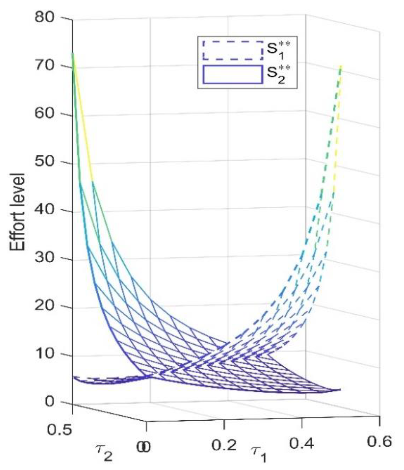
The simultaneous promotion strategy of the two supply chains will produce a bidirectional free-riding behavior between the supply chains. As is known above, we will analyze the impact of simultaneous change of both free-riding coefficients on each variable in the fourth case, as shown in Figure 5, Figure 6 and Figure 7.
- (1)
- When the two supply chain hitchhiking coefficients are not equivalent, the pricing, effort level, and total expected utility of the supply chain with a large coefficient are greater than those with a small coefficient. When the bidirectional free-riding coefficient takes or , the value of each variable reaches the maximum. This shows that when the free-riding coefficients of the two supply chains are different, the supply chain with a larger coefficient has an advantage in the market, and the supply chain with a competitive disadvantage may choose not to implement a promotion strategy. The competition gradually turns into the second or third case, which is not conducive to improving the enthusiasm of each supply chain to implement a promotion strategy;
- (2)
- When the free-riding coefficients of both sides are equal, the price, effort level, and total expected utility of the supply chains are always at the same level, respectively, and the two supply chains will adopt the same strategy: they implement the promotion strategy or not at the same time, but the values of each variable remain unchanged. This shows that when the bidirectional free-riding coefficient between supply chains is the same, whether they choose to implement or not implement the promotion strategy has little difference for themselves, and the results of the two supply chains implementing the promotion strategy at the same time are better than that of the other three cases.
5. Conclusions
5.1. Summary
With the rapid development of the economy, companies are facing many more complex changes and uncontrollable factors in today’s market. This paper considers whether the supply chain implements the promotion strategy or not from an overall perspective and analyzes the impact of the degree of risk aversion and the one-way and bidirectional free-riding coefficient between the supply chains on the pricing, promotion strategy selection, effort level, and total expected utility of the two supply chains. Research shows:
- (1)
- Supply chain pricing, effort level, and total expected utility decrease with the increase in risk aversion of itself and the other party. When the degree of risk aversion of the two supply chains is different, no matter what strategies the two supply chains adopt, the party with the greater degree of risk aversion has lower pricing and lower total expected utility, and the party with the lesser degree of risk aversion has higher pricing and higher total expected utility. This has nothing to do with the value of the free-riding coefficient between the supply chains and also reflects the principle of high risk and high return;
- (2)
- When any supply chain implements the promotion strategy, its pricing changes inversely with the free-riding coefficient between the supply chains, and the free-riding supply chain pricing increases with the increase in the free-riding coefficient. Under the condition that the two supply chains have the same degree of risk aversion and consumers have the same preference for the products of the two supply chains, and only when the one-way free-riding coefficient is small, the implementation of promotion strategy in a single supply chain is beneficial to both; that is, the market demand of the two supply chains is higher than that without promotion strategy. At this time, the pricing and total expected utility of the supply chain with a promotion strategy are both higher than those of the other side; otherwise, it is beneficial to the supply chain without the promotion strategy and has nothing to do with the risk attitudes of the supply chain;
- (3)
- Through numerical examples, we further give the optimal one-way free-riding coefficient between the two supply chains with the same degree of risk aversion; when both supply chains make efforts to implement the promotion strategy, there will be bidirectional free-riding behavior between supply chains. At this time, the competition between supply chains gradually tends to the situation where a single supply chain implements the promotion strategy, or two supply chains adopt the same strategy. The result is optimal when both supply chains simultaneously implement the promotion strategy.
5.2. Limitations and Directions for Future Research
Firstly, based on the mean-variance theory, this paper dynamically verifies the game model between supply chains and widens the dimension of competition between supply chains with risk attitudes. Secondly, companies should also measure the risk attitudes and free-riding degree of competitors in the decision-making process. Based on the above research, the future research can be carried out from the following two aspects: (1) As the first step of the research, this paper only considers the Nash game between supply chains and the centralized decision-making process within supply chains. However, the more common decision-making scenario in the market is the game between and within supply chains under the difference in the power structure. Thus, a possible extension of this paper is to consider the bidirectional free-riding problem under the power structure difference and risk attitudes of the supply chain. (2) We investigate the one-way and bidirectional free-riding behavior under different risk attitudes in the supply chains and find that the critical point is the free-riding coefficient when one party implements the promotion strategy; however, designing relevant contracts to solve the free-riding problem, such as cost allocating [37] and emergency quantity discount contract [54], is also an interesting research direction.
Author Contributions
Conceptualization, T.G. and K.W.; methodology, T.G. and K.W.; software, K.W.; validation, T.G. and Y.W.; formal analysis, T.G. and K.W.; writing—original draft preparation, K.W.; writing—review and editing, Y.M. and S.H.; visualization, K.W.; supervision, Y.M. All authors have read and agreed to the published version of the manuscript.
Funding
This research was funded by the MOE (Ministry of Education in China) Foundation of Humanities and Social Sciences for Young Scholars, grant number 20YJCZH035; the Heilongjiang Provincial Postdoctoral Science Foundation, grant number LBH-Z20029; the Planning Project of Philosophy and Social Science of Heilongjiang Province, grant number 19GLE331.
Institutional Review Board Statement
Not applicable.
Informed Consent Statement
Not applicable.
Data Availability Statement
Not applicable.
Conflicts of Interest
The authors declare no conflict of interest.
Abbreviation
| Variable | Definition |
| Supply chain retailers | |
| Supply chain manufacturers | |
| Unit selling price in the supply chain under different circumstances | |
| The wholesale price of manufacturers within the supply chain | |
| The unit production cost of the manufacturer | |
| Consumer preference for retailer 1’s products | |
| Total potential market demand | |
| Price sensitivity coefficient of customer demand | |
| Cross price elasticity coefficient between supply chains | |
| The degree of risk aversion of supply chains | |
| Market demand fluctuation random variable | |
| Coefficient of supply chain promotion strategy effort level | |
| The effort level of supply chain promotion strategy | |
| The proportion of manufacturers sharing supply chain promotion cost | |
| Free-riding coefficient between supply chains | |
| Market demand of supply chain under different circumstances | |
| Expected market demand of supply chain under different circumstances | |
| Profit of retailer under different circumstances | |
| The total expected utility of the supply chain under different conditions |
Appendix A
References
- Giri, B.C.; Sharma, S. Manufacturer’s pricing strategy in a two-level supply chain with competing retailers and advertising cost dependent demand. Econ. Model. 2014, 38, 102–111. [Google Scholar] [CrossRef]
- Dogu, E.; Albayrak, Y.E. Criteria evaluation for pricing decisions in strategic marketing management using an intuitionistic cognitive map approach. Soft. Comput. 2018, 22, 4989–5005. [Google Scholar] [CrossRef]
- Sodhi, M.M.S.; Tang, C.S. Supply chain management for extreme conditions: Research opportunities. J. Supply. Chain Manag. 2021, 57, 7–16. [Google Scholar] [CrossRef]
- Li, B.; Zhu, M.; Jiang, Y.; Li, Z. Pricing policies of a competitive dual-channel green supply chain. J. Clean. Prod. 2016, 112, 2029–2042. [Google Scholar] [CrossRef]
- Xu, G.; Dan, B.; Zhang, X.; Liu, C. Coordinating a dual-channel supply chain with risk-averse under a two-way revenue sharing contract. Int. J. Prod. Econ. 2014, 147, 171–179. [Google Scholar] [CrossRef]
- Mehra, A.; Kumar, S.; Raju, J.S. Competitive strategies for brick-and-mortar stores to counter “showrooming”. Manag. Sci. 2018, 64, 3076–3090. [Google Scholar] [CrossRef] [Green Version]
- Wang, Z.; Ran, L.; Yang, D. Interplay between quality disclosure and cross-channel free riding. Electron. Commer. Res. Appl. 2021, 45, 101024. [Google Scholar] [CrossRef]
- Deloitte. Available online: https://www2.deloitte.com/content/dam/Deloitte/dk/Documents/strategy/e-commerce-covid-19-onepage.pdf (accessed on 25 December 2021).
- Kilgore, T. MarketWatch. Available online: https://www.marketwatch.com/story/covid-19-turned-the-hotel-industry-upside-down-but-it-wont-change-what-people-want-2020-08-23 (accessed on 15 February 2022).
- Wilcox, K.; Kim, H.M.; Sen, S. Why do consumers buy counterfeit luxury brands? J. Mark. Res. 2009, 46, 247–259. [Google Scholar] [CrossRef]
- Telser, L.G. Why should manufacturers want fair trade? J. Law. Econ. 1960, 3, 86–105. [Google Scholar] [CrossRef]
- Fraser, K. Fashionunited. Available online: https://fashionunited.com/news/business/88-percent–of–us–consumers-research-products-onlineto-buy-in-store/2018010919074 (accessed on 22 February 2022).
- Wang, C.; Chen, J.; Chen, X. The impact of customer returns and bidirectional option contract on refund price and order decisions. Eur. J. Oper. Res. 2019, 274, 267–279. [Google Scholar] [CrossRef]
- Sawik, B. Multiobjective newsvendor models with CVaR for flower industry. In Applications of Management Science; Emerald Publishing Limited: Bradford, UK, 2020; pp. 3–30. [Google Scholar]
- Zhao, S.; Zhu, Q. A risk-averse marketing strategy and its effect on coordination activities in a re-manufacturing supply chain under market fluctuation. J. Clean. Prod. 2018, 171, 1290–1299. [Google Scholar] [CrossRef]
- Sun, L.; Ma, J. Study and simulation on dynamics of a risk-averse supply chain pricing model with dual-channel and incomplete information. Int. J. Bifurcat. Chaos 2016, 26, 1650146. [Google Scholar] [CrossRef]
- Zhu, B.; Wen, B.; Ji, S.; Qiu, R. Coordinating a dual-channel supply chain with conditional value-at-risk under uncertainties of yield and demand. Comput. Ind. Eng. 2020, 139, 1352–1378. [Google Scholar] [CrossRef]
- Li, B.; Hou, P.W.; Chen, P.; Li, Q.H. Pricing strategy and coordination in a dual channel supply chain with a risk-averse retailer. Int. J. Prod. Econ. 2016, 178, 154–168. [Google Scholar] [CrossRef]
- Jiang, Y.; Li, B.; Song, D. Analysing consumer RP in a dual-channel supply chain with a risk-averse retailer. Eur. J. Ind. Eng. 2017, 11, 271–302. [Google Scholar] [CrossRef]
- Shin, J. How does free riding on customer service affect competition? Market. Sci. 2007, 26, 488–503. [Google Scholar] [CrossRef] [Green Version]
- Liang, Y.; Sun, X. Product green degree, service free-riding, strategic price difference in a dual-channel supply chain based on dynamic game. Optimization 2022, 71, 633–674. [Google Scholar] [CrossRef]
- Wang, D.; Liu, W.; Liang, Y.; Wei, S. Decision optimization in service supply chain: The impact of demand and supply-driven data value and altruistic behavior. Ann. Oper. Res. 2021, 56, 1–22. [Google Scholar] [CrossRef]
- Zhang, F.; Zhang, Z.; Xue, Y.; Zhang, J.; Che, Y. Dynamic green innovation decision of the supply chain with innovating and free-riding manufacturers: Cooperation and spillover. Complexity 2020, 2020, 8937847. [Google Scholar] [CrossRef]
- Zhou, Y.W.; Guo, J.S.; Zhou, W.H. Pricing/service strategies for a dual-channel supply chain with free riding and service-cost sharing. Int. J. Prod. Econ. 2018, 196, 198–210. [Google Scholar] [CrossRef]
- He, R.; Xiong, Y.; Lin, Z. Carbon emissions in a dual channel closed loop supply chain: The impact of consumer free riding behavior. J. Clean. Prod. 2016, 134, 384–394. [Google Scholar] [CrossRef] [Green Version]
- Jing, B. Showrooming and webrooming: Information externalities between online and offline sellers. Market. Sci. 2018, 37, 469–483. [Google Scholar] [CrossRef]
- Liu, Z.; Lu, L.; Qi, X. The showrooming effect on integrated dual channels. J. Oper. Res. Soc. 2020, 71, 1347–1356. [Google Scholar] [CrossRef]
- Yan, N.; Zhang, Y.; Xu, X.; Gao, Y. Online finance with dual channels and bidirectional free-riding effect. Int. J. Prod. Econ. 2021, 231, 107834. [Google Scholar] [CrossRef]
- Mittelstaedt, R.A. Sasquatch, the abominable snowman, free riders and other elusive beings. J. Macromark. 1986, 6, 25–35. [Google Scholar] [CrossRef]
- Chiou, J.S.; Wu, L.Y.; Chou, S.Y. You do the service but they take the order. J. Bus. Res. 2012, 65, 883–889. [Google Scholar] [CrossRef]
- Zheng, Z.L.; Bao, X. The investment strategy and capacity portfolio optimization in the supply chain with spillover effect based on artificial fish swarm algorithm. Adv. Prod. Eng. Manag. 2019, 14, 239–250. [Google Scholar] [CrossRef]
- Ke, H.; Jiang, Y. Equilibrium analysis of marketing strategies in supply chain with marketing efforts induced demand considering free riding. Soft. Comput. 2021, 25, 2103–2114. [Google Scholar] [CrossRef]
- Balakrishnan, A.; Sundaresan, S.; Zhang, B. Browse-and-switch: Retail-online competition under value uncertainty. Prod. Oper. Manag. 2014, 23, 1129–1145. [Google Scholar] [CrossRef]
- Liu, G.; Cao, H.; Zhu, G. Competitive pricing and innovation investment strategies of green products considering firms’ farsightedness and myopia. Int. Trans. Oper. Res. 2021, 28, 839–871. [Google Scholar] [CrossRef]
- Wang, J.; Yan, Y.; Du, H.; Zhao, R. The optimal sales format for green products considering downstream investment. Int. J. Prod. Res. 2020, 58, 1107–1126. [Google Scholar] [CrossRef]
- Xing, D.; Liu, T. Sales effort free riding and coordination with price match and channel rebate. Eur. J. Oper. Res. 2012, 219, 264–271. [Google Scholar] [CrossRef]
- Pu, X.; Gong, L.; Han, X. Consumer free riding: Coordinating sales effort in a dual-channel supply chain. Electron. Commer. Res. Appl. 2017, 22, 1–12. [Google Scholar] [CrossRef]
- Sun, H.; Wan, Y.; Zhang, L.; Zhou, Z. Evolutionary game of the green investment in a two-echelon supply chain under a government subsidy mechanism. J. Clean. Prod. 2019, 235, 1315–1326. [Google Scholar] [CrossRef]
- Xu, L.; Wang, C. Contracting pricing and emission reduction for supply chain considering vertical technological spillovers. Int. J. Adv. Manuf. Tech. 2017, 93, 481–492. [Google Scholar] [CrossRef]
- Xu, L.; Wang, C.; Li, H. Decision and coordination of low-carbon supply chain considering technological spillover and environmental awareness. Sci. Rep. 2017, 7, 1–14. [Google Scholar] [CrossRef] [Green Version]
- Liu, C.; Dan, Y.; Dan, B.; Xu, G. Cooperative strategy for a dual-channel supply chain with the influence of free-riding customers. Electron. Commer. Res. Appl. 2020, 43, 101001. [Google Scholar] [CrossRef]
- Mobbs, D.; Trimmer, P.C.; Blumstein, D.T.; Dayan, P. Foraging for foundations in decision neuroscience: Insights from ethology. Nat. Rev. Neurosci. 2018, 19, 419–427. [Google Scholar] [CrossRef] [Green Version]
- Kim, H.; Toyokawa, W.; Kameda, T. How do we decide when (not) to free-ride? Risk tolerance predicts behavioral plasticity in cooperation. Evol. Hum. Behav. 2019, 40, 55–64. [Google Scholar] [CrossRef]
- Ma, L.; Liu, F.; Li, S.; Yan, H. Channel bargaining with risk-averse retailer. Int. J. Prod. Econ. 2012, 139, 155–167. [Google Scholar] [CrossRef]
- Li, B.; Chen, P.; Li, Q.; Wang, W. Dual-channel supply chain pricing decisions with a risk-averse retailer. Int. J. Prod. Res. 2014, 52, 7132–7147. [Google Scholar] [CrossRef]
- Xu, S.; Tang, H.; Lin, Z. Inventory and ordering decisions in dual-channel supply chains involving free riding and consumer switching behavior with supply chain financing. Complexity 2021, 2021, 5530124. [Google Scholar] [CrossRef]
- Ma, J.; Hong, Y. Dynamic game analysis on pricing and service strategy in a retailer-led supply chain with risk attitudes and free-ride effect. Kybernetes 2021, 51, 1156–1174. [Google Scholar] [CrossRef]
- Wang, F.; Yang, X.; Zhuo, X.; Xiong, M. Joint logistics and financial services by a 3PL firm: Effects of risk preference and demand volatility. Transport. Res. Part E-Log. 2019, 130, 312–328. [Google Scholar] [CrossRef]
- Tsay, A.A.; Agrawal, N. Channel conflict and coordination in the e-commerce age. Prod. Oper. Manag. 2004, 13, 93–110. [Google Scholar] [CrossRef] [Green Version]
- Krishnan, H.; Kapuscinski, R.; Butz, D.A. Coordinating contracts for decentralized supply chains with retailer promotional effort. Manag. Sci. 2004, 50, 48–63. [Google Scholar] [CrossRef]
- Huang, W.; Swaminathan, J.M. Introduction of a second channel: Implications for pricing and profits. Eur. J. Oper. Res. 2009, 194, 258–279. [Google Scholar] [CrossRef]
- Lau, H.S.; Lau, A.H.L. Manufacturer’s pricing strategy and return policy for a single-period commodity. Eur. J. Oper. Res. 1999, 116, 291–304. [Google Scholar] [CrossRef]
- Zhang, C.T.; Wang, Z. Production mode and pricing coordination strategy of sustainable products considering consumers’ preference. J. Clean. Prod. 2021, 296, 126476. [Google Scholar] [CrossRef]
- Wu, S.; Li, Q. Emergency quantity discount contract with suppliers risk aversion under stochastic price. Mathematics 2021, 9, 1791. [Google Scholar] [CrossRef]
Figure 1.
The modeling framework.

Figure 2.
SC1 expected demand and total expected utility change with the degree of risk aversion, (a) Expected demand changes with . (b) Total expected utility changes with .
Figure 2.
SC1 expected demand and total expected utility change with the degree of risk aversion, (a) Expected demand changes with . (b) Total expected utility changes with .
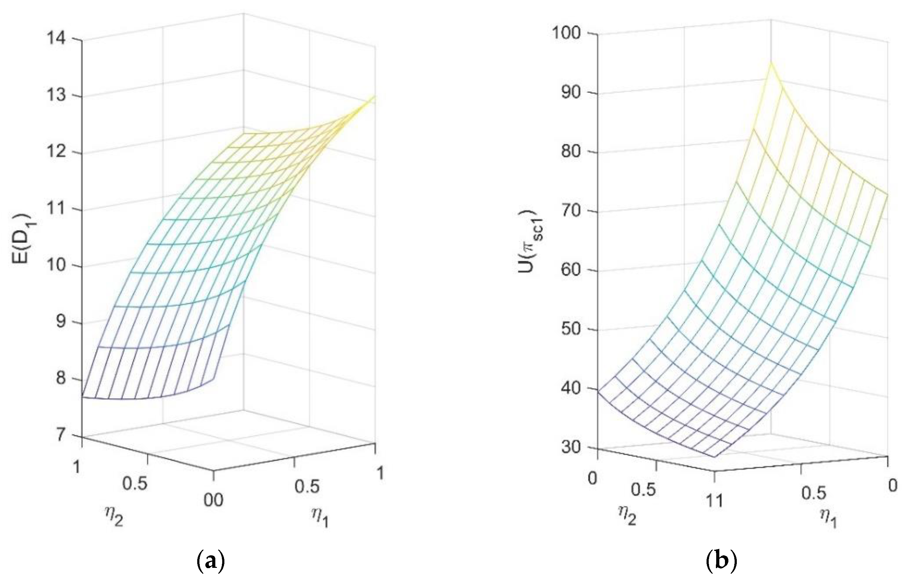
Figure 3.
Changes in the value of each variable with in the second case.
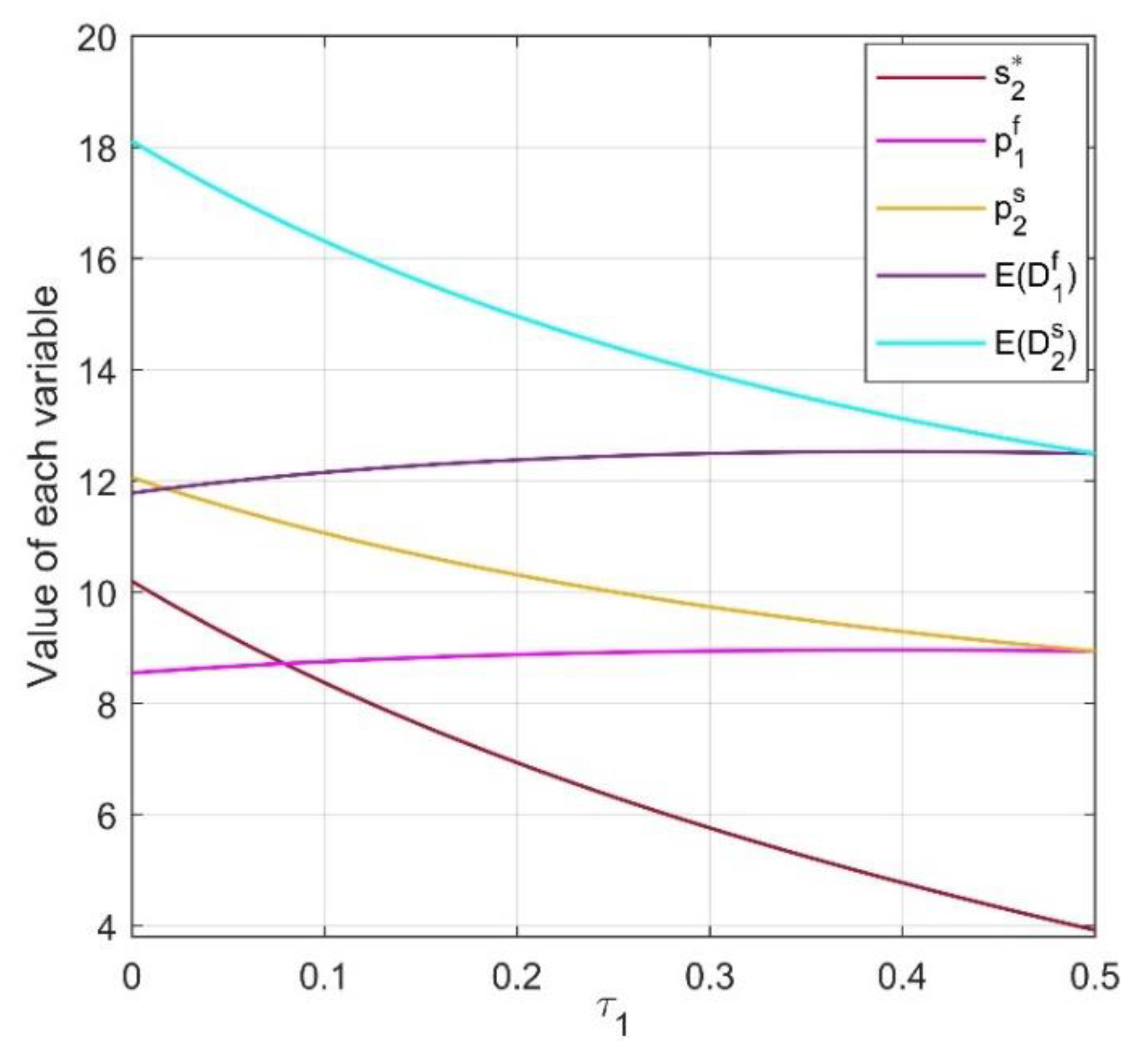
Figure 4.
Changes in total expected utility of the two supply chains with in the second case.

Figure 5.
Changes in the price with the free-riding coefficient in the fourth case.

Figure 6.
Changes in the total expected utility with the free-riding coefficient in the fourth case.
Figure 6.
Changes in the total expected utility with the free-riding coefficient in the fourth case.
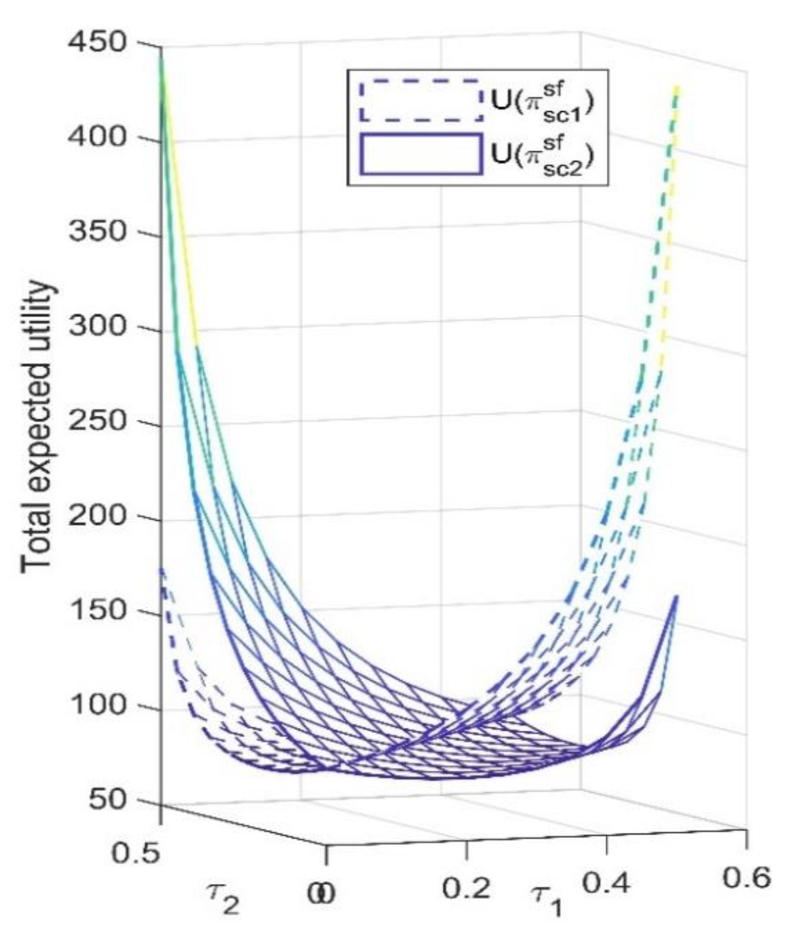
Figure 7.
Changes in effort level with free-riding coefficient in the fourth case.

Table 1.
Pricing varies with the degree of risk aversion.
| 0.2 | 0.2 | 10.24 | 10.24 | 12.03 | 14.88 | 14.88 | 12.03 | 22.08 | 22.08 |
| 0.5 | 9.95 | 8.30 | 11.04 | 10.68 | 14.24 | 9.59 | 19.39 | 13.65 | |
| 0.8 | 9.77 | 7.10 | 10.53 | 8.56 | 13.85 | 8.10 | 18.28 | 10.18 | |
| 0.5 | 0.2 | 8.30 | 9.95 | 9.59 | 14.24 | 10.68 | 11.04 | 13.65 | 19.39 |
| 0.5 | 8.09 | 8.09 | 8.88 | 10.31 | 10.31 | 8.88 | 12.28 | 12.28 | |
| 0.8 | 7.95 | 6.93 | 8.51 | 8.30 | 10.08 | 7.55 | 11.69 | 9.26 | |
| 0.8 | 0.2 | 7.10 | 9.27 | 8.10 | 13.85 | 8.56 | 10.53 | 10.18 | 18.28 |
| 0.5 | 6.93 | 7.95 | 7.55 | 10.08 | 8.30 | 8.51 | 9.26 | 11.69 | |
| 0.8 | 6.83 | 6.83 | 7.27 | 8.14 | 8.14 | 7.27 | 8.87 | 8.87 |
Table 2.
The total expected utility of each supply chain varies with the degree of risk aversion.
| 0.2 | 0.2 | 67.82 | 67.82 | 100.50 | 106.00 | 106.00 | 100.50 | 200.50 | 200.50 |
| 0.5 | 63.13 | 51.62 | 81.65 | 71.14 | 97.23 | 74.79 | 153.00 | 115.10 | |
| 0.8 | 60.30 | 41.67 | 72.85 | 53.52 | 92.04 | 59.56 | 135.30 | 80.46 | |
| 0.5 | 0.2 | 51.62 | 63.13 | 74.79 | 97.23 | 71.14 | 81.65 | 115.10 | 153.00 |
| 0.5 | 48.17 | 48.17 | 61.48 | 65.77 | 65.77 | 61.48 | 90.86 | 90.86 | |
| 0.8 | 46.08 | 38.94 | 55.16 | 49.69 | 62.57 | 49.30 | 81.43 | 64.34 | |
| 0.8 | 0.2 | 41.67 | 60.30 | 59.56 | 92.04 | 53.52 | 72.85 | 80.46 | 135.30 |
| 0.5 | 38.94 | 46.08 | 49.30 | 62.57 | 49.69 | 55.16 | 64.34 | 81.43 | |
| 0.8 | 37.29 | 37.29 | 44.39 | 47.39 | 47.39 | 44.39 | 57.97 | 57.97 |
Table 3.
Effort level changes with the degree of risk aversion.
| 0.2 | 0.2 | 10.93 | 10.93 | 20.13 | 20.13 |
| 0.5 | 7.34 | 10.25 | 17.29 | 11.07 | |
| 0.8 | 5.52 | 9.84 | 16.11 | 7.28 | |
| 0.5 | 0.2 | 10.25 | 7.34 | 11.07 | 17.29 |
| 0.5 | 6.93 | 6.93 | 9.64 | 9.64 | |
| 0.8 | 5.24 | 6.69 | 9.02 | 6.33 | |
| 0.8 | 0.2 | 9.84 | 5.52 | 7.28 | 16.11 |
| 0.5 | 6.69 | 5.24 | 6.33 | 9.02 | |
| 0.8 | 5.07 | 5.07 | 5.92 | 5.92 |
Table 4.
Pricing and total expected utility of the two supply chains in the second case.
| 0.2 | 0.2 | 11.96 | 11.96 | 90.40 | 73.24 | 11.44 | 10.70 | 89.20 | 71.66 |
| 0.5 | 11.15 | 9.26 | 75.60 | 42.93 | 10.84 | 8.57 | 78.16 | 53.81 | |
| 0.8 | 10.69 | 7.71 | 67.75 | 25.15 | 10.48 | 7.28 | 71.85 | 43.08 | |
| 0.5 | 0.2 | 9.51 | 11.47 | 56.32 | 66.87 | 9.11 | 10.31 | 65.62 | 66.05 |
| 0.5 | 8.94 | 8.94 | 46.73 | 39.03 | 8.69 | 8.30 | 58.11 | 49.85 | |
| 0.8 | 8.61 | 7.48 | 41.59 | 22.51 | 8.43 | 7.07 | 53.76 | 40.03 | |
| 0.8 | 0.2 | 8.03 | 11.18 | 35.69 | 63.12 | 7.70 | 10.08 | 51.91 | 62.74 |
| 0.5 | 7.59 | 8.75 | 28.91 | 36.73 | 7.38 | 8.14 | 46.26 | 47.49 | |
| 0.8 | 7.34 | 7.34 | 25.27 | 20.94 | 7.18 | 6.95 | 42.96 | 38.21 | |
Publisher’s Note: MDPI stays neutral with regard to jurisdictional claims in published maps and institutional affiliations. |
© 2022 by the authors. Licensee MDPI, Basel, Switzerland. This article is an open access article distributed under the terms and conditions of the Creative Commons Attribution (CC BY) license (https://creativecommons.org/licenses/by/4.0/).
Share and Cite
MDPI and ACS Style
Gao, T.; Wang, K.; Mei, Y.; He, S.; Wang, Y. Supply Chain Pricing Models Considering Risk Attitudes under Free-Riding Behavior. Mathematics 2022, 10, 1723. https://doi.org/10.3390/math10101723
AMA Style
Gao T, Wang K, Mei Y, He S, Wang Y. Supply Chain Pricing Models Considering Risk Attitudes under Free-Riding Behavior. Mathematics. 2022; 10(10):1723. https://doi.org/10.3390/math10101723
Chicago/Turabian StyleGao, Taiguang, Kui Wang, Yali Mei, Shan He, and Yanfang Wang. 2022. "Supply Chain Pricing Models Considering Risk Attitudes under Free-Riding Behavior" Mathematics 10, no. 10: 1723. https://doi.org/10.3390/math10101723
Note that from the first issue of 2016, this journal uses article numbers instead of page numbers. See further details here.