
Optimizing Costs in a Reliability System under Markovian Arrival of Failures and Reposition by K-Policy Inspection


1
Department of Statistics and Operational Research, University of Jaén, 23071 Jaén, Spain
2
Department of Statistics and Operational Research, University of Granada, 18071 Granada, Spain
*
Author to whom correspondence should be addressed.
Mathematics 2022, 10(11), 1918; https://doi.org/10.3390/math10111918
Submission received: 4 May 2022
/
Revised: 30 May 2022
/
Accepted: 31 May 2022
/
Published: 3 June 2022
(This article belongs to the Section Engineering Mathematics)
Abstract
:This paper presents an N warm standby system under shocks and inspections governed by Markovian arrival processes. The inspections detect the number of down units, and their replacement is carried out if there are a minimum K of failed units. This is a policy of the type used in inventory theory. The study is performed via the up and down periods of the system (cycle); the distribution of these random times and the expected costs for each period comprising the cycle are determined on the basis of individual costs due to maintenance actions (per inspection and replacement of every unit) and others due to operation or inactivity of the system, per time unit. Intermediate addressed calculus are the distributions of the number of inspections by cycle and the expected cost involving every inspection, depending on the number of replaced units. The system is studied in transient and stationary regimes, and some reliability measures of interest and the cost rate are calculated. An optimization of these quantities is performed in terms of the number K in a numerical example. This general model extends to many others in the literature, and, by using the matrix-analytic method, compact and algorithmic expressions are achieved, facilitating its potential application.
MSC:
90B251. Introduction
Systems with units in standby are common in industry. With units in reserve, the life of the machines enlarges. In reliability, this is a frequent structure. A warm standby is necessary in some cases in which access to the system is not immediate or difficult, as in meteorologic stations in remote locations. In these cases, an inspection allows for failed units to be detected and replaced. The alternative methods are to replace every unit when it fails or to replace all the units when they are nonoperational. In the first case, the number of replacements is greater than in the case we propose, and this increases the expected cost. In the second case, when the last operational unit fails, the system is nonoperational. This causes a stop in production until new units arrive. We propose an intermediate case in which the performance measures and the long-run cost rate can be optimized in terms of the number K.
Standby systems are common redundant structures, widely addressed in different domains. In reliability literature, they are often studied under several maintenance policies, repair modes, inspections and replacements. In [1], a redundant system performing phased missions exposed to random shocks was developed. Random inspections are considered in a redundant k-out-of-n: G system studied in [2], where potential loss of units is assumed, and [3] additionally incorporates multiple vacations on a cold standby system. Replacement policy K has been widely used as a useful tool to improve the availability of the system and the long-run cost rate. In [4,5], optimal repair–maintenance policies were applied to single systems. In the first one, repairable and nonrepairable failures are distinguished, the system is replaced at the Nth repairable failure or at the arrival of nonrepairable failures, whichever occurs first, and two replacement models were compared. In the second one, the system is periodically inspected every T units of time, and two types of preventive replacements are provided, deterministic after M inspections and opportunity-based after N minor failures. The optimal policy is formulated as a function of these parameters. The Markov process has been applied in the study of reliability systems due to its versatility and the analytic expressions of the main reliability measures. The limitation of these processes is that the staying times in states are exponentially distributed. A variety of shock and wear systems with different repair and replacement criteria have been studied in [6,7,8,9]. Authors in [10] considered preventive maintenance of items under a Poisson random shock process, with double effect. A stochastic network was constructed for studying a warm standby n-system with dissimilar components using a Markov process, and the structure of minimal paths was performed in [11,12]. In [13] this technique was used, considering inspections at random times defining a renewal process. In [14], an expression for the joint interval reliability was obtained using the Markovian methodology for a general system that can be applicable to standby systems. This measure is of interest in the power transmission line reliability. The replacement policy K was applied in [15], where a system with a limited number of repairs before a replacement is presented. Phase-type distributions and Markov renewal processes are used more and more in the literature due to their generality in applications and the versatility of the calculations. The following papers are related to these methods [16,17,18,19], among others. In [16], a repairable system under the influence of environment conditions was modeled, in which replacement policy K was performed so that after the -th failure, the system is not repaired but replaced. The renewal process due to the replacements of the system was studied. In addition, under this methodology, a warm standby system submitted to shocks was studied in [17]. The replacement of the system occurred when it was down, and the number of replacements of the system with time was determined. Other papers deal with standby systems with repair under multiple vacations. For instance, in [18], a repairable warm standby system undergoing shocks is addressed, where a repairman takes multiple vacations based on the N-policy. Phase-type distributions and MAPs play an important role in that model, and performance measures of interest are obtained for the system in transient and stationary regimes. Other related work is [19], concerning a cold standby repairable system which incorporates working vacations and vacation interruptions. The existing literature on reliability and maintenance modeling is extensive, and many works related to this one in some respect can be found under different methodologies, approaches and application domains. For instance, in [20], a model is proposed to determine the inspection and opportunistic maintenance strategies of floating offshore wind turbines. In [21], multiple failures and simultaneous replacements after inspection are considered in a complex system, while authors in [22] focused on the maintenance of the server system. In this case, a single server stands Markovian arrivals and random shocks. As mentioned before, replacement policy K has demonstrated to play an important role when availability system and cost-optimal decision problems are investigated, as discussed in [23,24]. These papers determined the number of preventive maintenance before the system replacement or the planned replacement time to minimize the expected cost rate, respectively. Meanwhile, authors in [15] pointed out the optimal number of corrective repairs prior to the reposition of the system; other studies of effectiveness are [25,26,27,28,29], and so on.
1.1. Contributions
We present a standby system with multiple components submitted for shocks affecting the online component and the standby one in a different ways and maintained by inspection and replacement using policy K. The procedure for studying these systems is based on the matrix-analytic methods (MAMs) that have proven to be useful in complex systems and that allow the results to be presented in a well-structured form. Moreover, the staying times in states are not necessarily exponentially distributed. This technique based on the state–space model seems to be appropriate for studying the reliability and maintenance of systems. In [30], different models are studied, discussed and compared. The arrival of the failures and inspections are governed by Markovian arrival processes (MAPs) that present two important properties: the interarrival times are not independent, and they extend many other arrival processes such as the Poisson process, the Markov-modulated Poisson process and the Phase-type renewal process. The replacement of the components occurs when an inspection arrives, and the number of down units reaches or surpasses a fixed number K. Extreme values in K, and are of frequent use in maintenance modeling. The dynamic of the system establishes consecutive operational and nonoperational periods, the cycles. Explicit expressions for the expected costs associated to the cycles are calculated by considering the random number of inspections in each period, the mean number of replaced units in every inspection and the expected length of the operational and nonoperational periods. For the system, the availability, the rate of failure and the mean number of replacements are obtained in a transient regime. A study of the optimization of the long-run cost rate and the availability in terms of the values of K and the mean time of inspections are performed in a numerical application.
This reliability system can also be applied to inventory control and risk analysis; failure, inspection, replacement and survival until time t can be substituted by demand, revision, shortage, reinstatement and no shortage until time t in inventory control and by claim, control of the number of claims, bankruptcy, and all claims until time t in risk analysis. In inventory control, this model is assimilated to a one; there is a total of N units to be sold, there is demand, and when the number in stock is less than K, an order is requested to the store to complete the stock to S units; in any other case, there is no order. This model is useful when the size of the stock is necessarily limited by the capacity of the available space, as is the case for cars and large machines. Under this policy, the costs of the transport of the units from the store to the shop can be cheaper if the requests include several units. The standby structure is appropriate for material degrading with time. The failures (demands), the inspections (revisions), and the replacements (requests) are random, and we consider probabilistic structures with dependence among the interarrival time of the occurrences.
The general hypotheses established for the proposed model and the compact expressions achieved by using the MAM methodology expand its application possibilities. Many particular models previously addressed in the literature can be derived from it.
1.2. Organization
The paper is organized as follows. The model is constructed in Section 2. In Section 3, the stationary distribution and some performance measures are calculated first. Second, the up and down periods in the cycles and the involved costs are carried out. Finally, the performance measures of the system are calculated in a transient regime. In Section 4, a numerical example illustrates the optimization model in terms of K, some reliability measures and the long-run cost rate.
2. The Model
Before describing the model, we give the definition of elements that play an important role in the application of the matrix-analytic method: the Kronecker operators, the Phase-type distributions and the Markovian arrival processes.
2.1. Definitions
Definition 1.
If A and B are rectangular matrices of orders respectively, their Kronecker product is the matrix of order , written in compact form as
The Kronecker sum of the square matrices C and D of orders p and q, respectively, is defined by where denotes the identity matrix of order k.
Definition 2.
The distribution function on of a phase-type distribution is
It is associated with a finite Markov process with one absorbent state. The initial vector of the process is . Matrix T is the submatrix of the generator of the process restricted to the transient states; it is nonsingular. Vector e is a column vector of 1’s. The absorption column vector is denoted by , and it satisfies The order of the matrix and vectors involved are the same. It is said that the distribution has representation , and it is written . is the distribution function of the first passage time of the Markov process for the absorbent state given the initial vector . The order of the distribution is the order of matrix T. A PH-renewal process is a renewal process whose distribution function is given by a PH-distribution.
Definition 3.
Let D be an irreducible infinitesimal generator of a Markov process. Let a sequence of matrices be non-negative and the matrix with non-negative off-diagonal entries. The diagonal entries of are strictly negative, and it is nonsingular. All the matrices are square and have the same order. It is assumed that
associated with this Markov process, there is a renewal Markov process performing an arrival process to real line operating as follows. Matrix governs the interarrival times, and matrix governs the arrival of type This is the MAP associated with the initial Markov process. The order of the MAP is the order of the involved matrices, and it is written .
2.2. Asumptions of the Model
Let a system be with N units. Initially one unit is online, and the other units are in warm standby. When the unit online fails, one of the units in standby, if any, becomes the online unit. Online and standby units are subject to shocks governed by two different and independent Markovian arrival processes. A shock cannot produce multiple failures to the standby units. The system is operational if at least one unit is up. The maintenance of the system is performed by inspection and replacement. The maintenance follows a K-policy: in every inspection, the number j of failed units is observed, . If the number of failed units is , all these units are replaced; in any other case, there is no action. Particular well-known cases are , in which all the failed units are replaced in every inspection, and , in which all the units have failed and are replaced. Once the units are replaced, they return to standby if there is one operating online. In any other case, one of the new units goes online. The costs associated with the maintenance are: : cost per inspection; : cost per replacement of every unit; : cost per unit of time that the system is nonoperational; : cost per unit of time that the system is operational and : cost for starting up the system after a failure. In advance, positive values in costs are interpreted as benefits, while negative values are interpreted as losses.
The assumptions of the system are the following:
- The online unit is submitted to shocks governed by the with initial vector c and order
- The standby units are submitted to shocks governed by the with initial vector d and order
- The inspections occur following the with initial vector h and order
- All the MAPs are independent.
2.3. Macro-States of the System
Macro-state i is the number of nonoperational units, . Three types of macro-states are distinguished: (1) , the online unit and at least one of the standby units are operational if they are determined by the phases of the MAPs in the assumptions 1, 2, 3, in this order, and the associated vector is , with , ; (2) the only operational unit is the online one, , the associated vector is , and (3) all the units are nonoperational; , the associated vector is .
To construct the generator, policy K allows for the grouping of the macro-states as follows: (1) , when an inspection occurs and the system occupies any of these macro-states, no unit is replaced; in the rest of the macro-states, there is replacement, and two types of macro-states are differentiated, (2) , and (3) , these are the border macro-states. The generator is constructed by blocks calculating the transition among these groups of macro-states.
2.3.1. Transition
Transition is governed by ; no shock arrives, and an inspection has no effect on the units. In Transition , if a failure occurs to one unit (online or standby), the phase of the inspection cannot change; it is governed by The rest of transitions and are identical, respectively, to and . No other transitions are possible.
Transitions from to any other macro-state are null, except that occurs when a shock arrives and it is governed by .
2.3.2. Transition
Transition is similar to , but now an inspection cannot occur; it is governed by . The same occurs for the rest of diagonal blocks . Transition is like , ; it is the same for , . Transition to occurs if there are two operational units, the online and the standby ones, and a shock arrives; then one of the two units fails: (a) if the online fails (governed by ), the MAP governing the arrival of shocks to the standby units can occupy any phase, and the standby unit becomes the online one; the inspection does not change (governed by I); and (b) similarly, the failure of the standby unit from any phase is governed by , the MAPs corresponding to the online unit and the inspection do not change. Taking into account the order of the macro-state vectors, the transition is governed by . Other upper transitions cannot occur since there are no multiple shocks.
2.3.3. Transition
Transition occurs when an inspection arrives (governed by ), and all the units are replaced. The MAPs related to the units do not change; it is governed by No other transitions are possible.
2.3.4. Transition
Transition occurs when an inspection arrives (governed by ), and the system reinitiates; it is governed by . Transition is governed by Transition is governed by since there is only one unit operating, and a failure occurs while the MAP governing the inspection does not change; the system fails. Transition occurs when an inspection arrives, and all the units are down; it is governed by . Transition is governed by . There are no more transitions.
The generator for is given by
For and we have, respectively,
with .
In Section 3, performance measures in a transient regime will be calculated in terms of the transition probability functions; these depend on generator Q.
3. Cycles of the System, Performance Measures and Costs
The system is first studied in a steady state. The stationary probability block vector is denoted by
The components are vectors associated with the macro-states. This is calculated from the equations , We assume that
Operating in these previous expressions, we have
with
The final expression for vector can be calculated from the following equations:
For , the equations and the solution are, respectively,
and for
with .
Once this distribution is obtained, the following performance measures are calculated.
The availability of the system is given by
The rate of occurrence of failures of the online unit is
The rate of occurrence of failures of the units in standby is
For the system, the rate of failure has the expression
3.1. Distribution of the Up and Down Periods
We carry out a study of the system via the up and down periods. The system is operational while occupying the macro-states , and it is down in macro-state N. The evolution of the system is an alternating sequence of up and down periods. A cycle is the time span of two consecutive up and down periods. The cycle initiates when the system occupies macro-state N, an inspection occurs (all the units are replaced) and the system reinitiates. From this point, the system is in the up period until all the units fail. Then it occupies a down period that finishes when a new inspection arrives. The cycles are of industrial interest; in some cases, the lifetime of the machines is expressed in terms of the completed cycles. The aging and the costs increase with the number of cycles. We consider the system with , in stationary regime. The other cases can be studied in a similar way. The up period of the system is denoted by ; it follows a -distribution. We calculate and . The system reinitiates from the macro-state 0 after an inspection, so . The occurrence of an inspection is governed by . Then, denotes the probability of the occurrence of an inspection and the probability of initiating the operational period given an inspection occurred. Vector is
Matrix is obtained from matrix Q suppressing the row and column of the nonoperational macro-state, N. The operational mean time is .
Let be the nonoperational period. It follows a -distribution with , derived from generator Q eliminating the rows and columns corresponding to the operational macro-states. The initial vector of this period is the probability of the occurrence of a failure of the system. This event occurs when the last operational unit fails, it is online. The initial macro-state for this event is following the vector , the failure is governed by , and then, it enters macro-state N. Then, the probability of occurrence of a down period is , since the MAPs affecting to shocks to the online and inspections do not change. Once it has occurred, the period initiates in any phase of macro-state N, then vector is
An alternative initial vector is . The mean time of the down period is . The time span of a cycle is , and follows a PH-distribution whose representation is well-known. The fraction of time that the system is up each cycle is given by
3.2. Costs by Cycles
The costs involved in the system are: by inspection (), by replacement (), by operational unit of time ( by nonoperational unit of time () and by the starting up of the system after a failure (). We centered on the costs involved in the cycles. The expected costs during an up and down period are denoted by and , respectively. The expected total cost per unit of time in a cycle is given by
The expected cost in a nonoperational period is
In advance, we also refer to as the long-run cost rate. Note that a positive value implies a benefit, while a negative value means a loss.
For calculating the expected cost during an operational period, we must know the number of inspections that occurred in this period and the expected cost of every inspection that depends on the number of replaced units. Let be the number of inspections during an operational period. We calculate the distribution of this random variable considering how the inspections arrive to the system during this period. The events that must have been taken into account are the following:
(a) There is neither inspection nor failure of the system;
(b) There is an inspection, and the system does not fail: the operational period continues;
(c) There is no inspection, and the system fails: the up period finishes.
Every event of these has an associated submatrix derived from generator Q collecting the transitions describing its occurrence. Given that the system is in an operational period, macro-state N is not included.
Matrix is associated with event (a):
Note that this matrix is obtained from Q eliminating the macro-state N, and replacing the blocks by , since inspections cannot occur in this event.
Matrix is associated with event (b):
This matrix includes the blocks associated with transitions involved in the occurrence of inspections without failure of the system. Therefore, blocks are eliminated since there is no failure; blocks are replaced by for (inspections without effect), maintained in column 0 and eliminated for because an inspection occurs.
Matrix is associated with event (c):
In this matrix, the transition blocks are collected, taking into account that there is no inspection, and the system fails.
From these matrices are calculated the probability of the occurrence of inspections, matrix F, and the probability of failure of the system, matrix , given by
These are, respectively, the matrices of the embedded Markov chain associated with the transitions due to inspections and failures of the system. The system fails from any phase, governed by . Note that transition is governed by so the last block of is ( is a column vector of order formed by the absorption rates to macro-state N for the different phases of the inspection. Given that there are only inspections and failures of the system, we have . Matrix F collects the probability of inspections and the probability of failures.
In macro-states , only inspections occur, and in macro-states , there are inspections and replacements. It is a partition of the set of operational macro-states. The costs associated with the macro-states are assigned in the following two matrices, where matrix denotes the identity matrix associated with macro-state :
The new diagonal block matrix summarizes the costs associated with the macro-states in which the inspections occur:
The up period initiates in macro-state 0 with initial probability vector The inspections occur in the macro-states with probabilities given by .
The expected cost due to the inspections and replacements during an up period in the different macro-states is given by matrix , and the total expected cost is
To clarify this result, we write matrices and in terms of the blocks of the partition of the set of macro-states; the arrival of an inspection without replacement occurs in the macro-states in u, and the ones including replacement after an inspection are in v. We can write
These blocks of matrix can be calculated by computational methods in practical cases. Note that and is a rectangular matrix with all the blocks null except the ones of the first column, as can be seen above.
We have, formally,
We interpret the block
The factors of the first summand indicate that the up period initiates in an element of u (really is 0), and an inspection occurs. The associated cost is given by , and after, the inspection returns to a macro-state in u. The second summand indicates that the up period initiates in an element of u, a failure occurs and there is a transition to v,. An inspection arrives later with associated cost given by and returns again to set u (really enters 0). The other block can be interpreted in a similar way.
Taking into account the initial conditions , the other block of the previous matrix is not used, and the mean cost per inspection in the up period is given by
Once the cost per inspection is calculated, we must calculate the number of inspections occurring in an up period, denoted by . Previously matrices F and have been defined. In terms of them, we have
This is the expression of a discrete -distribution with , being
The cost in the up period is denoted by , and the total mean cost in this period is
Taking into account the mean cost of the down period by cycle, the long-run cost rate is given by
3.3. Performance Measures
The system is studied in a stationary regime, but from matrix Q it is possible to calculate the transition probability matrix , with and macro-states, from the matrix equation under the initial condition . It is well-known that , and this expression is calculated using computational methods. The performance measures of the system in a transient regime can be deduced from this expression. Particularly, we calculate the availability , the failure rate of the system and the expected number of renewals of the system in the interval , denoted by . These measures will be determined later, along this section. The initial macro-state is assumed to be 0.
The reliability is the complementary of the distribution function of the first passage time of the Markov process Q for the absorbent state N. Eliminating the last row and column blocks in Q, and denoting this new matrix by , it is a PH-distribution given by
The availability has the expression
with and .
The failure rate of the system is
The mean number of replacements to the system in is calculated introducing new matrices derived from the ones of the MAPs and taking into account the arrivals of the event of interest. The transitions can be classified in two: those not producing a renewal of the system, governed by and those producing a renewal of the system, denoted by . The expressions of these matrices for , are
It can be seen that is a generator for any value of K.
The mean number of replacements in is
being the stationary vector associated with and .
The variance is
For and , the calculations are similar.
Some other measures can be calculated following the present procedure, including measures referred to the cycles defined before.
4. Numerical Example
A numerical and graphical study of the optimization of the maintenance (policy K) is applied to a system with . The unit time is denoted by u.t. The matrix parameters of the MAPs governing the arrival of shocks are
| Arrival of shocks to online unit | |||
| Arrival of shocks to the standby units | |||
| Occurrence of an inspection |
The assigned costs are
The study of this system comprises: (1) the performance reliability measures and the long-run cost rate, including values and graphics for the system with ; (2) a comparison of the measures for different values of K, tables and graphics; (3) a selection of the optimal policy given the performance measures and costs; and (4) an analysis of the frequency of the inspection in the measures for different values of K in the exponential case.
- Performance measures for
For , the values of the performance measures previously defined in a transient regime are given in Table 1.
The transient measures are plotted in Figure 1.
Figure 1 shows that the point is a singular point. The availability reaches the equilibrium at with a value close to . The failure rate of the system increases until and then decreases slowly. The number of replacements increases, as expected, and the rate seems to be linear.
In Table 2 the performance measures and costs by cycle are given.
The system is operational of the time of the cycle, the operational mean time by cycle is , and the mean time of the down period is . Therefore, the expected length of the cycle is . The long-run cost rate is .
- Comparing performance measures
In Figure 2, the availability of the system for all the values of K is plotted. The way in which the availability decreases with K is shown; the point in which all the curves approach to a constant is between and 1, nearer to 1. There is a significant difference between and the others.
In Figure 3 the failure rate of the system for all the values of K is plotted. Up to , the curves increases then, tends to be constant between 1 (exponential) and for , but for , the rate increases slowly and takes values greater than 3.
Figure 4 represents the mean number of replacements in the system for different values of K. As expected, all the plots increase with time and are approximately linear for for systems . The system has an expected number significantly different to the others.
In Table 3, the stationary distribution A, the mean operational time , the mean time of the cycle , the proportion of the operational time , and the long-run cost rate are given for all the values of K.
For an optimal policy K in terms of the operational time and costs, the values of and in terms of K are plotted in Figure 5. In both cases, the values decrease with K in a similar way.
- Availability and the long-run cost rate in terms of the inspection times
We consider the mean time of inspections a parameter and determine the performance measures in terms of it. This is a quantity that can be established by the researcher, and it allows us to optimize some performance measures. It is assumed that the inspection times are exponentially distributed. In Figure 6, the long-run cost rates in terms of the different values of are given for the inspection mean time (IMT) . For , the benefits increase when the mean time between inspections increases. For , the behavior is different. For , the long-run cost rates for and are identical and less than for . For , the optimal long-run cost rate is reached for . Until this value, the long-run cost rate is notably increasing; then it decreases shortly for .
In Figure 7, the long-run cost rates in terms of the mean time of inspections for different values of K are plotted. It is observed that the behavior of the graphics are very similar. It is optimum when the mean time between inspections is and
In Figure 8, the availability is plotted in terms of the mean time between inspections for different values of For , the availability is less than in the other cases, and for it reaches the greatest value. The availability decreases in all cases with the mean time between inspections increasing; the decreasing is affected by the number of units.
5. Conclusions
A major novelty in the present paper is the inclusion of the MAMs for the study of complex systems. The generality of the assumptions extends the application of the model to other systems. We can see that by handling the matrix calculations, it is possible to express quantities algorithmically since the operations in the formulae involving matrices are presented in a well-structured form. This is highlighted in the study of the costs and in the calculation of the performance measures. These measures have been calculated for the cycles and for the total system, since the aging of a system can be measured by the time or by the number of cycles. Applying the methods to the study of a system and varying the parameters depending on the researcher reveals that complete information onthe quantities affecting the performance of the system can be obtained. By adding new assumptions to the system, such as lifetime of the units, repairs and others, the study can be extended to more complex systems. Moreover, this methodology is suitable for the extension of the model in other ways. For instance, considering an appropriate MAP, simultaneous failures in units can be incorporated, and a natural continuation takes place when units in the system are K-grouped, following a modular structure. Many industrial systems have this structure; it can allow time and cost reductions when analysis of failures and maintenance, such as replacements, are set by blocks.
Author Contributions
Formal analysis, D.M.-C. and R.P.-O.; Investigation, R.P.-O.; Methodology, D.M.-C. and R.P.-O.; Software, D.M.-C.; Supervision, R.P.-O.; Writing—original draft, D.M.-C.; Writing—review & editing, R.P.-O. All authors have read and agreed to the published version of the manuscript.
Funding
This research received no external funding.
Data Availability Statement
Not applicable.
Conflicts of Interest
The authors declare no conflict of interest.
Abbreviations
| shock arrival process for online unit | |
| shock arrival process for standby units | |
| inspection arrival process | |
| identity matrix of order r | |
| column vector of 1’s of order r | |
| generator of the process under policy K | |
| steady state vector associated with the macro-state i | |
| steady state vector | |
| A | steady state availability |
| rate of occurrence of failures for online unit | |
| rate of occurrence of failures for standby units | |
| v | rate of occurrence of failures for the system |
| distribution of the up period of the system, | |
| distribution of the down period of the system, | |
| length of a cycle of the system | |
| expected length of the up period of the system | |
| expected length of the down period of the system | |
| expected length of a cycle of the system | |
| cost per inspection | |
| cost per every unit replacement | |
| cost by operational unit time | |
| cost by nonoperational unit time | |
| cost due to the starting-up of the system | |
| expected cost during an up period | |
| expected cost during a down period | |
| expected cost per inspection, depending on the number of replacements, | |
| in the up period | |
| expected number of inspections in the up period | |
| long-run cost rate | |
| availability of the system in time t | |
| reliability of the system in time t | |
| mean number of replacements of the system | |
| failure rate of the system in time t |
References
- Levitin, G.; Finkelstein, M.; Dai, Y. Redundancy optimization for series-parallel phased mission systems exposed to random shocks. Reliab. Eng. Syst. Saf. 2017, 167, 554–560. [Google Scholar] [CrossRef]
- Ruiz-Castro, J.E. A complex multi-state k-out-of-n: G system with preventive maintenance and loss of units. Reliab. Eng. Syst. Saf. 2020, 197, 106797. [Google Scholar] [CrossRef]
- Ruiz-Castro, J.E. Optimizing a Multi-State Cold-Standby System with Multiple Vacations in the Repair and Loss of Units. Mathematics 2021, 9, 913. [Google Scholar] [CrossRef]
- Wang, G.J.; Zhang, Y.L. Optimal repair-replacement policies for a system with two types of failures. Eur. J. Oper. Res 2013, 226, 500–506. [Google Scholar] [CrossRef]
- Badía, F.G.; Berrada, M.D.; Lee, H. An study of cost effective maintenance policies: Age replacement versus replacement after N minimal repairs. Reliab. Eng. Syst. Saf. 2020, 201, 106949. [Google Scholar] [CrossRef]
- Zhang, Y.L.; Wang, G.J. A deteriorating cold standby repairable system with priority in use. Eur. J. Oper. Res 2007, 183, 278–295. [Google Scholar] [CrossRef]
- Zhang, Y.L.; Wang, G.J. A geometric process repair model for a repairable cold standby system with priority in use and repair. Reliab. Eng. Syst. Saf. 2009, 94, 1782–1787. [Google Scholar] [CrossRef]
- Leung, K.N.F.; Zhang, Y.L.; Lai, K.K. Analysis for a two-dissimilar-component cold standby repairable system with repair priority. Reliab. Eng. Syst. Saf. 2011, 96, 1542–1551. [Google Scholar] [CrossRef]
- Yuang, I.; Meng, S.-Y. Reliability analysis of a warm standby repairable system with priority in use. Appl. Math. Model. 2011, 35, 4295–4303. [Google Scholar] [CrossRef]
- Cha, J.H.; Finkelstein, M.; Levitin, G. On preventive maintenance of systems with lifetimes dependent on a random shock process. Reliab. Eng. Syst. Saf. 2017, 168, 90–97. [Google Scholar] [CrossRef]
- Azaron, A.; Katagiri, H.; Sakawa, M.; Modarres, M. Reliability function of a class of time-dependent systems with standby redundancy. Eur. J. Oper. Res 2005, 64, 376–386. [Google Scholar] [CrossRef]
- Azaron, A.; Katagiri, H.; Kato, K.; Sakawa, M. Reliability evaluation of multi-component cold-standby redundant systems. Appl. Math. Comput. 2006, 173, 137–149. [Google Scholar] [CrossRef]
- Dieulle, L. Reliability of several component sets with inspections at random times. Eur. J. Oper. Res. 2002, 139, 96–114. [Google Scholar] [CrossRef]
- Csenki, A. On the three-state weather model of transmission line failures. Proc. Inst. Mech. Eng. O J. Risk Reliab. 2007, 139, 217–228. [Google Scholar] [CrossRef]
- Montoro-Cazorla, D.; Pérez-Ocón, R. Shock and wear degradating systems under three types of repair. Appl. Math. Comput. 2012, 218, 11727–11737. [Google Scholar] [CrossRef]
- Montoro-Cazorla, D.; Pérez-Ocón, R. A shock and wear system under environmental conditions subject to internal failures, repair and replacement three types of repair. Reliab. Eng. Syst. Saf. 2012, 99, 55–61. [Google Scholar] [CrossRef]
- Montoro-Cazorla, D.; Pérez-Ocón, R. A warmstandby system under shocks and repair governed by a MAPs. Reliab. Eng. Syst. Saf. 2016, 152, 331–338. [Google Scholar] [CrossRef]
- Baolian, L.; Cui, L.; Wen, Y.; Shen, J. A cold standby repairable system with working vacations and vacation interruption following Markovian arrival process. Reliab. Eng. Syst. Saf. 2015, 142, 1–8. [Google Scholar]
- Baolian, L.; Wen, Y.; Kang, S.; Qiu, Q. A multiple warm standby repairable system under N-policy with multiple vacations following Markovian arrival process. Commun. Stat.-Theory Methods 2020, 49, 3609–3634. [Google Scholar]
- Li, H.; Huang, C.G.; Guedes Soares, C. A Real-Time Inspection and Opportunistic Maintenance Strategies for Floating Offshore Wind Turbines. Ocean Eng. 2022, 256, 111433. [Google Scholar] [CrossRef]
- Montoro-Cazorla, D.; Pérez-Ocón, R. Constructing a Markov process for modelling a reliability system under multiple failures and replacements. Reliab. Eng. Syst. Saf. 2018, 173, 34–47. [Google Scholar] [CrossRef]
- Chakravarthy, S.R. Maintenance of a deteriorating single system with Markovian arrivals and random shocks. Eur. J. Oper. Res. 2012, 222, 508–522. [Google Scholar] [CrossRef]
- Castro, I.T. A model imperfect preventive maintenance with dependent failure modes. Eur. J. Oper. Res. 2009, 196, 217–224. [Google Scholar] [CrossRef]
- Castro, I.T.; Barros, A.; Grall, A. Age-based preventive maintenance for passive components submitted to stress corrosion cracking. Math. Comput. Model. 2011, 54, 598–609. [Google Scholar] [CrossRef]
- Huynh, K.T.; Barros, A.; Bérenguer, C.; Castro, I.T. A periodic inspection and replacement policy for systems subject to competing failure modes due to degradation and traumatic events. Reliab. Eng. Syst. Saf. 2011, 96, 497–508. [Google Scholar] [CrossRef] [Green Version]
- Wang, J.; Qiu, Q.; Wang, H. Joint optimization of condition-based and age-based replacement policy and inventory policy for a two-unit series system. Reliab. Eng. Syst. Saf. 2021, 205, 107251. [Google Scholar] [CrossRef]
- Ouaret, S.; Kennéa, J.P.; Gharbi, A. Production and replacement policies for a deteriorating manufacturing system under random demand and quality. Eur. J. Oper. Res. 2018, 264, 623–636. [Google Scholar] [CrossRef]
- Zhai, Q.; Peng, R.; Xing, L.; Yang, J. Reliability of demand-based warm standby systems subject to fault level coverage. Appl. Stoch. Model. Bus. Ind. 2015, 31, 380–393. [Google Scholar] [CrossRef]
- Liu, X.; Yang, T.; Pei, J.; Liao, H.; Pohl, E.A. Replacement and inventory control for a multi-customer product service system with decreasing replacement costs. Eur. J. Oper. Res. 2019, 273, 561–574. [Google Scholar] [CrossRef]
- Distefano, S.; Longo, F.; Trivedi, K.S. Investigating dynamic reliability and availability through state-space models. Comput. Math. Appl. 2012, 64, 3701–3716. [Google Scholar] [CrossRef] [Green Version]
- Bellman, R. Introduction to Matrix Analysis; McGraw-Hill: New York, NY, USA, 1970. [Google Scholar]
- Neuts, M.F. Matrix-Geometric Solutions in Stochastic Models—An Algorithm Approach; John Hopkins, University Press: Baltimore, MD, USA, 1981. [Google Scholar]
Figure 1.
Plot of for .
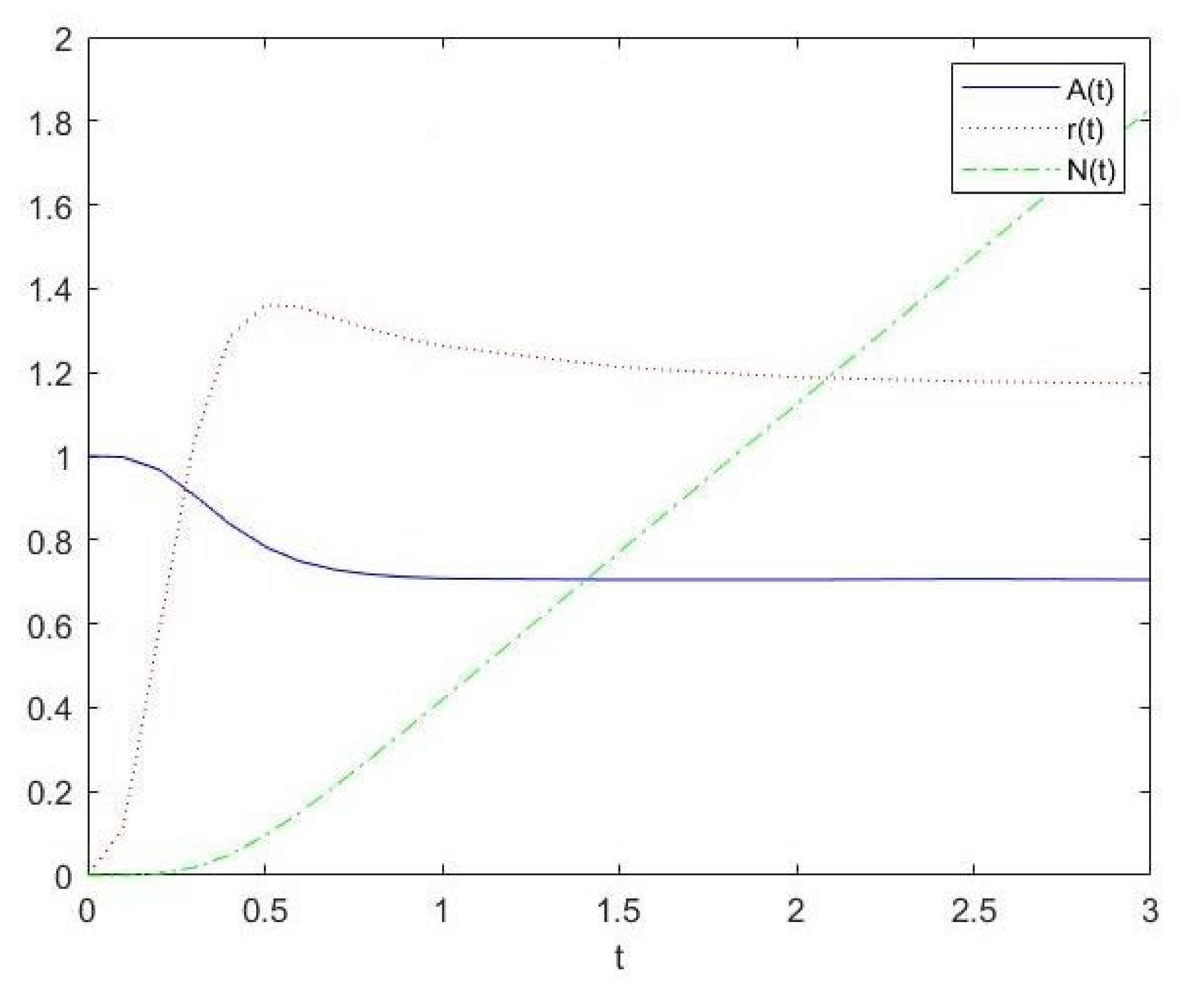
Figure 2.
Availability function for systems .
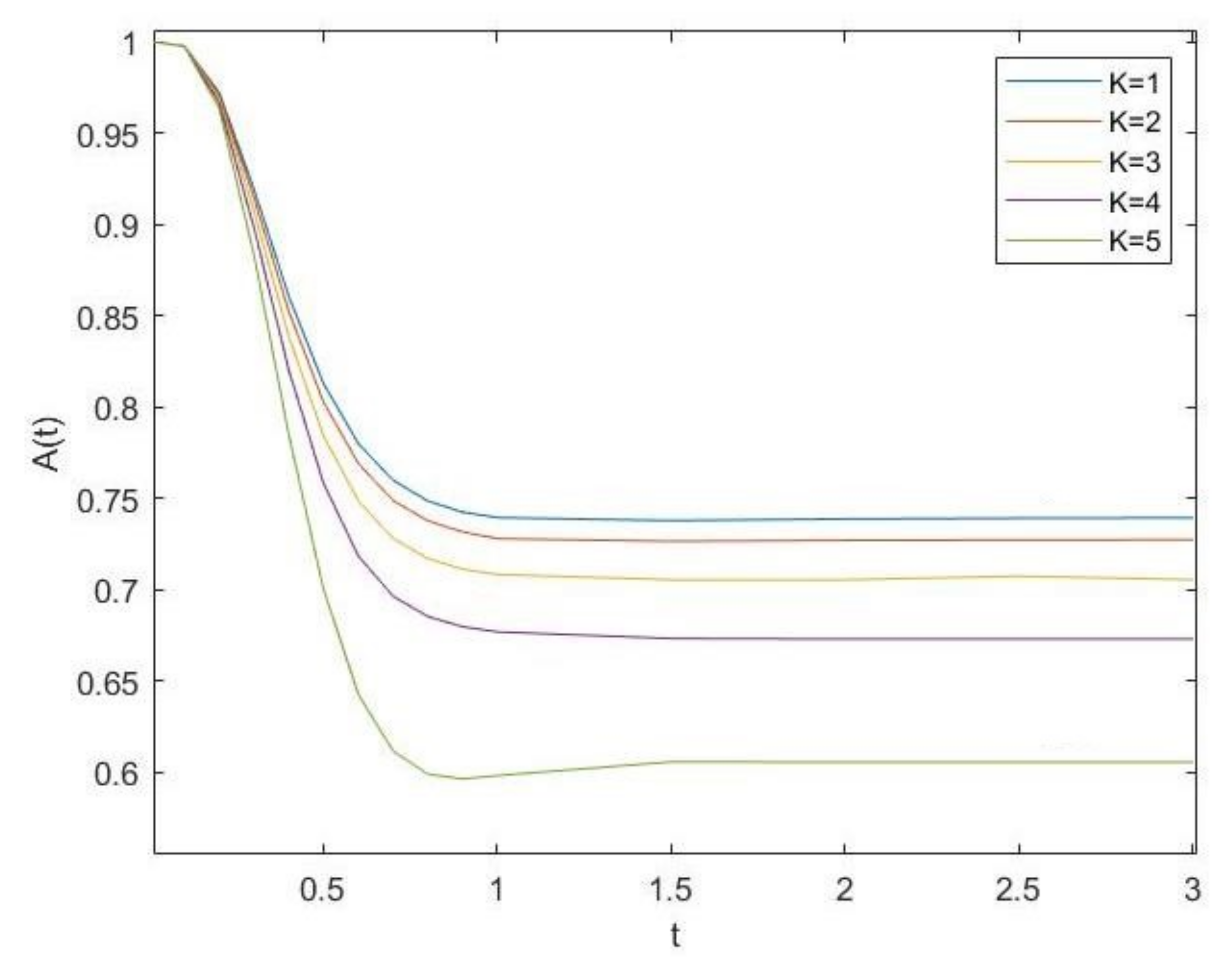
Figure 3.
Rate of system failure function for systems .
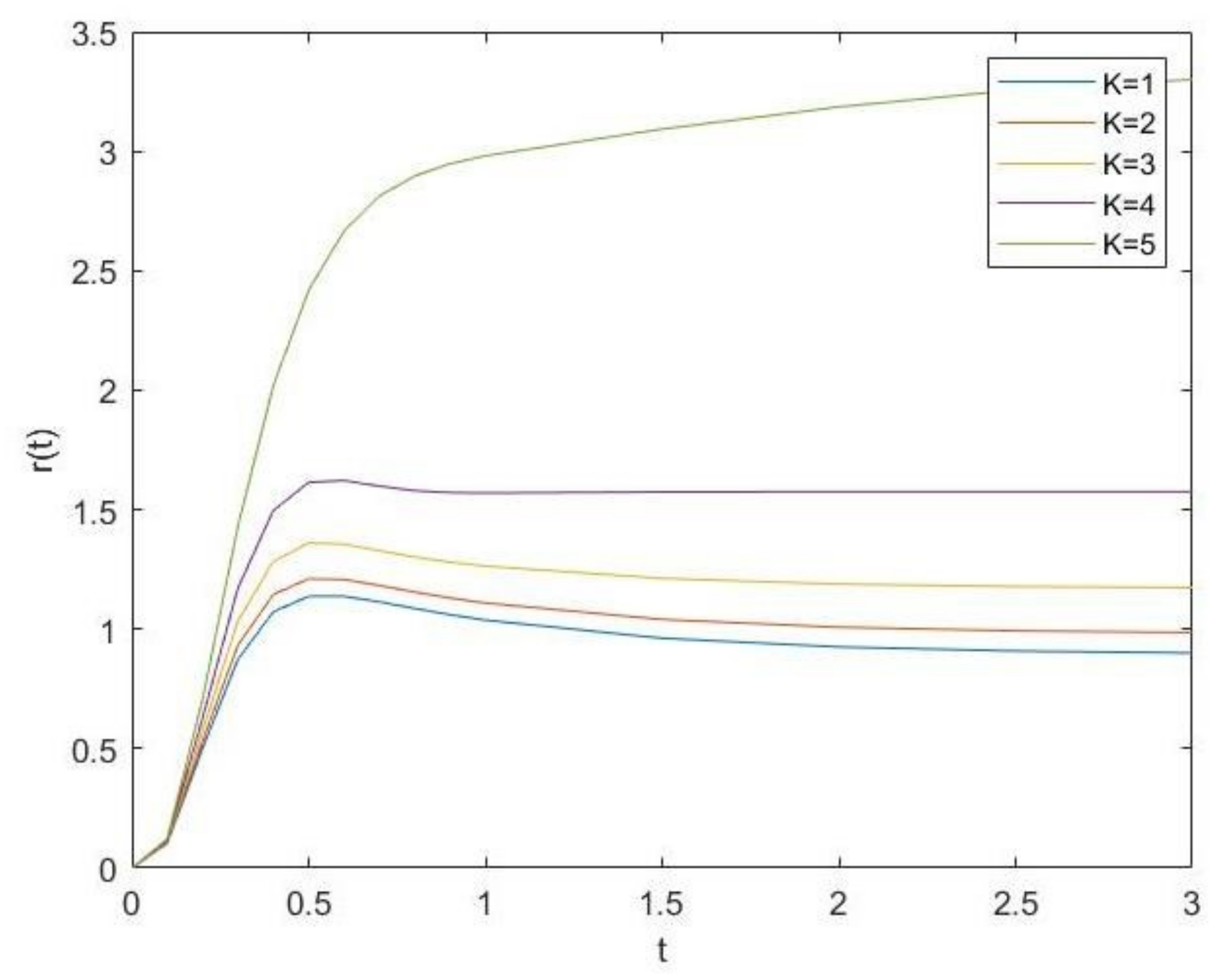
Figure 4.
Mean number of replacements for systems .
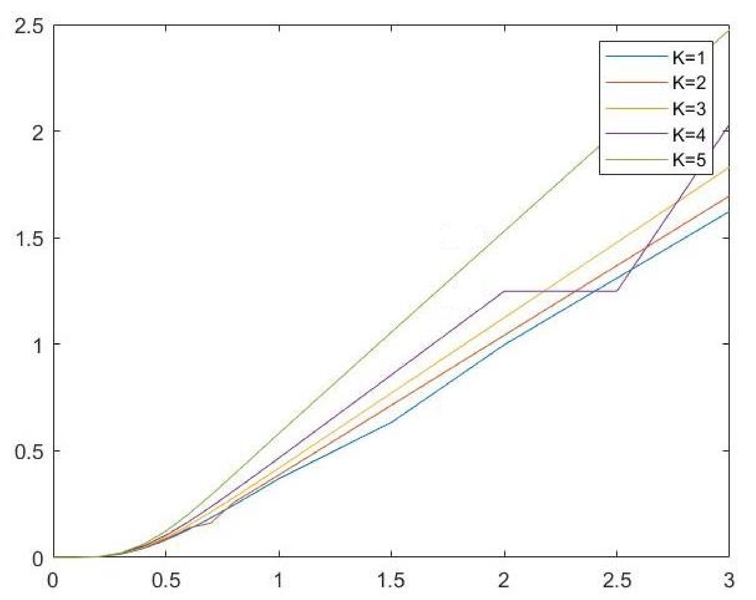
Figure 5.
Fraction of operational time by cycle and the long-run cost rate versus K.
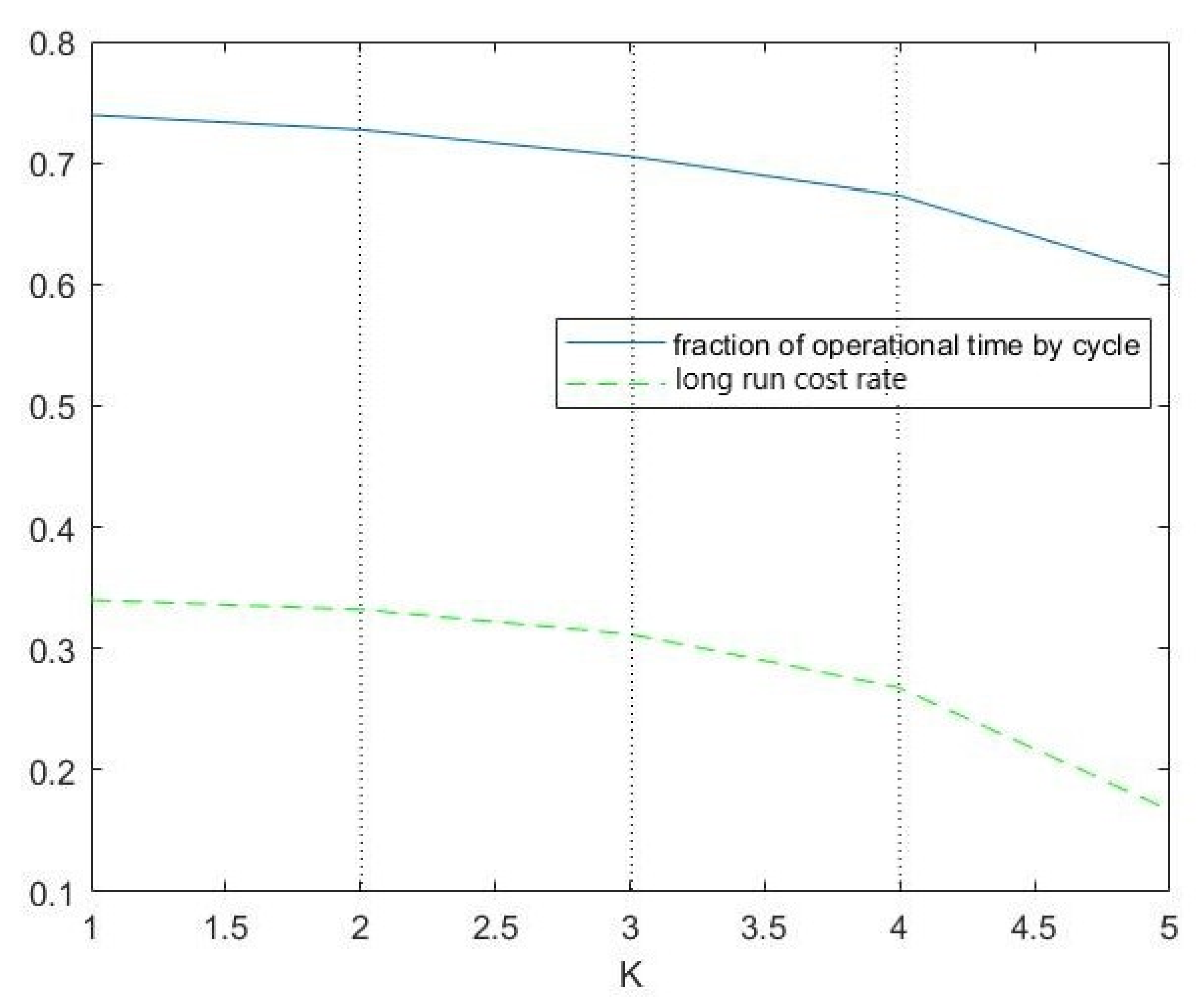
Figure 6.
The long-run cost rate versus K for .
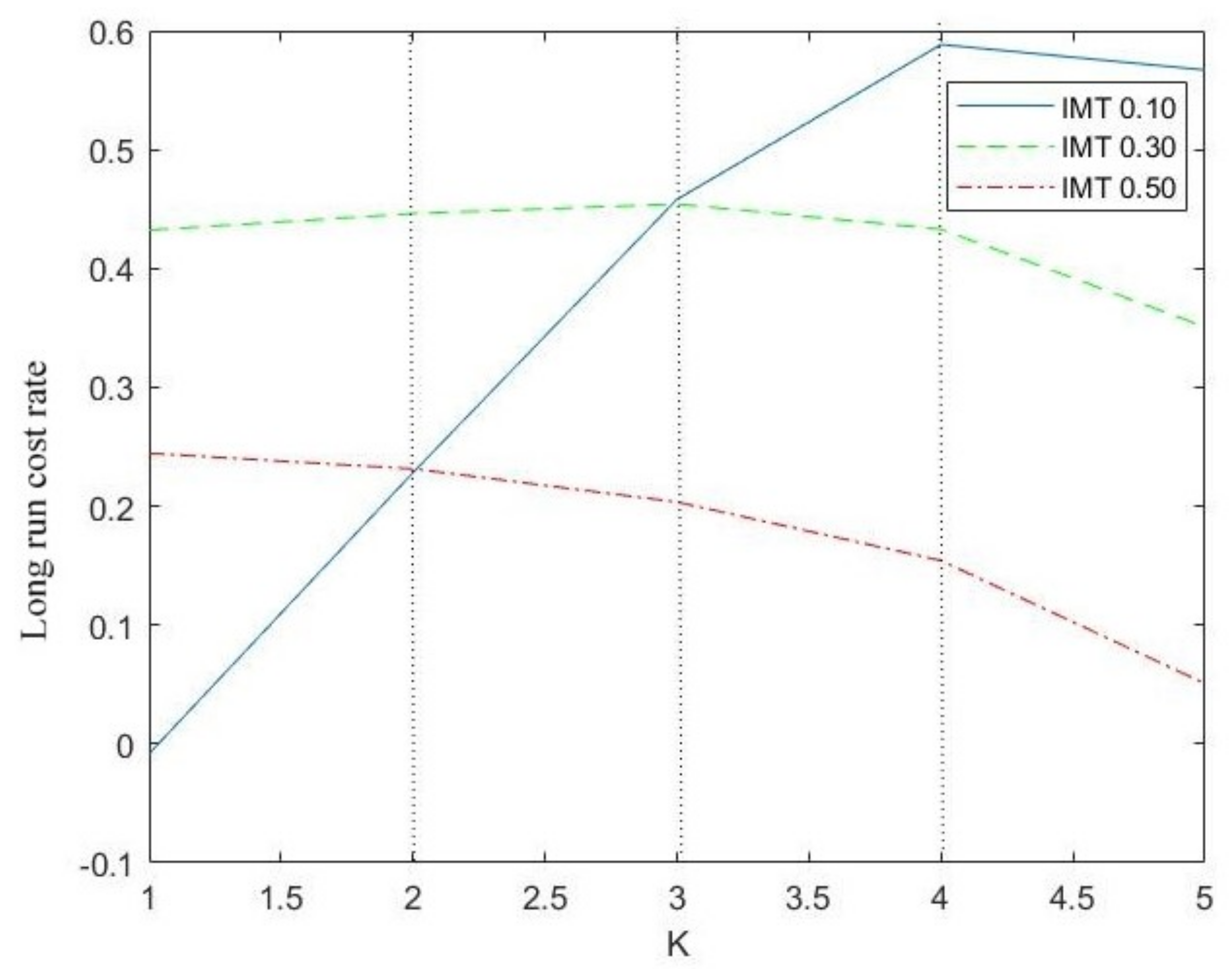
Figure 7.
The long-run cost rate in terms of for different values of K.
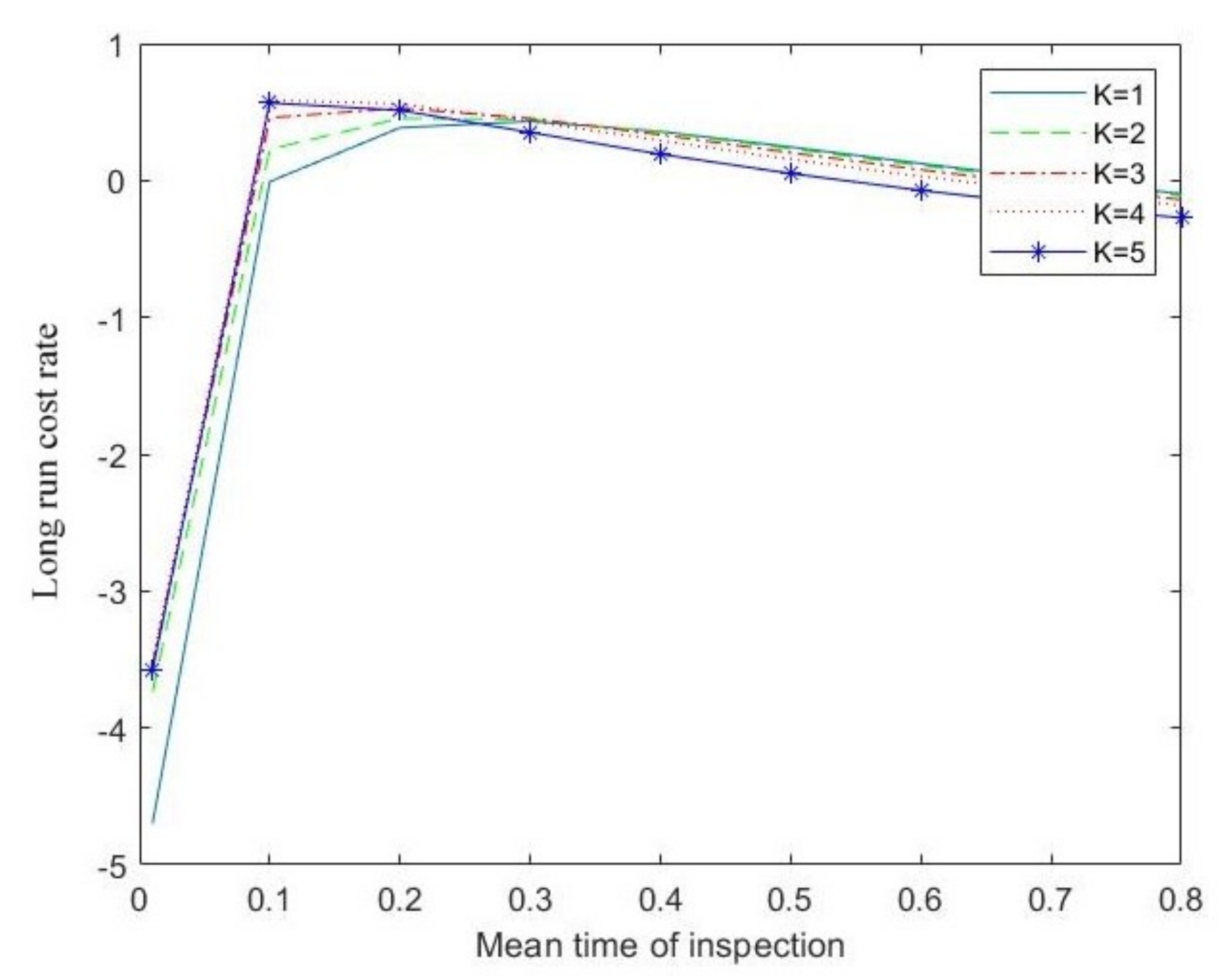
Figure 8.
Availability in terms of the mean time between inspections for different values of K.


Table 1.
Performance measures in transient regime for .
| t | 0 | 1 | |||||||||
|---|---|---|---|---|---|---|---|---|---|---|---|
| 1 | |||||||||||
| 0 | |||||||||||
| 0 | 0 |
Table 2.
Peformance measures and costs by cycle for .
| Policy | A | CT | |||
|---|---|---|---|---|---|
Table 3.
Performance measure and the long-run cost rate for systems .
| Policy | A | ||||
|---|---|---|---|---|---|
Publisher’s Note: MDPI stays neutral with regard to jurisdictional claims in published maps and institutional affiliations. |
© 2022 by the authors. Licensee MDPI, Basel, Switzerland. This article is an open access article distributed under the terms and conditions of the Creative Commons Attribution (CC BY) license (https://creativecommons.org/licenses/by/4.0/).
Share and Cite
MDPI and ACS Style
Montoro-Cazorla, D.; Pérez-Ocón, R. Optimizing Costs in a Reliability System under Markovian Arrival of Failures and Reposition by K-Policy Inspection. Mathematics 2022, 10, 1918. https://doi.org/10.3390/math10111918
AMA Style
Montoro-Cazorla D, Pérez-Ocón R. Optimizing Costs in a Reliability System under Markovian Arrival of Failures and Reposition by K-Policy Inspection. Mathematics. 2022; 10(11):1918. https://doi.org/10.3390/math10111918
Chicago/Turabian StyleMontoro-Cazorla, Delia, and Rafael Pérez-Ocón. 2022. "Optimizing Costs in a Reliability System under Markovian Arrival of Failures and Reposition by K-Policy Inspection" Mathematics 10, no. 11: 1918. https://doi.org/10.3390/math10111918
Note that from the first issue of 2016, this journal uses article numbers instead of page numbers. See further details here.