
Lie Symmetries of the Nonlinear Fokker-Planck Equation Based on Weighted Kaniadakis Entropy
by
 , , and
Iulia-Elena Hirica
1 ,
,
Cristina-Liliana Pripoae
2,
Gabriel-Teodor Pripoae
1 and
Vasile Preda
1,3,4,* 1
Faculty of Mathematics and Computer Science, University of Bucharest, Academiei 14, RO-010014 Bucharest, Romania
2
Department of Applied Mathematics, The Bucharest University of Economic Studies, Piata Romana 6, RO-010374 Bucharest, Romania
3
“Gheorghe Mihoc-Caius Iacob” Institute of Mathematical Statistics and Applied Mathematics of Romanian Academy, 2. Calea 13 Septembrie, Nr. 13, Sect. 5, RO-050711 Bucharest, Romania
4
“Costin C. Kiritescu” National Institute of Economic Research of Romanian Academy, 3. Calea 13 Septembrie, Nr. 13, Sect. 5, RO-050711 Bucharest, Romania
*
Author to whom correspondence should be addressed.
Mathematics 2022, 10(15), 2776; https://doi.org/10.3390/math10152776
Submission received: 25 July 2022
/
Revised: 1 August 2022
/
Accepted: 2 August 2022
/
Published: 4 August 2022
(This article belongs to the Special Issue Probability, Statistics and Their Applications 2021)
Abstract
:The paper studies the Lie symmetries of the nonlinear Fokker-Planck equation in one dimension, which are associated to the weighted Kaniadakis entropy. In particular, the Lie symmetries of the nonlinear diffusive equation, associated to the weighted Kaniadakis entropy, are found. The MaxEnt problem associated to the weighted Kaniadakis entropy is given a complete solution, together with the thermodynamic relations which extend the known ones from the non-weighted case. Several different, but related, arguments point out a subtle dichotomous behavior of the Kaniadakis constant k, distinguishing between the cases and . By comparison, the Lie symmetries of the NFPEs based on Tsallis q-entropies point out six “exceptional” cases, for: , , , , and .
Keywords:
nonlinear Fokker-Planck equation; nonlinear diffusive equation; Lie symmetries; weighted entropy; MaxEnt problem; Kaniadakis entropy; Tsallis entropy; STM entropy; Bregman divergence; partial differential equationsMSC:
35Q84; 22E70; 35Q82; 70G65; 82C31; 94A17; 53B121. Introduction
The nonlinear Fokker-Planck equation (NFPE) is an important parabolic partial differential equation (PDE), which is perhaps better known through some of its particular cases: the heat equation and the nonlinear diffusion equation. Its roots and main applications are in Statistical Mechanics, but many other domains benefit from its versatility to model various phenomena, where a probability density function (PDF) of the velocity of a particle evolves in time under the action of both deterministic and random fields of force. More general details may be found in the monographs [1,2,3,4] and especially, in [5]. A list of recent research papers concerning various applications of the NFPE includes, e.g., [6,7,8,9,10,11,12,13,14,15,16].
When exact general solutions of a PDE are not available, as is the case of the NFPE too, one may look for indirect/qualitative information about them. A powerful method is the search for symmetries. The Lie symmetries of the NFPE are prolongations of vector fields on an open set of and they span a Lie algebra, which provides geometric information about the solutions of the NFPE and is invariant with respect to some specific group action. The monograph of Olver [17] and the surveys [18,19], for example, offer a clear panorama of the vast field of Lie symmetries in general. Early contributions to the study of the Lie symmetries associated to the linear FPE and the NFPE, related to our paper, may be found in [20,21,22,23].
We point out, as a particular fundamental case, the NFPEs based on some entropy functional, which model remarkable physical phenomenons in Statistical Mechanics. The following papers are related to the NFPE associated to the Tsallis, Kaniadakis, Sharma–Taneja–Mittal entropies [24,25,26] with references therein (see also the surveys [27,28]). In our paper [29], we studied the Lie symmetries of an NFPE, based on a weighted Tsallis entropy, as a generalization of the setting in [24]. This extension, from the non-weighted to the weighted entropy, is motivated by the importance of integrating the quantitative, objective and probabilistic concept of information with the qualitative, subjective and non-stochastic concept of utility (see [30,31] and the more recent [27,32,33,34,35,36,37,38]).
Given a specific distribution of probability, an important optimization problem is to maximize a given entropy functional, which is subject to some a priori constraints [39,40]. For many families of entropy functionals, this MaxEnt problem received (by a standard method) a specific solution (e.g., [26,41,42,43,44]).
The interested reader may find, in our recent paper [29], a short historical review and references about the emergence of the notions of NFPE, Lie symmetries, weighted entropy and MaxEnt optimization problems.
1.1. The Content of the Paper
In Section 2, we fix the notations and the conventions concerning the NFPE and its Lie symmetries, closely following [17,24,45].
In Section 3, we recall some examples of remarkable entropies (Tsallis, Kaniadakis) and the procedure of weighting a given entropy functional. For a fixed PDF, a fixed potential energy function and a fixed entropy functional, we remind the associated notions of the energy average function, of the Lyapunov functional and of the current density.
The next three sections contain the main results of the paper. In Section 4, we calculate the variation of the Lyapunov function based on a weighted Kaniadakis entropy. Starting with its associated current density, we determine the corresponding NFPE. A formula linking the drift function , the diffusion function and the so-called “drift” constant D is established. We prove that the Lyapunov functional is non-increasing in time, and we interpret the Bregman divergence as a “distance” function, which is measured through Lyapunov values differences.
In Section 5, we use the Theorem 3 from our paper [29] in order to determine the Lie symmetries of the NFPE associated to a weighted Kaniadakis entropy. We detail the case of the classical (non-weighted) Kaniadakis entropy, and we point out a remarkable behavior of the constant k: the cases and lead to completely different symmetry patterns. We consider also an important particular case (the nonlinear diffusive equation) and we recover, apart from its Lie symmetries enunciated in [45], a genuine new family of symmetries, which fit into the classification from [25]. For all these old and new Lie symmetries, we characterize the spanned Lie (sub)algebras.
In Section 6, we solve the MaxEnt problem associated to the weighted Kaniadakis entropy, and we compare it to the non-weighted case. In this context, some new “weighted” generalizations of the thermodynamic relations are also proven. The dichotomous behavior of the Kaniadakis constant k is again highlighted in connection with the solvability of the MaxEnt problem.
Section 7 provides a detailed comparison of the Lie symmetries from Section 5, those in our paper [29] concerning the NFPE based on the weighted Tsallis entropy and the interesting classification of Sinkala, for the NFPE based on the Sharma–Taneja–Mittal (STM) entropy [25]. We point out two cases: with or without momentum convergence restrictions for the STM entropies. Unexpectedly, six “exceptional” values of the Tsallis entropy constant q emerge: , , , , and . We quote several papers where these values (or close ones) arose, both theoretically and empirically, in various applications of the Tsallis entropy. It seems that these values act as “singular” points in the “space of Tsallis entropies” and are able to signal the stochastic phenomena whose apparent “stability” is determined by a hidden (maximal) “symmetry”. As this topic is beyond the mainstream idea of the paper, we included it in Appendix A with some challenging speculations.
1.2. Conventions
In the sequel, the integrals are always supposed to be correctly defined and to commute with the partial derivatives. All the functions are supposed differentiable (“smooth”), even if, eventually, a weaker assumption would be sufficient (as continuity or integrability).
2. Nonlinear Fokker-Planck Equations in One Dimension
Denote by U an open subset of and let be a time-dependent probability density function (PDF) defined on . Consider a drift and a (non-negative) diffusion coefficient defined on . By definition, , . The associated NFPE in one (spatial) dimension is defined by the formula
written also as
where
is the nonlinear Fokker-Planck operator and I is the identity operator, i.e., .
Denote as the current function, which is defined by
Then, (1) and (2) are equivalent with
which is called the continuity equation.
In particular, for and , we obtain the linear Fokker-Planck equation (LFPE)
We fix now an NFPE (2), and we consider a family of linear differential operators of the form [17]
with (differentiable) coefficients , and defined on . We call L a Lie symmetry operator for (or for the NFPE (2)) if there exists a (differentiable) function on , satisfying the condition
A Lie symmetry operator L for maps solutions of (2) into solutions of (2). The set of all these operators forms a (possible infinite dimensional) Lie algebra, containing significant information about the symmetries of the solutions of the NFPE.
For the LFPE, the corresponding Lie symmetries were determined in [20,21,22]. The papers [24,45] present the Lie symmetries for a NFPE which arises from the Sharma–Taneja–Mittal entropy. In [26], the symmetries of a diffusive Fokker-Planck equation, associated to the Kaniadakis entropy, were determined. In [29], we studied the Lie symmetries of NFPEs associated to the weighted Tsallis entropy. In the Section 5 of the present paper, we shall make a similar study with respect to the weighted Kaniadakis entropy.
3. Entropies, Lyapunov Operators, Currents and Divergences
Let be a fixed arbitrary PDF and let be a fixed differentiable function. We associate the (normalized) entropy, which is defined as the number
The notation is redundant; however, we shall use it anytime we shall need to emphasize the functional dependence on . A similar notation will occur for other functionals, too.
Consider a fixed positive differentiable “weighting” function . The associated w-weighted entropy is
Usually, both and w are subject to several additional constraints, which we shall avoid in the sequel for the sake of simplicity. Details about and a more general setting for entropy may be found in our paper [27]. The other notions recalled in this section are well known (see, for example [24,26]).
We point out here that formally, we can drop the assumption of “positivity” for the weighting function w; in this case, we shall say that (7) defines a weakly weighted entropy. This approach leaves the mainstream path of classical theories, but it is still the subject of recent interesting inquiries (e.g., [46], Remark 4.4.8). Moreover, we may include under the “weakly” attribute those weights that depend on too, i.e., (see [47] and the references therein).
Example 1.
(i) When , Formula (6) defines the Boltzmann–Gibbs–Shannon (BGS) entropy.
(ii) Let us fix . The function
defines a Tsallis entropy; for , we obtain the BGS entropy. The function is denoted also by , and it is called the Tsallis q-logarithm. Its inverse function is the Tsallis q-exponential, which is given by
(iii) Let us fix . The function
defines a Kaniadakis entropy (also known as a k-deformed entropy); for , we obtain the BGS entropy. The function is denoted also by , and it is called the Kaniadakis k-logarithm. Its inverse function is the Kaniadakis k-exponential, which is given by
We must point out that sometimes, in the literature, one encounters the hypothesis instead of . This small difference is quite subtle and, in our opinion, it is not explained enough. We shall detail more in Remark 4 (iii) and the Remark 5 (i).
(iv) Let n be a fixed non-negative integer and consider the two-parameter region of the pairs of real numbers , satisfying the following two conditions:
Fix two parameters k and r such that . The function
defines a Sharma–Taneja–Mittal entropy (also known as a -deformed entropy); for , we obtain the BGS entropy. The function is denoted also by and it is also called the Sharma–Taneja–Mittal -logarithm. Obviously, in the case , one recovers the Kaniadakis k- logarithm and in the case , one recovers the Tsallis q-logarithm, where . The region is required by the convergence conditions imposed to some integrals in order that some n-momentum be finite [24].
For the n-momentum “asymptotic” limit , an STM entropy “converges” to a Tsallis entropy. In Theorem 5, we shall point out another remarkable property of the Tsallis entropy, which characterizes it within the class of STM entropies.
Remark 1.
(i) Let and be two fixed PDFs, and let be a fixed convex differentiable function. The associated Bregman divergence is the number defined by
The w-weighted Bregman divergence can be defined accordingly. In [29], we showed how the divergence may be interpreted as a weakly weighted entropy (with an arbitrary weight, not necessary a positive one).
Let be an entropy similar to that given in (6). Then, we can write
where . We conclude that the geometric mean is equivalent with a weakly weighted entropy, as in (i).
(iii) From the Example 1 (iii), we see that the STM entropy may be considered a weakly weighted Kaniadakis entropy, with weighting function , as in (i) and (ii). In this case, the weighting function is non-negative; hence, it almost satisfies the “strong” definition from (7).
We also can write, successively,
This formula allows us to interpret the STM entropy as a weakly weighted Tsallis entropy with weighting function . This weighting function is non-negative, too.
We conclude that: weakly weighting the STM entropies does not provide a significant generalization beyond the cases of weakly weighted Tsallis entropies and/or weakly weighted Kaniadakis entropies; any Tsallis entropy may be interpreted as a weakly weighted Kaniadakis entropy; any Kaniadakis entropy may be interpreted as a weakly weighted Tsallis entropy; any weakly weighted Tsallis entropy may be interpreted as a weakly weighted Kaniadakis entropy, and conversely. All these correspondences are elementary.
We must point out also that weighted Tsallis entropies and weighted Kaniadakis entropies are more general that the classical STM-entropies.
Let be a time-dependent PDF, as in Section 2. We fix a function , modeling the potential energy of the system. Using Formula (6), we obtain a function . The associated time-dependent energy average function is defined by
Fix a positive real constant D, which contain information about the diffusion of the system. We define the Lyapunov functional , by
When is non-positive, we called it the Lyapunov function associated to the entropy function and to the “diffusion” constant D. The current density , associated to , is the function defined by
We can easily adapt the preceding formulas for weighted entropies also.
We finished here the first three sections with the preliminary part of the paper. In the next three sections, our object of study will be the NFPE associated to J via the continuity Equation (3). The weighting procedure will be applied to the Kaniadakis entropies only.
4. Generalized Statistical Mechanics Based on Weighted Kaniadakis Entropy
In this section, we fix a time-dependent PDF , a time-dependent weighting function , a potential energy function , a (“diffusion”) positive constant D and a non-null real number . We associate the w-weighted Kaniadakis entropy function , based on (9); the Lyapunov function , via Formulas (11) and (12); and the associated current density , which is defined in (13). We investigate the NFPE, the properties of the Lyapunov functional and of the Bregman divergence, by analogy with the study completed in our paper [29], which we based on a w-weighted Tsallis entropy function. Therefore, sometimes, we shall give fewer details here and prefer to insist on some comparisons between the two theories.
4.1. The NFPE Based on Weighted Kaniadakis Entropy
Theorem 1.
Under the previous hypothesis, the variation of the Lyapunov functional satisfies the following relation
Proof.
We calculate the variation of the Lyapunov functional , with respect to p, following the general procedure from [24,45] (see also [29] for the case of the Tsallis entropy):
We skip the variables and write
□
Remark 2.
(i) Let be a drift force. From Theorem 1, the following relation follows
(ii) We derive the associated current density , as
Using the continuity Equation (3), we obtain the NFPE for the general w-weighted Kaniadakis entropy , which is written in a condensed form as
with the coefficient functions , , , given by the following four formulas:
In the particular case of the (classical, i.e., “non-weighted”) Kaniadakis entropy and for , the condition implies that the previous coefficient functions become
From these coefficients, we derive an explicit form of the general NFPE based on the classical Kaniadakis entropy, which, in some particular cases, provides the NFPEs from the Formulas (19), (24) and (29) in [26].
An even more particular case is provided by the (BGS) entropy: we require , and . We obtain the coefficient functions:
This is equivalent to Formula (24) in [24], corresponding to the linear FPE based on the (classical) (BGS) entropy.
(iii) We compare the expressions of in (14), and in Section 2, and we obtain a formula involving , and D. From it, we can explicitly write as a function of and D, namely
This formula shows that the drift function, the diffusion function and the “diffusion” coefficient are not independent. Moreover, it allows to derive each one from the other two, in a similar manner with that detailed in [29], in the weighted Tsallis entropy setting.
Sometimes, we can obtain more useful details. For example, suppose that, in particular, the following two sufficient condition for (19) holds:
By integrating the second equation, we obtain
Here, is an arbitrary function, which ensures that positivity of .
We derive (20) and we obtain . Replacing it in the first equation of the system, it follows
(v) In order to find the stationary state , we impose the condition , so there exists a real constant C such that
where
We denote
Then, Formula (22) rewrites, successively, as
and
There exists also the following slightly different variant (see [26,29]): from (22), we obtain
where
We multiply with and integrate with respect to x. We obtain
and the same final formula, via the identity
with .
(vi) An important particular form of the NFPE is the weighted k-diffusive equation, which is also known as the weighted driftless NFPE. In this case, , , and all the preceding formulas in Section 4.1, including (14)–(23), can be rewritten accordingly. We shall use some of these formulas in Remark 5 (iv).
4.2. Time-Dependency of the Lyapunov Function
We shall prove that the Lyapunov functional is a non-increasing function with respect to the time evolution of . First, we differentiate in Formula (12), we use (3) and (14), and we obtain
Integrating by parts, we obtain
The last integral is non-negative, hence
4.3. Relation with Bregman Divergence
Fix a time-dependent PDF , a non-null constant and a time-independent weighting function . The function , is convex. Denote the w-weighted Kaniadakis maximum entropy PDF (see more details in Section 6, Formula (32))
From we obtain
Theorem 2.
Let . Then, the w-weighted Bregman divergence satisfies the relation
where the Lyapunov functional is constructed via (12), with .
Proof.
We calculate
hence
which ends the proof. □
Remark 3.
(i) From Theorem 2, we see that not only the divergence acts as a distance on the space of the PDFs, but also that we can evaluate this distance in terms of differences of two values of some Lyapunov functional. A similar behavior was already pointed out in our previous study, concerning the NFPEs based on the Tsallis entropies [29].
(ii) Particular important cases of the results from this section include: (a) The Kaniadakis entropy-based approach (for ); (b) The weighted BGS approach (when ); (c) The BGS case (for and ).
5. The Lie Symmetries of the NFPE Based on the Weighted Kaniadakis Entropy
In this section, we consider the NFPE (15), associated to the w-weighted Kaniadakis entropy, for which we try to determine the Lie symmetries by means of the algorithm described in [17]. At the beginning, the functions A, B, E and G will be arbitrary. Only after determining the final system of equations, we shall replace these functions with their values from (16) or in more particular cases. The Lie symmetries are vector fields
where the coefficients , and were defined in Section 2. From now on, we suppose the function E nowhere vanishes. In our paper [29], we proved that the unknown functions , , are solutions of the following system of equations
Moreover, and . This important property will be extensively used in the sequel.
Theorem 3
([29]). With the previous notations, consider the NFPE (15), with arbitrary coefficient functions A, B, E, G, with a nowhere vanishing function E. Then:
(i) The Lie symmetries form the trivial Lie algebra, which is spanned by the null vector field.
(ii) If the functions A, B, E, G are time-independent, then the Lie symmetries form a Lie algebra spanned by the vector field
(iii) If the functions B, E, G are x-independent and , then the Lie symmetries form a Lie algebra spanned by the vector field
(iv) If the functions A, B, E, G are time-independent, the functions B, E, G are x-independent, and , then, the Lie symmetries form a Lie algebra spanned by the vector fields
(v) If , , , and , with α, , , and as arbitrary real constants, then the Lie symmetries form a Lie algebra spanned by the vector fields
Remark 4.
(i) We emphasize that the Lie symmetries in Formulas (26)–(29) are general, i.e., they do not depend on the w-weighted Kaniadakis entropy. For example, the Lie symmetries in (26) and (27) were discovered for the NFPE based on the Sharma–Taneja–Mittal entropy (cf. [24]), for which the Kaniadakis entropy is only a particular case.
(ii) The NFPE associated to the w-weighted Kaniadakis entropy has the Lie symmetries in a Lie algebra, which is spanned by the vector fields
where , and η, ξ, ϕ satisfy the PDEs system (28) and A, B, E, G are given in Formula (16). In general, this Lie algebra is trivial.
The same situation happens for the particular case of a w-weighted k-diffusive NFPE.
We remark that for the Kaniadakis entropy and its avatars, the condition , from the hypothesis, is fulfilled.
When considering particular cases of weights and/or coefficients A, B, E, G, the dimension of the Lie algebra spanned by the Lie symmetries may (or may not) increase. Several examples will be given in the sequel, and a detailed comparison with the families of entropies studied in [25] will be provided in Section 7.
(iii) In particular, for the classical Kaniadakis entropy (with , ), we have and the obvious Lie symmetries from the (2D non-commutative) Lie algebra spanned by the vector fields:
When , these are all the Lie symmetries, as it follows from the last two equations in (25), which lead to . Replacing in (25), we obtain η constant and . We omit the details, as the proof is very similar to that in (iv).
Suppose . Then, , , , . The system (25) admits the two additional Lie symmetry vector fields
The same result follows when .
We point out here an interesting connection: the same argument as in Section 7 can prove that for the classical Kaniadakis entropy, with non-null , the associated NFPE cannot admit other Lie symmetries, apart from the previous depicted ones. If, moreover, we impose the n-momentum convergence conditions from Example 1, (iv), then the only Lie symmetries are (26) and (27).
In the Lie algebra spanned by , , , , the only non-null brackets are
We conclude that this Lie algebra is isomorphic with ; we remark this decomposition by using, for example, the basis , , , . We shall recover it again in (iv) and discuss its sub-algebras there. We point out that this Lie algebra was found, in another formalism, in [25], Case C, (iii), .
(iv) For the classical Kaniadakis entropy (with , ) and for , we consider a special case, starting with the k-diffusive (i.e., driftless) NFPE [26]
The system (25) rewrites as
The functions η and ξ do not depend on the variable p; hence, the last equation implies
We rewrite it as
In the last two Equations (30) and (31), we eliminate , we use the previous formula and we obtain . Hence, there exist two real functions and such that . We replace E and ϕ in (31) by their explicit analytic forms and, after a short calculation, we obtain
I. Suppose . It follows that ; hence, we obtain . Then, the system (30) reduces to two equations:
Using again that , we obtain ; hence, . In this case, the general solution of (30) is
where are real constants. We obtain the following generators of the Lie algebra of the Lie symmetries:
We recovered the Lie symmetries presented (without proof) in [26], Section 3.2, (41)–(43), where the interested reader may find a discussion about their physical implications. We remark here that the non-vanishing Lie brackets are only
The vector fields span the Bianchi VI Lie algebra , which admits the two-dimensional commutative Lie sub-algebra . We conclude with the remark that surprisingly, in this case, do not depend on the Kaniadakis constant .
II. Suppose . Then, , hence . Moreover, and . Back in (30), we derive the following generators of Lie symmetries:
The non-vanishing Lie brackets are only
The vector fields , and span a 4D Lie algebra, which is isomorphic with ; we remark this decomposition by using, for example, the basis , , , .
We remark the 2D commutative sub-algebras , , and the 2D non-commutative sub-algebras , , .
The 3D non-commutative sub-algebras are: , isomorphic with the Bianchi VI Lie algebra ; , , , isomorphic with the Bianchi III Lie algebra .
III. Suppose . This case is analogous to the preceding one, and we obtain the same Lie symmetries.
(v) If, moreover, , the classical Kaniadakis entropy “converges” to the BGS entropy. The Lie symmetries for the (associated) linear FPE derived in [24], Section 4.1 and in [21,22], form the Lie algebra spanned by the vector fields:
where is an arbitrary solution of the linear FPE. In [29], we pointed out some remarkable 2D, 3D, 4D and 5D subalgebras of the Lie algebra spanned by the first six vector fields . (The vector field was omitted, because we wanted to avoid infinite dimensional Lie (sub)algebras.)
Corollary 1.
Under the previous general hypothesis, consider the NFPE associated to the w-weighted Kaniadakis entropy. Then: (i) If , then the corresponding Lie symmetries are of the form (26). (ii) If , then the corresponding Lie symmetries are of the form (27). (iii) Suppose . Then, the corresponding Lie symmetries are trivial.
Proof.
The corolary follows straightforward from Theorem 3 (i)–(iii). □
6. The MaxEnt Problem for the Weighted Kaniadakis Entropy
Fix a potential energy function , a non-null constant , and a real number . Consider a PDF , satisfying
and let be its associated Kaniadakis entropy, based on (9). The following (MaxEnt) optimization problem
has the solution
where and represent the Lagrange multipliers associated to the optimization problem and
(see [26] and references therein).
Fix, in addition, a weighting function and consider the “weighted” (MaxEnt) optimization problem:
where p satisfies (32) and is the associated w-weighted Kaniadakis entropy, based on (9).
Theorem 4.
The optimization problem (34) has the solution
where the Lagrange multipliers β and γ follow from the constraints.
Proof.
We follow the standard procedure, as in [50], . □
Remark 5.
(i) We point out the “exceptional values” and , which forbid the existence of PDFs with maximum entropy. Perhaps it is not a simple coincidence with the fact that, for , the Lie symmetries of the NFPEs show an apart behavior, cf. the Remark 4 (iv). This might be a “shadow” of a deeper property of the Kaniadakis entropies family, and we mention here a possible analogy with a similar fact concerning the Tsallis q-entropy (see [29]).
(ii) Under the previous hypothesis, we denote: the w-weighted Kaniadakis entropy ; the mean force with respect to
the mean value of w with respect to
the w-weighted k-generalized free energy
We obtain the w-weighted k-generalizations of the thermodynamic relations (which are similar to the “non-weighted” ones in [26]):
7. The Impact of Sinkala’s Classification on the Panorama of STM-Entropies
Sinkala made a careful study [25] of the Lie symmetries of the NFPE based on ()-STM entropies, for arbitrary real parametersk and r. He gave a classification for the cases when there exist such symmetries apart from the generic ones in (26) and (27).
In the sequel, we shall correlate his classification with our findings from Section 6 and from our previous paper on the Lie symmetries of the NFPE based on weighted Tsallis entropies [29]. This comparison is justified also by the Remark 1 (iii), where we interpreted the STM entropies as particular weighted Tsallis or Kaniadakis entropies.
In [25], Sinkala proves that the only -STM entropies admitting additional Lie symmetries, beyond (26) and (27), are given by following two cases:
(i) , i.e., the (classical) Tsallis entropies;
(ii) , corresponding to some unnamed entropies. It is possible that these STM entropies be already studied (independently, as non-weighted ones), but we did not find any trace of them in the literature. Via our Remark 1 (iii), we see now that these ones may be interpreted as weakly weighted w-Kaniadakis k-entropies, with , or as weakly weighted w-Tsallis q-entropies, with and .
7.1. The Case without Momentum Convergence Restrictions
In what follows, we refer to [25] for details concerning the classification of those STM entropies which lead to NFPEs having more than two independent Lie symmetries (i.e., given by (26) and (27)). The parameters k and r restrict, providing the following cases A–C, (i)–(iv) of specific families of entropies.
- The (“exceptional”) case A.
(i) , , ( Tsallis).
(ii) , , ( Tsallis).
(iii) , , ( weakly weighted Tsallis; weakly weighted Kaniadakis).
(iv) , , ( weakly weighted Tsallis; weakly weighted Kaniadakis).
The Lie symmetries are spanned by (26), (27) and
- The (“exceptional”) case B.
(i) , , ( Tsallis).
(ii) , , ( Tsallis).
(iii) , , ( weakly weighted Tsallis; weakly weighted Kaniadakis).
(iv) , , ( weakly weighted Tsallis; weakly weighted Kaniadakis).
The Lie symmetries are spanned by (26), (27) and
- The (“generic”) case C.
(i) , , ( Tsallis, ).
(ii) , , ( Tsallis, ).
(iii) , , ( weakly weighted Tsallis, ; weakly weighted Kaniadakis).
(iv) , , ( weakly weighted Tsallis, ; weakly weighted Kaniadakis).
The Lie symmetries are spanned by (26), (27) and
where , for (i); , for (ii); , for (iii); , for (iv).
Remark 6.
In the sequel, we shall compare the previous symmetries (36)–(38) with those found in Section 5 and in our previous paper [29].
(A i) + (A ii)The vector fields and were considered in [29] and also via [24]. We can directly check now that is another solution of (5.28) + (4.17) in [29], so the maximal Lie algebra is indeed the 5D one from [25]. Using the classification of low-dimensional Lie algebras from [51], we identify it as , where the is the Bianchi VIII Lie algebra, known also as ; an useful basis is , , , , . This maximal 5D Lie algebra includes, as a 4D sub-algebra, the Lie algebra , for the case when is dropped.
The Lie symmetry obtained in this “exceptional” case reveals that something special distinguishes the respective Tsallis entropy from all the others. The case of the Tsallis entropy with constant must hide a specific property which, probably, is still waiting to be discovered. We conjecture that this entropy corresponds to some (optimal) extremum case, where the “maximum symmetry” produces “maximum stability”, as suggested also by [28,52]. It is possible that this value be confounded with its approximations or , which also appear to signal specific remarkable Tsallis entropies (e.g., [53,54]).
(A iii)First approach. We obtain the (weakly) weighting function for a Kaniadakis entropy with . The vector fields in (36) are not solutions of our system (25), with coefficients A, B, E and G provided by (16); this is due to the fact that in (25), we considered only weighting functions independent on p.
Second approach. We obtain the (weakly) weighting function for a Tsallis entropy constant . The vector fields in (36) are not solutions of the system (5.28), with coefficients A, B, E and G provided by (4.17), which are both formulas from our paper [29]. The reason is the same as in the first approach.
The spanned Lie algebra obtained by these three different methods is the same as for (A i) and (A ii).
The “exceptional” Tsallis entropy corresponding to was already detected as relevant in applications, e.g., [55,56].
(A iv)We obtain the same symmetries as in (A iii) after a similar case-by-case analysis.
(B i) + (B ii)In [29], we considered only the vector field via the example from [24]. We must add the vector field too, as proved in [25] and as it can be directly checked in (5.28) + (4.17) from [29]. The maximal Lie algebra of symmetries, in this case, is , which includes, as sub-algebra, the Lie algebra found in [29]; a useful basis is , , , .
This “exceptional” Tsallis entropy, corresponding to the value , was already pointed out in [29] and conjectured as a promising candidate for specific and (probably) important optimal/singular applications. Several recent papers support this conjecture (e.g., [57,58,59,60]); a useful basis is , , , .
(B iii)First approach. We obtain the (weakly) weighting function for a Kaniadakis entropy with . The vector fields in (37) are not solutions of our system (25), with coefficients A, B, E and G provided by (16); see (A iii).
Second approach. We obtain the (weakly) weighting function for a Tsallis entropy constant . The vector fields in (37) are not solutions of the system (5.28), with coefficients A, B, E and G provided by (4.17), which are both formulas from our paper [29], see (A iii).
The spanned Lie algebra obtained by these three different methods is the same as for (B i) and (B ii).
The “exceptional” Tsallis entropy, corresponding to the value , was also already pointed out in [29], and it was conjectured as a promising candidate for specific and (probably) important optimal/singular applications. Several recent papers support this conjecture (e.g., [59,60,61,62,63]).
(B iv)We obtain the same symmetries as in (B iii) after a similar case-by-case analysis.
(C i) + (C ii)We have . The and vector fields were detected in [29], too (we used other notations).
(C iii)Suppose first that . We obtain and . In this case, the entropy is a classical (i.e., non-weighted) Kaniadakis entropy. The Lie symmetries of (26)–(38) are exactly those from our Remark 4 (iii), as we already pointed out.
Suppose now .
First approach. We obtain the (weakly) weighting function for a Kaniadakis entropy and . The vector fields in (38) are not solutions of our system (25), with coefficients A, B, E and G provided by (16); see (A iii). The 4D spanned Lie algebra is (see also Table 4 in [25]); a useful basis is , , , .
Second approach. We obtain the (weakly) weighting function for a Tsallis entropy constant and with . The vector fields in (38) are not solutions of the system (5.28), with coefficients A, B, E and G provided by (4.17), which are both formulas from our paper [29]; see (A iii).
The spanned Lie algebra obtained by these three different methods is the same but using a different basis and, hence, different structure constants.
(C iv)We obtain the same symmetries as in (C iii) after a similar case-by-case analysis.
7.2. The Case with Momentum Convergence Restrictions
We begin with a general result, which restricts dramatically the number of possible STM entropies.
Theorem 5.
Consider the family of -STM entropies, as in Example 1 (iv), with momentum convergence order n. If such an entropy admits additional Lie symmetries, beyond (26) and (27), then it is a Tsallis q-entropy, for , where , for and , for .
Proof.
Let . In the first case, i.e., for , we obtain the Tsallis entropies. Changing , from the inequalities, we obtain . The condition is generic. When , the values and for q are prohibited due to the restrictions for k in the Cases C (i) and C (ii).
In the second case, suppose . The intersection of this line with is void; hence, this case does not provide a valid entropy.
Suppose . If , then the intersection of this line with is void; hence, this case does not provide a valid entropy, either.
If , we have two cases: , and a similar void intersection between a line and occurs, , and we obtain . We obtained a contradiction, as lies outside .
The case can be proven in a similar way. □
Remark 7.
The cases A (i) and A (ii) are not possible, because lies outside the interval . Then, the only possible families of Tsallis entropies correspond to the cases C (i) and C (ii). The corresponding Lie symmetries were discussed in Section 7.1; they satisfy, in addition, the conditions provided by the restrictions imposed onto k, via q, namely: , where , if and , if .
(ii) From Theorem 5, in the case , we see the emergence of two more “exceptional” values: and . These values also seem to correspond to specific remarkable cases arising from applications and pointed out both theoretically and empirically (e.g., [53,64,65,66]).
(iii) If we impose that the n-momentum convergence condition holds, for every non-negative integer n, then we obtain a “rigidity” result: when , the domain for q in the previous theorem “shrinks” to the limit point 1, i.e., the respective q-Tsallis entropies “converge” to the BGS entropy.
8. Concluding Remarks
We determined the NFPE associated to a w-weighted Kaniadakis entropy (Formula (15) and, equivalently, (16)+ (17)). The Lie symmetries of this equation are established in the Corollary 1. In some particular important cases, we found some sub-algebras spanned by the respective vector fields, by identifying their isomorphism classes in the Bianchi classification (Remark 4 (iii), (iv)).
A future direction of study is toward a generalization of the system (25) and of Theorem 3, for the case of p-dependent weakly weighting functions, i.e., for . This setting will cover the cases (A iii,iv), (B iii,iv) and (C iii,iv), too.
We proved the associated Lyapunov function is non-negative and the Bregman divergence may be interpreted as a distance function in terms of differences between values of the Lyapunov function (Theorem 2). This behavior is similar to that remarked when using the Tsallis entropy [29].
In Section 6, we found the solution for the maximum entropy problem associated to the w-weighted Kaniadakis entropy (Theorem 4) and a w-weighted k-generalization for some thermodynamic relations (Remark 5 (ii)).
In Section 7, we made a comparison study of the Lie symmetries studied by us, those from our previous paper [29] and those from the paper of Sinkala [25]. One conclusion strikes as unexpected: there exist “exceptional” values of the Tsallis parameter (i.e., , , , , and ) and of the Kaniadakis parameter (i.e., and ), corresponding to cases when the symmetries are special. One of their common features is that all are closely related to some “exceptional” entropy-related phenomena reported in recent studies. The empirical analysis, the purely algebraic or analitic tools were not enough to detect them; only the filter put through the NFPEs was able to highlight them via the Lie symmetries, which are a very strong and sensitive tool. We point out that we do not claim that these are all the possible “exceptional” values of the Tsallis entropy parameter q; putting other filters might reveal also other values (see also the Appendix A).
Another common feature is that they come “in pairs”: and ; and ; and . For the Tsallis case, the “distance” between partners in a pair is the same, namely 1.
However, there are also subtle differences. For instance, the values and appear in Theorem 5 are forbidden ones. Instead, the other four Tsallis “exceptional” parameters appear as both forbidden and including values; the same properties have the Kaniadakis parameters and .
We believe that these “exceptional” parameter values are the key for answering the “how” questions, arising in applications. A next level study, much more subtle, would be to answer the “why” questions. In a future review [67], we shall explore the huge literature concerning special/remarkable empirical values of the Tsallis and the Kaniadakis entropies parameters, and we shall try to identify the role played by the “exceptional” ones we described in the present paper.
Author Contributions
All authors contributed equally to the writing. All authors have read and agreed to the published version of the manuscript.
Funding
This research received no external funding.
Institutional Review Board Statement
Not applicable.
Informed Consent Statement
Not applicable.
Data Availability Statement
Not applicable.
Acknowledgments
We are grateful to the reviewers for their valuable remarks.
Conflicts of Interest
The authors declare no conflict of interest.
Appendix A
We make here some speculations as from where might have been coming the “exceptional” values of the Tsallis parameter q, namely: .
I. We remark that the respective seven numbers are proportional with and 18. These positive integers are consecutive terms belonging to the fractal sequence and to the sequence , which are both found in the on-line Encyclopedia of Integer Sequences at oeis.org. We code this pattern by CFHILNR, following the positions of letters in the English alphabet.
Interestingly, the other preceding terms of (proportional with ), and the succeeding ones (proportional with ) (at least!) also appear in the literature as remarkable values for the Tsallis entropy constant q.
Honestly, we must admit that there exist, however, in the literature other interesting values of the Tsallis entropy parameter which do not fit this pattern, e.g., , , We postpone any further comment until [67] will be completed.
The following picture contains the graphics of the Tsallis logarithms, corresponding to the previous seven “exceptional” values.

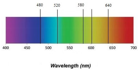
II. If in the sequence 3, 6, 8, 9, 12, 14, and 18, we calculate the distances between two consecutive terms, we obtain 3, 2, 1, 3, 2, and 4. We code this pattern by CBACBD, following the positions of letters in the English alphabet. Modeling some inherent approximations, this pattern appears in unexpected places. For example, in the visible spectrum, the colors span wavelength intervals, whose widthness (from right to left, i.e., from red to violet) are proportional to CBACBD, as shown in the next picture.
III. In the Mendeleev periodic table of elements, the pattern CFHILNR provides: (3)—Lithium (“Alkaline metals”), (6)—Carbon (“Other nonmetals”), (8)—Oxygen (“Other nonmetals”), (9)—Fluorine (“Halogens”), (12)—Magnesium (“Alkaline Earth metals”), (14)—Silicon (“Metalloids”), (18)—Argon (“Noble gases”). It is interesting that carbon, which is the basic element for life on Earth, corresponds to the singular Tsallis entropy constant 1; excluding it, the remaining six values provide elements in six distinct groups. By contrast, the following seven terms () in the fractal sequence give elements belonging to the (same) “Transition metals” group.
IV. In our paper, we worked with the Tsallis logarithm given in (8). In the literature, there exists also an additive dual (and equivalent) framework, which is based on a Tsallis logarithm of the form
Replacing , we obtain seven transformed (“dual”) “exceptional” parameters: . The first three are common with the previous list, as 1 is “auto-dual” and and are “dual” to each other.
Even if the new values also appear as “singular” ones in several applications, we did not succeed to establish for the new sequence any speculative link, which is similar to those in I, II and III. It is possible that this epistemological asymmetry indicates that the two (apparently equivalent) frameworks for the Tsallis logarithm are not “perfectly” equivalent, and that there might be some subtle/hidden properties which differentiate them.
V. Further study may include the analogue multiplicative dual approach of Tsallis [60], using the transformation . The algebraic theory of the Tsallis q-triplets was extended by means of more general Möbius transformations, depending on several parameters [60], such as
All these algebraic constructions were introduced with the expectation to create some order (and to decrease the “Entropy”) in the “Universe” of the Tsallis parameters. In our (speculative) opinion, one must take into account also “exceptional” values of the Tsallis entropy parameters, arising theoretically by algebraic and geometric invariants, as shown in Section 7.
References
- Bogachev, V.I.; Krylov, N.V.; Röckner, M.; Shaposhnikov, S.V. Fokker-Planck–Kolmogorov Equations; American Mathematical Society Mathematical Surveys and Monographs; American Mathematical Society: Providence, RI, USA, 2015; Volume 207. [Google Scholar]
- Kwok, S.F. Langevin and Fokker-Planck Equations and Their Generalizations; World Scientific: Singapore, 2018. [Google Scholar]
- Pavliotis, G.A. Stochastic Processes and Applications (Diffusion Processes, the Fokker-Planck and Langevin Equations); Springer: Berlin, Germany, 2014. [Google Scholar]
- Risken, H. The Fokker-Planck Equation (Methods of Solution and Applications), 3rd ed.; Springer: Berlin, Germany, 1996. [Google Scholar]
- Frank, T.D. Nonlinear Fokker-Planck Equations; Springer: Berlin/Heidelberg, Germany; New York, NY, USA, 2005. [Google Scholar]
- Barbu, V.; Röckner, M. Solutions for nonlinear Fokker-Planck equations with measures as initial data and McKean-Vlasov equations. J. Funct. Anal. 2021, 280, 108926. [Google Scholar] [CrossRef]
- Duan, C.; Chen, W.; Liu, C.; Wang, C.; Zhou, S. Convergence analysis of structure-preserving numerical methods for nonlinear Fokker-Planck equations with nonlocal interactions. Math. Methods Appl. Sci. 2022, 45, 3764–3781. [Google Scholar] [CrossRef]
- Fuentes, J.; Lopez, J.L.; Obregon, O. Generalized Fokker-Planck equations derived from nonextensive entropies asymptotically equivalent to Boltzmann-Gibbs. Phys. Rev. E 2020, 102, 012118. [Google Scholar] [CrossRef]
- Lima, L.S. Interplay between nonlinear Fokker-Planck equation and stochastic differential equation. Prob. Eng. Mech. 2022, 68, 103201. [Google Scholar] [CrossRef]
- Maarouf, N.; Hilal, K. Invariant analysis, analytical solutions, and conservation laws for two-dimensional time fractional Fokker-Planck equation. J. Funct. Spaces 2021, 2021, 2490392. [Google Scholar] [CrossRef]
- Millan, D.; Fonseca, F. The Solution of the Fokker-Planck Equation Using Lie Groups. Adv. Stud. Theor. Phys. 2017, 11, 477–485. [Google Scholar] [CrossRef]
- Peyghan, E.; Popescu, L. Geometric structures on Finsler Lie algebroids and applications to optimal control. Filomat 2022, 36, 39–71. [Google Scholar] [CrossRef]
- Plastino, A.R.; Wedemann, R.S. Nonlinear Fokker-Planck Equation Approach to Systems of Interacting Particles: Thermostatistical Features Related to the Range of the Interactions. Entropy 2020, 22, 163. [Google Scholar] [CrossRef] [Green Version]
- Ragusa, M.A.; Tachikawa, A. Regularity of minimizers of some variational integrals with discontinuity. Z. Anal. Ihre Anwend. 2008, 27, 469–482. [Google Scholar] [CrossRef]
- Ren, Y.A.; Yu, L.J.; Liao, J. The Hydrodynamic Limit of Nonlinear Fokker-Planck Equation. J. Appl. Math. Phys. 2020, 8, 2488–2499. [Google Scholar] [CrossRef]
- Zheng, J. Lie Symmetry Analysis and Invariant Solutions of a Nonlinear Fokker-Planck Equation Describing Cell Population Growth. Adv. Math. Phys. 2020, 2020, 4975943. [Google Scholar] [CrossRef]
- Olver, P.J. Applications of Lie Groups to Differential Equations; Springer: Berlin, Germany, 1986. [Google Scholar]
- Oliveri, F. Lie Symmetries of Differential Equations: Classical Results and Recent Contributions. Symmetry 2010, 2, 658–706. [Google Scholar] [CrossRef] [Green Version]
- Yaglom, I.M. Felix Klein and Sophus Lie: Evolution of the Idea of Symmetry in the Nineteenth Century; Birkhäuser: Boston, MA, USA, 1988. [Google Scholar]
- An, I.; Chen, S.; Guo, H.Y. Search for the symmetry of the Fokker-Planck equation. Physica A 1984, 128, 520–528. [Google Scholar] [CrossRef]
- Cicogna, G.; Vitali, D. Generalized symmetries of Fokker-Planck-type equations. J. Phys. A Math. Gen. 1989, 22, 453–456. [Google Scholar] [CrossRef]
- Cicogna, G.; Vitali, D. Classifications of the extended symmetries of Fokker-Planck-type equations. J. Phys. A Math. Gen. 1990, 23, 85–88. [Google Scholar] [CrossRef]
- Cicogna, G. Symmetries and (Related) Recursion Operators of Linear Evolution Equations. Symmetry 2010, 2, 98–111. [Google Scholar] [CrossRef]
- Scarfone, A.M.; Wada, T. Lie symmetries and related group-invariant solutions of a nonlinear Fokker-Planck equation based on the Sharma-Taneja-Mittal entropy. Braz. J. Phys. 2009, 39, 475–482. [Google Scholar] [CrossRef] [Green Version]
- Sinkala, W. Symmetry reductions and invariant solutions of a nonlinear Fokker-Planck equation based on the Sharma-Taneja-Mittal entropy. Int. J. Appl. Math. 2020, 33, 805–822. [Google Scholar] [CrossRef]
- Wada, T.; Scarfone, A.M. Asymptotic solutions of a nonlinear diffusive equation in the framework of a k-generalized statistical mechanics. Eur. Phys. J. B 2009, 70, 65–71. [Google Scholar] [CrossRef] [Green Version]
- Hirica, I.E.; Pripoae, C.-L.; Pripoae, G.-T.; Preda, V. Weighted Relative Group Entropies and Associated Fisher Metrics. Entropy 2022, 24, 120. [Google Scholar] [CrossRef]
- Tsallis, C. Nonadditive entropy and nonextensive statistical mechanics—An overview after 20 years. Braz. J. Phys. 2009, 39, 337–356. [Google Scholar] [CrossRef]
- Pripoae, C.-L.; Hirica, I.E.; Pripoae, G.-T.; Preda, V. Lie symmetries of the nonlinear Fokker-Planck equation based on weighted Tsallis entropy. Carpathian J. Math. 2022, 38, 597–617. [Google Scholar]
- Belis, M.; Guiasu, S. A quantitative-qualitative measure of informattion in cybernetic systems. IEEE Trans. Inf. Theory 1968, 14, 593–594. [Google Scholar] [CrossRef]
- Guiasu, S. Weighted entropy. Rep. Math. Phys. 1971, 2, 165–179. [Google Scholar] [CrossRef]
- Barbu, V.S.; Karagrigoriou, A.; Preda, V. Entropy and divergence rates for Markov chains: II. The weighted case. Proc. Rom. Acad. A 2018, 19, 3–10. [Google Scholar]
- Casquilho, J. Discussing an Expected Utility and Weighted Entropy Framework. Nat. Sci. 2014, 6, 545–551. [Google Scholar] [CrossRef] [Green Version]
- Kelbert, M.; Stuhl, I.; Suhov, I. Weighted entropy: Basic inequalities. Mod. Stoch. Theory Appl. 2017, 4, 233–252. [Google Scholar] [CrossRef] [Green Version]
- Mahdi, M. Weighted Entropy Measure: A New Measure of Information with its Properties in Reliability Theory and Stochastic Orders. J. Stat. Theory Appl. 2018, 17, 703–718. [Google Scholar] [CrossRef]
- Preda, V.; Balcau, C. Convex quadratic programming with weighted entropic perturbation. Bull. Math. Soc. Sci. Math. Roum. 2009, 52, 57–64. [Google Scholar]
- Smieja, M. Weighted approach to general entropy function. IMA J. Math. Control Inf. 2015, 32, 329–341. [Google Scholar]
- Stuhl, I.; Kelbert, M.; Suhov, Y.; Yasaei Sekeh, S. Weighted Gaussian entropy and determinant inequalities. Aequ. Math. 2022, 96, 85–114. [Google Scholar] [CrossRef]
- Gzyl, H. The Method of Maximum Entropy; World Scientific: Singapore, 1995. [Google Scholar]
- Kapur, J.N. Maximum-Entropy Models in Science and Engineering; John Wiley and Sons: New York, NY, USA, 1989. [Google Scholar]
- Ebrahimi, N.; Soofi, E.S.; Soyer, R. Multivariate maximum entropy identification, transformation and dependence. J. Multivar. Anal. 2008, 99, 1217–1231. [Google Scholar] [CrossRef] [Green Version]
- Fradkov, A.L.; Shalymov, D.S. Speed Gradient and MaxEnt Principles for Shannon and Tsallis Entropies. Entropy 2015, 17, 1090–1102. [Google Scholar] [CrossRef] [Green Version]
- Nielsen, F. MaxEnt upper bounds for the differential entropy of univariate continuous distributions. IEEE Signal Proc. Lett. 2017, 24, 402–406. [Google Scholar] [CrossRef]
- Preda, V. The Student distribution and the principle of maximum entropy. Ann. Inst. Stat. Math. 1982, 34, 335–338. [Google Scholar] [CrossRef]
- Wada, T.; Scarfone, A.M. On the non-linear Fokker-Planck equation associated with k-entropy. AIP Conf. Proc. 2007, 965, 177–180. [Google Scholar]
- Murdoch, I. Physical Foundations of Continuum Mechanics; Cambridge University Press: Cambridge, UK, 2012. [Google Scholar]
- Aggarwal, N.L.; Picard, C.F. Functional Equations and Information Measures with Preference. Kybernetika 1978, 14, 174–181. [Google Scholar]
- Giuclea, M.; Popescu, C.-C. On Geometric Mean and Cumulative Residual Entropy for Two Random Variables with Lindley Type Distribution. Mathematics 2022, 10, 1499. [Google Scholar] [CrossRef]
- Vogel, R.M. The geometric mean? Commun. Stat.—Theory Methods 2020, 51, 82–94. [Google Scholar] [CrossRef]
- Cover, T.M.; Thomas, J.A. Elements of Information Theory, 2nd ed.; Wiley-Interscience: Hoboken, NJ, USA, 2006. [Google Scholar]
- Mubarakzyanov, G.M. On solvable Lie algebras. Izv. Vyss. Uchebnykh Zaved. Mat. 1963, 32, 114–123. (In Russian) [Google Scholar]
- Bwanakare, S. Non-Extensive Entropy Econometrics: New Statistical Features of Constant Elasticity of Substitution-Related Models. Entropy 2014, 16, 2713–2728. [Google Scholar] [CrossRef] [Green Version]
- Niven, R.K. Constrained Forms of the Tsallis Entropy Function and Local Equilibria. arXiv 2005, arXiv:cond-mat/0503263. [Google Scholar]
- Pavlos, G.P.; Xenakis, M.N.; Karakatsanis, L.P.; Iliopoulos, A.C.; Pavlos, A.E.G.; Sarafopoulos, D.V. Universality of Tsallis Non-Extensive Statistics and Fractal Dynamics for Complex Systems. Chaotic Model. Simul. (CMSIM) 2012, 2, 395–447. [Google Scholar]
- Calderon, L.; Martin, M.T.; Plastino, A.; Rocca, M.C.; Vampa, V. Relativistic treatment of Verlinde’s emergent force in Tsallis’ statistics. Mod. Phys. Lett. A 2019, 34, 1950075. [Google Scholar] [CrossRef] [Green Version]
- Plastino, A.R.; Rocca, M.C. On the entropic derivation of the r-2 Newtonian gravity force. Phys. A Stat. Mech. Its Appl. 2017, 505, 190–195. [Google Scholar] [CrossRef] [Green Version]
- Furuichi, S. Some results on Tsallis entropies in classical system. Res. Inst. Math. Anal. 2007, 1561, 152–165. [Google Scholar]
- Furuichi, S. On the maximum entropy principle and the minimization of the Fisher information in Tsallis statistics. J. Math. Phys. 2009, 50, 013303. [Google Scholar] [CrossRef] [Green Version]
- Umarov, S.; Tsallis, C.; Steinberg, S. On a q-Central Limit Theorem Consistent with Nonextensive Statistical Mechanics. Milan J. Math. 2008, 76, 307–328. [Google Scholar] [CrossRef]
- Umarov, S.; Tsallis, C. Mathematical Foundations of Nonextensive Statistical Mechanics; World Scientific: Hackensack, NJ, USA, 2022. [Google Scholar]
- De la Cruz-García, J.S.; Bory-Reyes, J.; Ramirez-Arellano, A. A Two-Parameter Fractional Tsallis Decision Tree. Entropy 2022, 24, 572. [Google Scholar] [CrossRef] [PubMed]
- Sotolongo-Costa, O.; Rodriguez, A.H.; Rodgers, G.J. Tsallis Entropy and the transition to scaling in fragmentation. Entropy 2000, 2, 172–177. [Google Scholar] [CrossRef] [Green Version]
- Vilasini, V.; Colbeck, R. Analysing causal structures using Tsallis entropies. Phys. Rev. A 2019, 100, 062108. [Google Scholar] [CrossRef] [Green Version]
- Jizba, P.; Korbel, J. On q-non-extensive statistics with non-Tsallisian entropy. Physica A 2016, 444, 808–827. [Google Scholar] [CrossRef] [Green Version]
- Khusnutdinov, N.R.; Yulmetyev, R.M.; Emelyanova, N.A. Dynamic Tsallis Entropy for Simple Model Systems. Acta Phys. Pol. 2006, 109, 199–217. [Google Scholar] [CrossRef]
- Rebollo-Neira, L.; Plastino, A.; Fernandez-Rubio, J. On the q = non-extensive maximum entropy distribution. Physica A 1998, 258, 458–465. [Google Scholar] [CrossRef] [Green Version]
- Hirica, I.E.; Pripoae, C.-L.; Pripoae, G.-T.; Preda, V. Entropy—A Tale of Ice and Fire. in preparation.
Publisher’s Note: MDPI stays neutral with regard to jurisdictional claims in published maps and institutional affiliations. |
© 2022 by the authors. Licensee MDPI, Basel, Switzerland. This article is an open access article distributed under the terms and conditions of the Creative Commons Attribution (CC BY) license (https://creativecommons.org/licenses/by/4.0/).
Share and Cite
MDPI and ACS Style
Hirica, I.-E.; Pripoae, C.-L.; Pripoae, G.-T.; Preda, V. Lie Symmetries of the Nonlinear Fokker-Planck Equation Based on Weighted Kaniadakis Entropy. Mathematics 2022, 10, 2776. https://doi.org/10.3390/math10152776
AMA Style
Hirica I-E, Pripoae C-L, Pripoae G-T, Preda V. Lie Symmetries of the Nonlinear Fokker-Planck Equation Based on Weighted Kaniadakis Entropy. Mathematics. 2022; 10(15):2776. https://doi.org/10.3390/math10152776
Chicago/Turabian StyleHirica, Iulia-Elena, Cristina-Liliana Pripoae, Gabriel-Teodor Pripoae, and Vasile Preda. 2022. "Lie Symmetries of the Nonlinear Fokker-Planck Equation Based on Weighted Kaniadakis Entropy" Mathematics 10, no. 15: 2776. https://doi.org/10.3390/math10152776
Note that from the first issue of 2016, this journal uses article numbers instead of page numbers. See further details here.