
DL-Aided Underground Cavity Morphology Recognition Based on 3D GPR Data


School of Automation, Central South University, Changsha 410083, China
*
Author to whom correspondence should be addressed.
Mathematics 2022, 10(15), 2806; https://doi.org/10.3390/math10152806
Submission received: 27 June 2022
/
Revised: 29 July 2022
/
Accepted: 1 August 2022
/
Published: 8 August 2022
(This article belongs to the Special Issue Recent Advances in Swarm Intelligence Algorithms and Their Applications)
Abstract
:Cavity under urban roads has increasingly become a huge threat to traffic safety. This paper aims to study cavity morphology characteristics and proposes a deep learning (DL)-based morphology classification method using the 3D ground-penetrating radar (GPR) data. Fine-tuning technology in DL can be used in some cases with relatively few samples, but in the case of only one or very few samples, there will still be overfitting problems. To address this issue, a simple and general framework, few-shot learning (FSL), is first employed for the cavity classification tasks, based on which a classifier learns to identify new classes given only very few examples. We adopt a relation network (RelationNet) as the FSL framework, which consists of an embedding module and a relation module. Furthermore, the proposed method is simpler and faster because it does not require pre-training or fine-tuning. The experimental results are validated using the 3D GPR road modeling data obtained from the gprMax3D system. The proposed method is compared with other FSL networks such as ProtoNet, R2D2, and BaseLine relative to different benchmarks. The experimental results demonstrate that this method outperforms other prior approaches, and its average accuracy reaches 97.328% in a four-way five-shot problem using few support samples.
1. Introduction
Urban areas around the world continue to experience a series of sudden sinkhole collapses that cause severe traffic disruptions and significant economic losses. Underground cavities are the main reason for the formation of sinkholes. Complex conditions such as changes in drainage patterns, excessive pavement loads, and disturbances in infrastructure construction often lead to various cavities [1]. Therefore, the cavities may vary in morphology, for example, cavities with different shapes or combinations of several basic shapes, or they may be filled with different media or have different positions and sizes. Due to the unpredictability and morphological complexity of cavities, there is a growing need for their early recognition.
Ground-penetrating radar (GPR) has gradually been applied to the detection and perception of underground cavities [2], owing to its nondestructive inspection, strong penetrating ability, and high-precision characteristics. GPR transmitters emit electromagnetic (EM) waves into the surface at multiple spatial positions, and then the reflected signal can be measured by the GPR receiver to establish a two-dimensional (2D) GPR image. Three-dimensional (3D) GPR images can be obtained immediately when multichannel GPR transmitters and receivers exist parallel to the scanning direction at the same time [3,4]. The morphological scale of a cavity can reflect the evolution speed of the cavity and the severity of future road collapse, and it can also accurately reflect the 3D space state of the cavity. Therefore, the accurate detection of morphology has scientific value for studying the mechanism of cavity formation and summarizing the corresponding prevention and repair methods. However, as the quantity of the 3D GPR data increases, the manual analysis of the GPR data becomes time-consuming and difficult to meet the requirements of the efficient and fine detection of cavity morphology.
Three challenges in automating this task cannot be ignored. The first challenge is the selection and extraction of morphological features. Environmental complexities, such as the interference of surrounding pipelines and groundwater leakage, may impose difficulties in describing cavity morphological features. It is impossible to comprehensively describe the reflection properties with one or a few features. Additionally, the acquired morphological attributes still need to be inferred and identified by experienced professionals, making it difficult to obtain a general description feature. The second challenge is the fine classification of cavity morphology in the GPR data. Due to the variety of types, varying sizes, distinct directions and extensions, and irregular shapes, cavity morphology analysis faces difficulties in identification and fine classification. The third challenge is to address the issue of insufficiently labeled GPR data. Compared with objects such as buried rebars and pipes, the scale and diameter distribution of a cavity with collapse threat is relatively large. It is very laborious to make such a large target in the lab, and the targets are generally in regular forms, not universal and representative. To obtain reliable results, the lack of sample data must be considered and addressed.
Therefore, in this study, a novel deep learning (DL)-aided framework was proposed to extract the morphological features of cavities and classify them in facing a small number of 3D GPR data. Figure 1 shows the details of the proposed framework. The contribution of this work is twofold:
- (i)
- First, a joint characterization algorithm was developed for cavity morphology that generates 2D morphological images and fully exploits 3D GPR spatial information;
- (ii)
- Second, we implemented a novel few-shot learning (FSL) network for cavity morphology classification and embedded a relation network (RelationNet) into the FSL model to adapt to different few-sample cavity scenarios.
The rest of this paper is organized as follows: Section 2 introduces the literature review of the GPR cavity detection. In Section 3, the imaging scheme of the 3D GPR data is proposed. Section 4 introduces the details of the FSL network and RelationNet structure for morphological classification. In Section 5, the experimental results are compared and analyzed, and finally, in Section 6, conclusions are drawn.
2. Literature Review
Previous studies have focused on the automated GPR cavity detection process. Qin et al. [5] proposed a pattern recognition method based on the support vector machine (SVM) classifier to identify cavities in GPR images. Park et al. [6] combined instantaneous phase analysis with the GPR technique to identify hidden cavities. Hong et al. [7] developed a new time-domain-reflectometry-based penetrometer system to accurately estimate the relative permittivity at different depths and estimate the state of a cavity. Yang et al. [8] constructed a horizontal filter to identify cavity disease and eliminate the interference of rebar echo. Based on the data collected by multisensors such as unmanned aerial vehicles (UAVs) and GPR, the authors of [9,10] detected and analyzed cavity diseases in disaster-stricken areas to rescue potential victims trapped in cavities. In 2022, Rasol et al. [11] reviewed state-of-the-art processing techniques such as machine learning and intelligent data analysis methods, as well as their applications and challenges in GPR road pavement diagnosis. To better localize pavement cracks and solve the interference of various factors in the on-site scene, Liu et al. [12] integrated a ResNet50vd-deformable convolution backbone into YOLOv3, along with a hyperparameter optimization method. To detect subsurface road voids, Yamaguchi et al. [13] constructed a 3D CNN to extract hyperbolic reflection characteristics from GPR images.
Previous results were based on the processing of only B-scans; however, once faced with specific subsurface objects, it was difficult to classify them using B-scans alone. In particular, the characteristics of various cavities in GPR B-scan images tended to be similar. Therefore, to improve the classification performance, both the GPR B-scan and C-scan images were considered in the classification process using the DL network [14,15,16,17]. Compared with the 2D GPR data, 3D data can provide rich spatial information and greatly improve the process in terms of data volume, imaging methods, and disease detection accuracy. Luo et al. [18] established a cavity pattern database including C-scans and B-scans, where the C-scan provides location information of objects, and B-scan information assists in verifying object types. Kim et al. [19] proposed a triplanar convolutional neural network (CNN) for processing the 3D GPR data, enabling automated underground object classification. Kang et al. [20] designed the UcNet framework to reduce the misclassification of cavities, and the next year, Kang et al. [21] developed a transfer-enhanced CNN to improve the classification accuracy. Khudoyarov et al. [22] proposed a 3D CNN architecture to process the 3D GPR data. The authors of another study [23] visualized and distinguished underground hidden cavities from other objects (such as buried pipes, and manholes). In 2021, Kim et al. [24] used the AlexNet network with the transfer learning technology to achieve underground object classification, further improving detection accuracy and speed. Abhinaya et al. [25] detected cavities around sewers using in-pipe GPR equipment and confirmed that YOLOv3 [26] was suitable for cavity recognition tasks. Liu et al. [27] combined the YOLO model and the information embedded in 3D GPR images to address the recognition issue of road defects. The above research demonstrated that, compared with using only B-scan images, the developed CNNs using both the B-scans and C-scans improved the classification performance. However, it was found that the cavity morphology is still indistinguishable due to the difficulty of cavity data acquisition and the lack of a GPR database.
Faced with such a problem, FSL [28,29], as a novel DL technique, was developed to generalize the network with very few or fewer training samples for each class. This changes the situation where traditional DL models must require large quantities of labeled data. FSL can be divided into three categories: model-based, optimization-based, and metric-based learning methods [30]. The model-based learning method first designs the model structure and then uses the designed model to quickly update parameters on a small number of samples, and finally directly establishes the mapping function of the input and prediction values. Santoro et al. [31] proposed the use of memory augmentation to solve this task and a memory-based neural network approach to adjust bias through weight updates. Munkhdalai et al. [32] proposed a meta-learning network, and its fast generalization ability is derived from the “fast weight” mechanism, where the gradients generated during training are used for fast weight generation. The optimization-based learning method completes the task of small sample classification by adjusting the optimization method instead of the conventional gradient descent method. Based on the fact that gradient-based optimization algorithm does not work well with a small quantity of data, Ravi et al. [33] studied an updated function or rule for model parameters. The method proposed by Finn et al. [34] can deal with situations with a small number of samples and can obtain better model generalization performance with only a small number of training times. The main advantages of this method are that it does not depend on the model form, nor does it need to add new parameters to the meta-learning network. The metric-based learning method is developed to measure the distance/similarity between the training set and the support set and completes the classification with the help of the nearest neighbor method. Vinyals et al. [35] proposed a new matching network, which aims to build different encoders for the support set and the batch set, respectively. Sung et al. [36] proposed a RelationNet network to model the measurement method, which learns the distance measurement method by training a CNN network.
3. Imaging Scheme of 3D GPR Data
3.1. The 3D GPR Data Format
The GPR data comes in three forms: A-, B-, and C-scan. The transmitter radiates EM waves to the underground, and the receiver collects signals reflected by underground objects or stratum interfaces, so as to obtain underground information. The original data format of the reflected signal is a one-dimensional (1D) waveform, which can also be called a GPR A-scan waveform. By scanning a region of interest with the single-channel GPR system, a 2D radargram can be obtained, called a GPR B-scan image. A single C-scan image is formed by imaging data points at the same depth in multiple B-scan images.
As shown in Figure 2, the x-axis is the same as the scanning direction, the y-axis denotes the width direction of the radar antenna device, and the z-axis indicates the depth direction of the measured object. The 3D GPR data can be represented as two kinds of orthogonal planes: B-scan and C-scan. B-scan and C-scan are arbitrary sections perpendicular to y- and z-axes. This is conducive to identifying the cavity morphology from multiple different perspectives, which can effectively avoid the misjudgment of a single angle in the 2D image. Therefore, 3D GPR can guarantee the accuracy of the detection type and reduce the number of core sampling verifications.
3.2. GPR Morphological Data Extraction
The hyperbolic signature in B-scan images is a kind of typical characteristic that is often used in the detection of underground objects. The C-scan image can reflect the detailed shape information of the subsurface cavity. The B-scan and C-scan images contain morphological information in length–depth and length–width directions, respectively. The color on scan images reflects the field strength (V/m) of subsurface media. In this study, we propose an automatic algorithm for cavity morphology classification using GPR B-scan and C-scan images simultaneously.
The two forms are extracted from the 3D GPR data . Take the irregular cavity as an example: (1) B-scan images are sequentially extracted parallel to the XOZ plane, and their stacked display is shown in Figure 3a. It can be expressed as , , where represents each slice image, is a collection of B-scan slices, , and are the model space length and space step size in the y-axis direction. (2) C-scan images are sequentially extracted parallel to the XOY plane. The horizontal slices are extracted at equal intervals, and their stacked display is shown in Figure 3b. The slices can be expressed as , , where represents each C-scan image, is the set of C-scan slices, and are the model space length and space step size in the z-axis direction.
The typical GPR B-scan and the corresponding C-scan images of an irregular cavity are shown in Figure 4 and Figure 5. The C-scan images (right) are intersectional layers of red lines on the B-scan images (left). In the B-scan image, the horizontal x-axis and the vertical t-axis indicate the GPR scanning trajectory (m) and the two-way travel time of EM wave (ns), respectively. In the C-scan image, the x- and y-axes indicate the GPR scanning trajectory (m) and the width of GPR equipment (m), respectively. As shown in Figure 4, the irregular cavity shows a hyperbolic pattern on the B-scan image and elliptical signatures on the C-scan image. As shown in Figure 5, the rectangular cavity shows a double hyperbolic signature on the B-scan image and quadrilateral signatures (Figure 5b) on the C-scan images. Therefore, different morphologies of cavities can be well-recognized using B-scan and C-scan images.
3.3. The 2D Morphological Image Generation
Multiple B-scan and C-scan images are integrated into a 2D morphological map, where the B-scan and C-scan images are assigned to the upper and lower parts of the morphological map, respectively. Each cavity model corresponds to a 2D morphological image , which consists of 8 B-scan images , and 12 C-scan images . The morphological image consists of and , which is formed into a new matrix and can also be expressed as Equation (1). Examples of the morphological images for each model are presented in Figure 6. The 2D morphological image is then used as the input of the following deep network.
4. Few-Shot Learning Designed for Morphology Classification
4.1. FSL Definition
FSL is able to quickly identify new classes on very few samples. It is generally divided into three kinds of datasets: training set, support set, and testing set. The training set can be further divided into a sample set and a query set. If the support set contains labeled examples for each of unique classes, the target few-shot problem is called -way -shot. Figure 7 shows the FSL architecture for a four-way one-shot problem.
The parameters are optimized by the training set, hyperparameters are tuned using the support set, and finally, the performance of function is evaluated on the test set. Each sample is assigned a class label . The data structure in the training phase is constructed to be similar to that in the testing phase; that is, the sample set and query set during the training simulate the support set and testing set at the testing time. The sample set is built by randomly picking classes from the training set with labeled samples, and the rest of these samples are used in the query set .
4.2. Relation Network Architecture and Relation Score Computation
The relation network (RelationNet) is a typical metric-learning-based FSL method. In essence, metric-learning-based methods [36,37,38,39,40,41] compare the similarities between query images and support classes through a feed-forward pass through an episodic training mechanism [35]. The core of RelationNet is to learn a nonlinear metric through deep CNN, rather than selecting a fixed metric function. RelationNet is a two-branch architecture that includes an embedding module and a relation module. The embedding module is used to extract image features. The relation module obtains the correlation score between query images and sample images; that is, it measures their similarity, so as to realize the recognition task of a small number of samples.
Figure 8 represents the RelationNet architecture settings for FSL. The embedding module utilizes four convolutional blocks, and each convolutional block consists of a 64-filter convolution, a batch normalization, and a ReLU nonlinearity layer. In addition to the above, the first two convolutional blocks also include a max-pooling layer, and the latter two convolutional blocks do not contain the pooling layer. The output feature maps are then obtained for the following convolutional layers in the relation module. The relation module consists of two convolutional blocks and two fully connected layers. Each convolutional block is a convolution containing 64 filters, followed by batch normalization, ReLU nonlinearity, and max-pooling. For the network architectures, in order to generate relation scores within a reasonable range, in all fully connected layers, ReLU functions are employed, except for the output layer, in which Sigmoid is used.
The prior few-shot works use fixed pre-specified distance metrics, such as the Euclidean or cosine distances, to perform classification [35,42]. Compared with the previously used fixed metrics, RelationNet can be viewed as a metric capable of learning deep embeddings and deep nonlinearities. By learning the similarity using a flexible function approximator, RelationNet can better identify matching/mismatching pairs. Sample in the query set and sample in the sample set are fed through the embedding module to produce feature maps and , respectively. Then, these two feature maps and are combined using the operator . After that, the combined feature map is fed into the relation module , which finally produces a scalar in the range of 0–1 to represent the similarity between and , also called the relation score. Thus, the relation score is generated as shown in Equation (2):
Here, the mean square error loss is computed to train the model, as shown in Equation (3), regressing the relation score to the ground truth: the similarity of matched pairs is 1, and the similarity of unmatched pairs is 0.
4.3. RelationNet-Based Cavity Morphology Classification Scheme
Based on the data and structural characteristics of the GPR cavity morphological recognition system, we divide the complex processing process into two main parts: a training phase and a testing phase, as shown in Figure 9. The cavity morphologies are discussed here, e.g., cylindrical, rectangular, spherical, and irregular hemispherical. First, a training set is inputted to learn classification rules inside the network in the training phase. Then, in the testing phase, a small number of support samples (labeled) and test samples (unlabeled) are inputted into the trained network model, and the unlabeled test samples are predicted and classified, thereby outputting the final morphological classification results.
Based on the above principle, the RelationNet-based GPR cavity morphology classification system first obtains the trained model on the training set and then recognizes the new category of cavity images. The embedding model is used to extract the feature information of each inputted GPR image and then concatenates the image features between the test sample and support sample. Then, the integrated features are inputted into the relation model for comparison. According to the comparison results, it is judged to which category the test sample belongs, so as to achieve the classification of cavity morphologies.
5. Experiments and Results
5.1. Experimental Settings
The classification category should be labeled for each morphological image since the DL-based classification algorithm is essentially a supervised learning algorithm. The choice of category is related to the morphology of the cavity. There are four types of cavities involved, namely cylindrical cavity, rectangular cavity, spherical cavity, and irregular cavity. To train CNN, the 2D morphological images with each image size of 498 × 395 × 3 pixels were fed to the input layer, and then the convolutional layers were used to extract multilevel image features by convolution kernels. A total of 68 GPR morphological images were obtained, each consisting of 8 B-scans and 12 C-scans. Among them, there were 17 spherical cavity images, 17 cylindrical cavity images, 17 rectangular cavity images, and 17 irregular cavity images.
We used the PyTorch 1.5 implementations of the LibFewShot package [43], which is a comprehensive FSL library and integrates the most advanced FSL methods. The code was implemented using NVIDIA RTX 3080Ti GPU and Intel i9-12900K CPU. In the training phase, in the FSL in all experiments, we used the Adam optimizer [44] with an initial learning rate of 10−3 and step decay. The backbone adopted Conv64F. The batch size was set to 128. In the testing phase, the test epoch was set to 10, and the test episode was 17, the four-way one-shot contained 16 query images, and the four-way five-shot had 12 query images for each of the 4 classes in each training episode.
We compared the results against those of various networks for few-shot recognition, including ProtoNet [42], R2D2 [45], and BaseLine [46]. Embedding backbones, such as Conv64F, ResNet12, and ResNet18, were also compared to identify and select the main backbone with a better performance. The main experiments were conducted on two benchmark datasets: miniImageNet [35] and tieredImageNet [47]. The miniImageNet dataset [35] consists of 60,000 color images with 100 classes, and the input images are resized to 84 × 84. The tieredImageNet dataset [47] consists of 779,165 color images with 608 classes, each of size 84 × 84.
5.2. The 3D GPR Cavity Data Acquisition
The GPR data are difficult to collect and label. To address the issue, a 3D GPR forward modeling tool, GprMax3D [48,49], is often used for the 3D modeling and simulation of underground structures. Based on the finite-difference time-domain (FDTD) method, the technique increases the volume of training data by creating synthetic GPR images. Maxwell’s equations govern the propagation of EM waves used by the GPR. Figure 10 shows the flowchart of the GprMax3D forward simulation technique. GprMax3D was used to generate synthetic GPR images [50]. To further imitate the real situation, we set up cavity objects with uneven surfaces and random media to approximate real objects. An example of the GPR system’s parameter setting is shown in Table 1.
Road cavity is generally distributed in the underground range of 0.3–1 m, which is also the junction of the pavement structure and the subgrade. The subgrade is generally a soil structure, while the pavement structure is generally a flexible, semi-rigid, or rigid structure, generally made of cement or asphalt concrete; in particular, its bottom layer is generally made of hard materials such as gravel. Due to the high probability of soil erosion, cavities are most likely to appear at the junction of soft and hard layers. Figure 11 shows a simulation model example of a road structure with the first layer of asphalt, the second layer of concrete, and the third layer of sandstone. Their attribute parameter settings are shown in Table 2. In addition, the subgrade is generally dominated by soil, and a more realistic soil model was established by simulating random media. A number of soil dispersion materials were defined as follows: soil with 50% sand, 50% clay, sand density of 2.66 g/cm3, clay bulk density of 2 g/cm3, and volumetric water content ranging from 0.001 to 0.25. These materials were distributed over a model with a volume of m3 (in which the soil layers were randomly distributed).
Figure 12 presents the simulated models of four representative cavity morphologies: spherical, rectangular, cylindrical, and irregular hemispherical cavities. The first three cavities have smooth surfaces, and the last one shows an uneven surface. Figure 13 shows the representative 2D GPR morphological images of cavities. Figure 13a shows the case of spherical cavities with parabolic and circular features, which can be observed on the B-scan and C-scan images, respectively. As shown in Figure 13b, rectangular cavities generally have distinguishable features, namely a double parabola shape in B-scans. Similar features are also revealed in the cylindrical case of Figure 13c. However, Figure 13b,c can be distinguished by C-scans because they, respectively, show quadrilateral signatures and double circular intersection features in C-scans. Compared with Figure 13a, it can be observed in Figure 13d that the C-scan images of the irregular cavity show unsmoothed circular features with considerable noise randomly distributed inside the circle. Due to these distinguishable and representative characteristics, the cavity morphology can be classified well with the FSL frameworks.
5.3. Classification Results and Analysis
Figure 14 shows the RelationNet-based underground cavity morphology classification results. These results were obtained based on the network settings of the backbone Conv64F, the benchmark dataset tieredImageNet, and in a four-way five-shot problem. As expected, compared with the ground truth, the irregular hemispherical cavity with significant characteristics in the GPR morphological image was correctly classified. Moreover, the classification accuracy rates of spherical, rectangular, and cylindrical cavities were 97.5%, 98.33%, and 98.33%, respectively. However, 0.83% and 1.67% of spherical were misclassified as cylindrical and hemispherical due to their similar morphological features. In addition, 1.67% of rectangular were misclassified as hemispherical due to their double parabola shapes in B-scans, while 0.83% and 0.83% of cylindrical were, respectively, misclassified as spherical and hemispherical, due to their similar features in B- or C-scans. The classification performance of RelationNet was evaluated based on the indices (precision, recall, and F-score) using the following Equations (4)–(6):
Table 3 shows the statistical results obtained from the RelationNet results, namely the precision, recall, and F-score values. For the rectangular cases, 99.15% precision and 97.5% recall indicated that false-positive (FP) and false-negative (FN) results occurred, and the number of FN results was greater than those of FP. Similarly, the 99.16% precision and 98.33% recall values of the cylindrical case meant the FP and FN alarms because RelationNet sometimes recognized a cylindrical cavity as a spherical or hemispherical. For rectangular cases, 100% precision and the relatively low recall value indicated that FN occurred due to the misclassification between rectangular and hemispherical. On the contrary, 96% precision and 100% recall values meant that the hemispherical samples were properly classified using RelationNet, but multiple samples in other categories were misclassified as hemispherical at the same time. According to the F-scores, it can be concluded that the performance of RelationNet was acceptable.
5.4. Comparison Experiments
5.4.1. RelationNet Evaluation on Different Embedding Backbones
The performance of RelationNet relies on the quality of the embedding backbone. To select a suitable main embedding backbone, we compared three different embedding backbones: Conv64F, ResNet12, and ResNet18. The above experiments were run for 10 epochs on the miniImageNet dataset. Other settings remained the same. Conv64F consisted of four convolutional blocks, and each block was composed of a convolutional layer, a batch-normalization layer, a ReLU layer, and a max-pooling layer. ResNet12 consisted of four residual blocks, each of which contained three convolutional blocks along with a skip connection layer. ResNet18 had the same architecture as used in [50]. Table 4 shows the comparison results among different backbones. It can be observed that RelationNet equipped with Conv64F backbone achieved the best performance in either a four-way one-shot or four-way five-shot problem.
5.4.2. RelationNet Evaluation on Different Benchmark Datasets
Table 5 compares the performance of RelationNet on miniImageNet and tieredImageNet datasets by controlling the most implementation details. For this comparison, RelationNet adopted Conv64F as the main backbone. As can be seen from Table 5, in the four-way one-shot problem, the accuracy achieved on the miniImageNet dataset was slightly higher than that on the tieredImageNet dataset. In the four-way five-shot problem, competitive accuracy could be achieved using the tieredImageNet dataset compared with using the miniImageNet dataset, improving the accuracy by 8.394%. Therefore, the accuracy results indicated that RelationNet performed well when trained on the tieredImageNet dataset.
5.4.3. Performance Comparison of Different FSL Networks
To validate the effectiveness of RelationNet, the four experimental validation results of ProtoNet, R2D2, BaseLine, and RelationNet were compared. We used the exact same embedding backbone Conv64F and benchmark dataset miniImageNet. It can be observed from Table 6 that RelationNet achieved the best results in the four-way one-shot problem, even improving the accuracy by 11.994% over the BaseLine. With the increase in the number of sample images, these four frameworks achieved substantial improvements in facing the four-way five-shot problem, and RelationNet still achieved the highest accuracy over the other three frameworks.
6. Conclusions
In this paper, we first applied the FSL technique to classify and identify cavity morphology characteristics based on the 3D GPR data. RelationNet was adopted as the FSL framework and trained end-to-end from scratch. Based on the advantages of learning a deep distance metric, RelationNet addressed the issue of insufficient cavity data and obtained the classification results using only a few samples. The experiment results demonstrated the effectiveness of using RelationNet in morphology classification performance. The RelationNet model achieved an average classification accuracy value of 97.328% in the four-way five-shot and 78.097% in the four-way one-shot problem.
There is a limitation that could be addressed in future research. In the experiments, all the models were trained on the source domain (e.g., miniImageNet and tieredImageNet) and directly tested on the target domain (e.g., cavity radar dataset). However, the performance hardly improved or significantly dropped when there was a large domain shift. In this paper, based on the fact that there was no intersection between the source set and our cavity radar dataset, there was a large domain offset between the source and target domains. Future efforts need to be made to integrate prior knowledge into FSL or explore one-shot or zero-shot classification methods.
For on-site applications, there are two limitations that could be addressed in future research. First, the real cavity data are difficult to collect for training the proposed method. Additionally, the publicly available GPR cavity datasets are limited. Efforts need to be made in the future to collect and prepare GPR datasets to facilitate the implementation of this method. Second, the proposed method was only tested for cavity morphology classification using the GprMax3D data. The scalability of the method in other challenging environments and applications needs further investigation. Future studies could test this method for collecting cavity data and classifying their morphologies in on-site city roads.
Author Contributions
F.H.: Conceptualization, Methodology, Writing—Original Draft Preparation, Software. X.L.: Data Curation, Writing, Validation. X.F.: Visualization, Investigation. Y.G.: Supervision, Writing—Reviewing and Editing. All authors have read and agreed to the published version of the manuscript.
Funding
This work was funded by the National Natural Science Foundation of China (no. 61871407).
Institutional Review Board Statement
Not applicable.
Conflicts of Interest
The authors declare no conflict of interest.
References
- Gutiérrez, F.; Parise, M.; Waele, J.; Jourde, H. A review on natural and human-induced geohazards and impacts in karst. Earth Sci. Rev. 2014, 138, 61–88. [Google Scholar]
- Garcia-Garcia, F.; Valls-Ayuso, A.; Benlloch-Marco, J.; Valcuende-Paya, M. An optimization of the work disruption by 3D cavity mapping using GPR: A new sewerage project in Torrente (Valencia, Spain). Constr. Build. Mater. 2017, 154, 1226–1233. [Google Scholar] [CrossRef] [Green Version]
- Jol, H.M. Ground Penetrating Radar Theory and Applications; Elseviere: Amsterdam, The Netherlands, 2008. [Google Scholar]
- Meyers, R.; Smith, D.; Jol, H.; Peterson, C. Evidence for eight great earthquake-subsidence events detected with ground-penetrating radar, Willapa barrier, Washington. Geology 1996, 24, 99–102. [Google Scholar] [CrossRef]
- Qin, Y.; Huang, C. Identifying underground voids using a GPR circular-end bow-tie antenna system based on a support vector machine. Int..J. Remote Sens. 2016, 37, 876–888. [Google Scholar] [CrossRef]
- Park, B.; Kim, J.; Lee, J.; Kang, M.-S.; An, Y.-K. Underground object classification for urban roads using instantaneous phase analysis of Ground-Penetrating Radar (GPR) Data. Remote Sens. 2018, 10, 1417. [Google Scholar] [CrossRef] [Green Version]
- Hong, W.-T.; Lee, J.-S. Estimation of ground cavity configurations using ground penetrating radar and time domain reflectometry. Nat. Hazards 2018, 92, 1789–1807. [Google Scholar] [CrossRef]
- Yang, Y.; Zhao, W. Curvelet transform-based identification of void diseases in ballastless track by ground-penetrating radar. Struct. Control Health Monit. 2019, 26, e2322–e2339. [Google Scholar] [CrossRef]
- Chen, J.; Li, S.; Liu, D.; Li, X. AiRobSim: Simulating a Multisensor Aerial Robot for Urban Search and Rescue Operation and Training. Sensors 2020, 20, 5223–5242. [Google Scholar] [CrossRef] [PubMed]
- Hu, D.; Li, S.; Chen, J.; Kamat, V.R. Detecting, locating, and characterizing voids in disaster rubble for search and rescue. Adv. Eng. Inform. 2019, 42, 100974–100982. [Google Scholar] [CrossRef]
- Rasol, M.; Pais, J.; Pérez-Gracia, V.; Solla, M.; Fernandes, F.; Fontul, S.; Ayala-Cabrera, D.; Schmidt, F.; Assadollahi, H. GPR monitoring for road transport infrastructure: A systematic review and machine learning insights. Constr. Build. Mate. 2022, 324, 126686. [Google Scholar] [CrossRef]
- Liu, Z.; Gu, X.; Yang, H.; Wang, L.; Chen, Y.; Wang, D. Novel YOLOv3 Model With Structure and Hyperparameter Optimization for Detection of Pavement Concealed Cracks in GPR Images. IEEE T Intell. Transp. Syst. 2022, 1, 1–11. [Google Scholar] [CrossRef]
- Yamaguchi, T.; Mizutani, T.; Meguro, K.; Hirano, T. Detecting Subsurface Voids From GPR Images by 3-D Convolutional Neural Network Using 2-D Finite Difference Time Domain Method. IEEE J. Sel. Top. Appl. Earth Obs. Remote Sens. 2022, 15, 3061–3073. [Google Scholar] [CrossRef]
- Yamashita, Y.; Kamoshita, T.; Akiyama, Y.; Hattori, H.; Kakishita, Y.; Sadaki, T.; Okazaki, H. Improving efficiency of cavity detection under paved road from GPR data using deep learning method. In Proceedings of the 13th SEGJ International Symposium, Tokyo, Japan, 12–14 November 2018; Society of Exploration Geophysicists and Society of Exploration Geophysicists of Japan: Tykyo, Japan, 2019; pp. 526–529. [Google Scholar]
- Ni, Z.-K.; Zhao, D.; Ye, S.B.; Fang, G. City road cavity detection using YOLOv3 for ground-penetrating radar. In Proceedings of the18th International Conference on Ground Penetrating Radar, Golden, CO, USA, 14–19 June 2020; Society of Exploration Geophysicists: Houston, TX, USA, 2020; pp. 2159–6832. [Google Scholar]
- Liu, H.; Shi, Z.; Li, J.; Liu, C.; Meng, X.; Du, Y.; Chen, J. Detection of road cavities in urban cities by 3D ground-penetrating radar. Geophysics 2021, 86, WA25–WA33. [Google Scholar] [CrossRef]
- Feng, J.; Yang, L.; Hoxha, E.; Xiao, J. Improving 3D Metric GPR Imaging Using Automated Data Collection and Learning-based Processing. IEEE Sens. J. 2022, 1–13. [Google Scholar] [CrossRef]
- Luo, T.; Lai, W. GPR pattern recognition of shallow subsurface air voids. Tunn. Undergr. Sp. Tech. 2020, 99, 103355–103366. [Google Scholar] [CrossRef]
- Kim, N.; Kim, S.; An, Y.-K.; Lee, J.-J. Triplanar imaging of 3-D GPR data for deep-learning-based underground object detection. IEEE J. Sel. Top. Appl. Earth Obs. Remote Sens. 2019, 12, 4446–4456. [Google Scholar] [CrossRef]
- Kang, M.-S.; Kim, N.; Im, S.B.; Lee, J.-J.; An, Y.-K. 3D GPR image-based UcNet for enhancing underground cavity detectability. Remote Sens. 2019, 11, 2545–2562. [Google Scholar] [CrossRef] [Green Version]
- Kang, M.-S.; Kim, N.; Lee, J.-J.; An, Y.-K. Deep learning-based automated underground cavity detection using three-dimensional ground penetrating radar. Struct. Health Monit. 2020, 19, 173–185. [Google Scholar] [CrossRef]
- Khudoyarov, S.; Kim, N.; Lee, J.-J. Three-dimensional convolutional neural network–based underground object classification using three-dimensional ground penetrating radar data. Struct. Health Monit. 2020, 19, 1884–1893. [Google Scholar] [CrossRef]
- Kim, N.; Kim, K.; An, Y.-K.; Lee, H.-J.; Lee, J.-J. Deep learning-based underground object detection for urban road pavement. Int. J. Pavement Eng. 2020, 21, 1638–1650. [Google Scholar] [CrossRef]
- Kim, N.; Kim, S.; An, Y.-K.; Lee, J.-J. A novel 3D GPR image arrangement for deep learning-based underground object classification. Int. J. Pavement Eng. 2021, 22, 740–751. [Google Scholar] [CrossRef]
- Abhinaya, A. Using Machine Learning to Detect Voids in an Underground Pipeline Using in-Pipe Ground Penetrating Radar. Master’s Thesis, University of Twente, Enschede, Holland, 2021. [Google Scholar]
- Redmon, J.; Farhadi, A. Yolov3: An incremental improvement. arXiv 2018, arXiv:1804.02767. [Google Scholar]
- Liu, Z.; Wu, W.; Gu, X.; Li, S.; Wang, L.; Zhang, T. Application of combining YOLO models and 3D GPR images in road detection and maintenance. Remote Sens. 2021, 13, 1081–1099. [Google Scholar] [CrossRef]
- Lu, J.; Gong, P.; Ye, J.; Zhang, C. Learning from very few samples: A survey. arXiv 2020, arXiv:2009.02653. [Google Scholar]
- Yang, S.; Liu, L.; Xu, M. Free lunch for few-shot learning: Distribution calibration. arXiv 2021, arXiv:2101.06395. [Google Scholar]
- Wang, Y.; Yao, Q.; Kwok, J.; Ni, L. Generalizing from a few examples: A survey on few-shot learning. ACM Comput. Surv. 2020, 53, 1–34. [Google Scholar] [CrossRef]
- Santoro, A.; Bartunov, S.; Botvinick, M.; Wierstra, D.; Lillicrap, T. One-shot learning with memory-augmented neural networks. arXiv 2016, arXiv:1605.06065. [Google Scholar]
- Munkhdalai, T.; Yu, H. Meta networks. In Proceedings of the International Conference on Machine Learning, Sydney, Australia, 6–17 August 2017. [Google Scholar]
- Ravi, S.; Larochelle, H. Optimization as a model for few-shot learning. In Proceedings of the International Conference on Learning Representations (ICLR), Toulon, France, 24–26 April 2017. [Google Scholar]
- Finn, C.; Abbeel, P.; Levine, S. Model-agnostic meta-learning for fast adaptation of deep networks. In Proceedings of the International Conference on Machine Learning, Sydney, Australia, 6–17 August 2017. [Google Scholar]
- Vinyals, O.; Blundell, C.; Lillicrap, T.; Kavukcuoglu, K.; Wierstra, D. Matching networks for one shot learning. Adv. Neural Inf. Process. Syst. 2016, 29, 3630–3638. [Google Scholar]
- Sung, F.; Yang, Y.; Zhang, L.; Xiang, T.; Torr, P.; Hospedales, T. Learning to compare: Relation network for few-shot learning. In Proceedings of the IEEE conference on computer vision and pattern recognition, Salt Lake City, UT, USA, 18–22 June 2018; pp. 1199–1208. [Google Scholar]
- Koch, G.; Zemel, R.; Salakhutdinov, R. Siamese neural networks for one-shot image recognition. ICML Deep. Learn. Workshop 2015, 2, 2015. [Google Scholar]
- Li, W.; Wang, L.; Xu, J.; Huo, J.; Gao, Y.; Luo, J. Revisiting local descriptor based image-to-class measure for few-shot learning. In Proceedings of the IEEE/CVF Conference on Computer Vision and Pattern Recognition, California, CA, USA, 16–20 June 2019; pp. 7260–7268. [Google Scholar]
- Wertheimer, D.; Tang, L.; Hariharan, B. Few-shot classification with feature map reconstruction networks. In Proceedings of the IEEE/CVF Conference on Computer Vision and Pattern Recognition, Nashville, TN, USA, 19–25 June 2021; pp. 8012–8021. [Google Scholar]
- Kang, D.; Kwon, H.; Min, J.; Cho, M. Relational Embedding for Few-Shot Classification. In Proceedings of the IEEE/CVF International Conference on Computer Vision, Montreal, QC, Canada, 11–17 October 2021; pp. 8822–8833. [Google Scholar]
- Zhang, C.; Cai, Y.; Lin, G.; Shen, C. Deepemd: Few-shot image classification with differentiable earth mover’s distance and structured classifiers. In Proceedings of the IEEE/CVF conference on computer vision and pattern recognition, Seattle, WA, USA, 13–19 June 2020; pp. 12203–12213. [Google Scholar]
- Snell, J.; Swersky, K.; Zemel, R. Prototypical networks for few-shot learning. Adv. Neural Inf. Process. Syst. 2017, 30, 1–11. [Google Scholar]
- Li, W.; Dong, C.; Tian, P.; Qin, T.; Yang, X.; Wang, Z.; Huo, J.; Shi, Y.; Wang, L.; Gao, Y.; et al. LibFewShot: A Comprehensive Library for Few-shot Learning. arXiv 2021, arXiv:2109.04898. [Google Scholar]
- Kingma, D.; Ba, J. Adam: A method for stochastic optimization. arXiv 2014, arXiv:1412.6980. [Google Scholar]
- Bertinetto, L.; Henriques, J.; Torr, P.; Vedaldi, A. Meta-learning with differentiable closed-form solvers. arXiv 2018, arXiv:1805.08136. [Google Scholar]
- Chen, W.-Y.; Liu, Y.-C.; Kira, Z.; Wang, Y.-C.; Huang, J.-B. A closer look at few-shot classification. arXiv 2019, arXiv:1904.04232. [Google Scholar]
- Ren, M.; Triantafillou, E.; Ravi, S.; Snell, J.; Swersky, K.; Tenenbaum, J.; Larochelle, H.; Zemel, R. Meta-learning for semi-supervised few-shot classification. arXiv 2018, arXiv:1803.00676, 2018. [Google Scholar]
- Warren, C.; Giannopoulos, A.; Giannakis, I. gprMax: Open source software to simulate electromagnetic wave propagation for ground penetrating radar. Comput. Phys. Commun. 2016, 209, 163–170. [Google Scholar] [CrossRef] [Green Version]
- Giannakis, I.; Giannopoulos, A.; Warren, C. A realistic FDTD numerical modeling framework of ground penetrating radar for landmine detection. IEEE J. Sel. Top. Appl. Earth Obs. Remote Sens. 2016, 9, 37–51. [Google Scholar] [CrossRef]
- He, K.; Zhang, X.; Ren, S.; Sun, J. Deep residual learning for image recognition. In Proceedings of the IEEE conference on computer vision and pattern recognition, Las Vegas, NV, USA, 27–30 June 2016; pp. 770–778. [Google Scholar]
Figure 1.
GPR cavity morphology recognition framework.
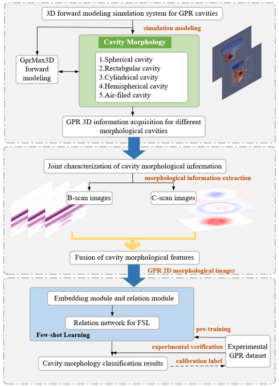
Figure 2.
Orthogonal slice planes (B-, C-scan) of 3D GPR data.

Figure 3.
Sacked morphological images extracted from an irregular cavity: (a) stacked B-scan images; (b) stacked C-scan images.
Figure 3.
Sacked morphological images extracted from an irregular cavity: (a) stacked B-scan images; (b) stacked C-scan images.
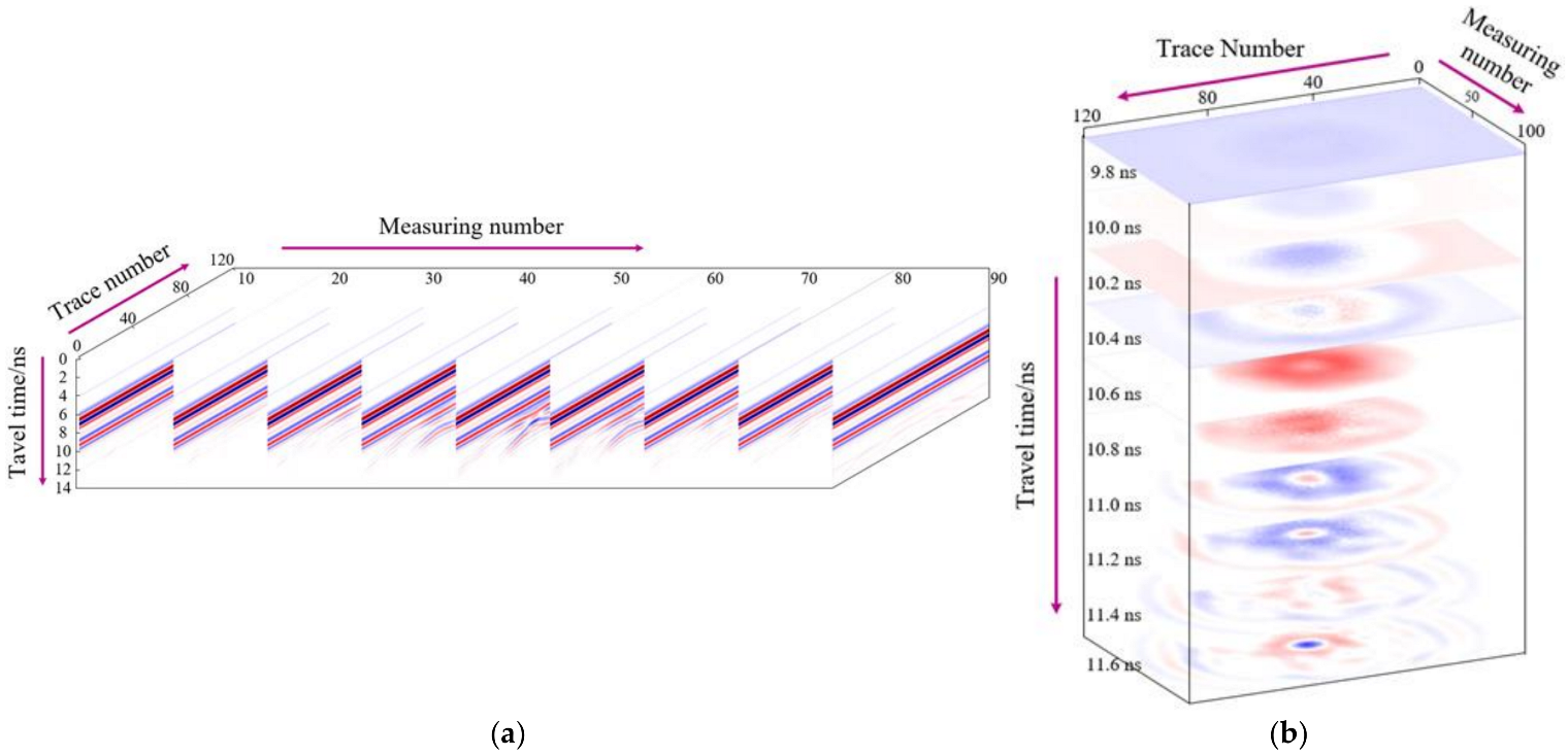
Figure 4.
Typical GPR images of an irregular cavity: (a) B-scan image; (b) C-scan images.

Figure 5.
Typical GPR images of a rectangular cavity: (a) B-scan image; (b) C-scan images.
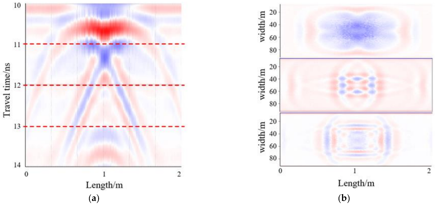
Figure 6.
The 2D GPR morphological images of (a) a spherical cavity, (b) a rectangular cavity, (c) a cylindrical cavity, and (d) an irregular cavity.
Figure 6.
The 2D GPR morphological images of (a) a spherical cavity, (b) a rectangular cavity, (c) a cylindrical cavity, and (d) an irregular cavity.

Figure 7.
FSL architecture for a four-way one-shot problem with one query example.
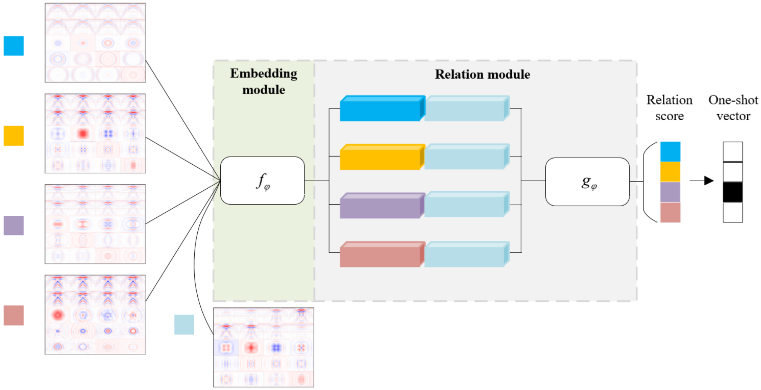
Figure 8.
RelationNet architecture settings.
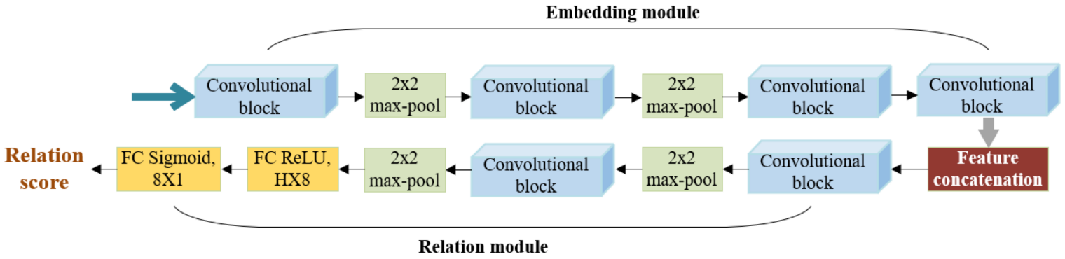
Figure 9.
RelationNet-based GPR cavity morphology classification scheme.
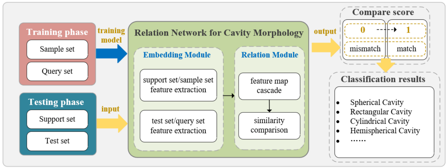
Figure 10.
GprMax3D simulation flowchart.

Figure 11.
Road structural simulation model.

Figure 12.
Display of simulation model from different perspectives (cavity in red).
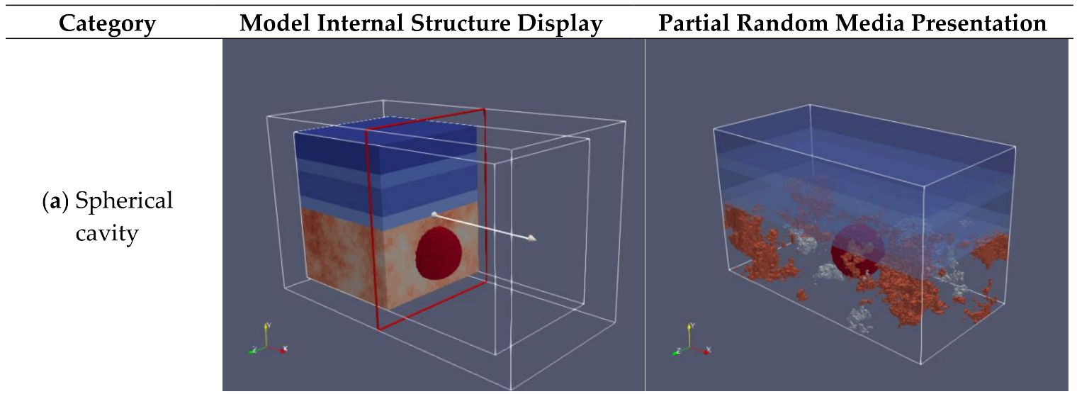
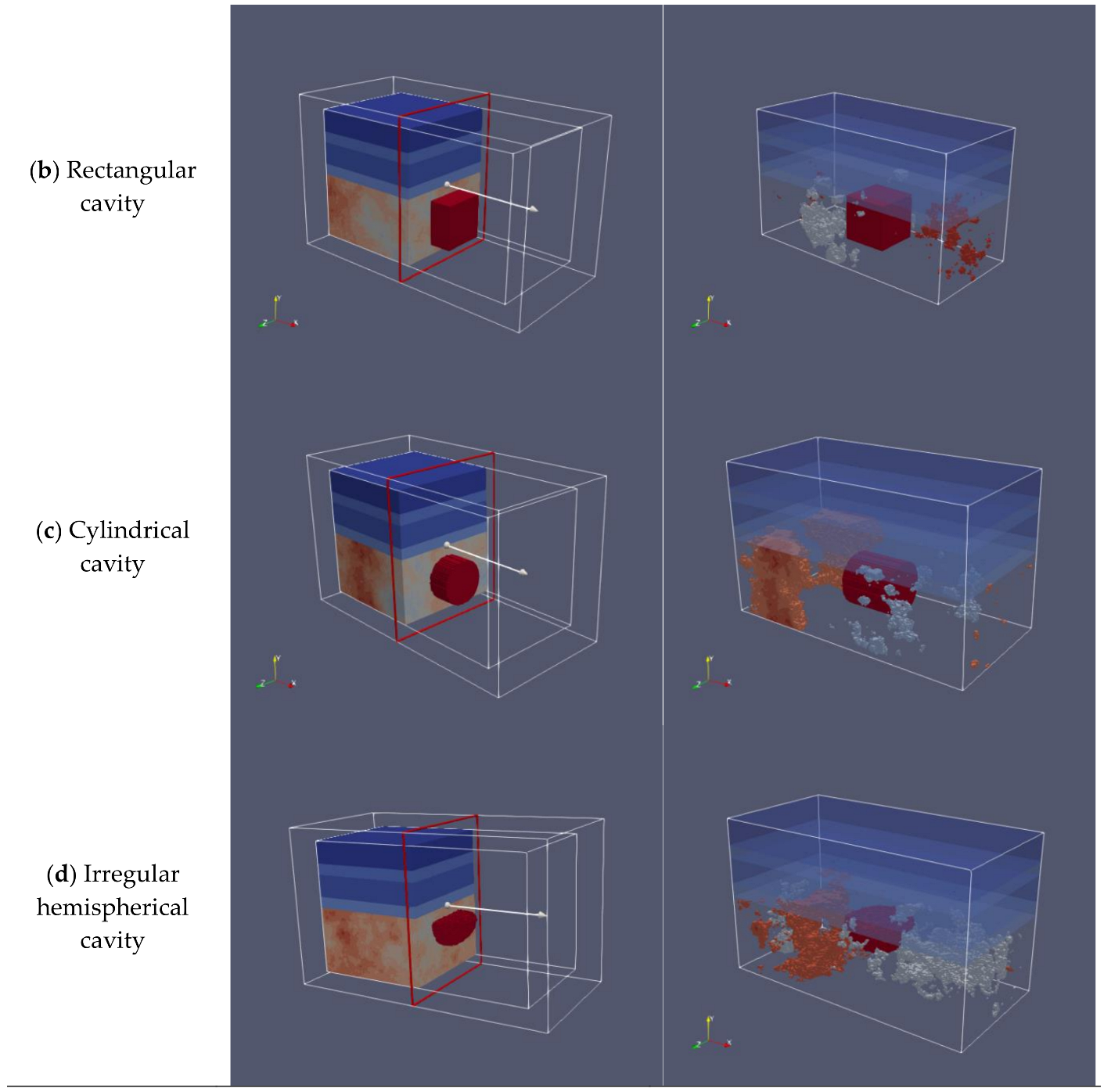
Figure 13.
Representative 2D GPR images of cavities: (a) spherical, (b) rectangular, (c) cylindrical, and (d) irregular hemispherical.
Figure 13.
Representative 2D GPR images of cavities: (a) spherical, (b) rectangular, (c) cylindrical, and (d) irregular hemispherical.
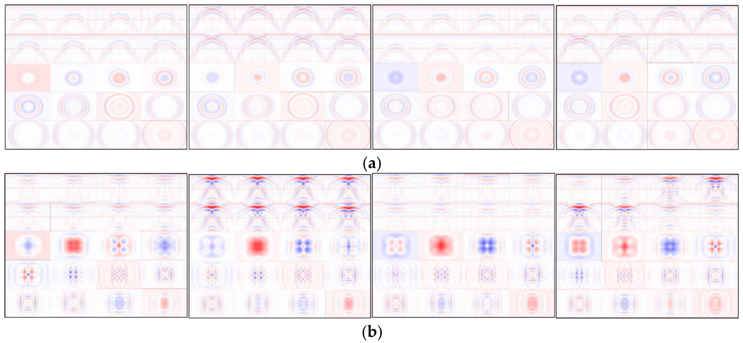

Figure 14.
The results of RelationNet-based cavity morphological classification.


Table 1.
GPR system parameters in road structure scene.
| System Parameters | Value |
|---|---|
| Spatial resolution/m | 0.01 |
| Time window/ns | 14 |
| Initial coordinate of transmit antenna/m | (0.45, 1.0, 0.0) |
| Initial coordinate of receive antenna/m | (0.35, 1.0, 0.0) |
| Antenna step distance/m | (0.01, 0, 0) |
| Measuring point number | 100 |
| Excitation signal type | Ricker |
| Excitation signal frequency/MHz | 800 |
Table 2.
Dielectric properties of road structure.
| System Parameters | Relative Permittivity | Conductivity (S/m) |
|---|---|---|
| Air | 1 | 0 |
| Asphalt | 6 | 0.005 |
| Concrete (dry) | 9 | 0.05 |
| Gravel | 12 | 0.1 |
Table 3.
Statistical results obtained from RelationNet (%).
| System Parameters | Precision | Recall | F-Score |
|---|---|---|---|
| Spherical | 99.15 | 97.5 | 98.32 |
| Rectangular | 100 | 98.33 | 99.16 |
| Cylindrical | 99.16 | 98.33 | 98.74 |
| Hemispherical | 96 | 100 | 97.96 |
Table 4.
Comparison results on different embedding backbones (%) (the best results in bold).
| Embedding Backbones | Four-Way One-Shot | Four-Way Five-Shot |
|---|---|---|
| Conv64F | 78.097 | 88.934 |
| ResNet12 | 69.467 | 72.500 |
| ResNet18 | 69.926 | 79.865 |
Table 5.
Comparison results on different benchmark datasets: miniImageNet vs. tieredImageNet (%) (the best results in bold).
Table 5.
Comparison results on different benchmark datasets: miniImageNet vs. tieredImageNet (%) (the best results in bold).
| Embedding Backbones | Four-Way One-Shot | Four-Way Five-Shot |
|---|---|---|
| miniImageNet | 78.097 | 88.934 |
| tieredImageNet | 77.086 | 97.328 |
Table 6.
Statistical results obtained from RelationNet (%) (the best results in bold).
| FSL Networks | Four-Way One-Shot | Four-Way Five-Shot |
|---|---|---|
| ProtoNet | 70.965 | 85.221 |
| R2D2 | 76.562 | 88.659 |
| BaseLine | 66.103 | 83.505 |
| RelationNet | 78.097 | 88.934 |
Publisher’s Note: MDPI stays neutral with regard to jurisdictional claims in published maps and institutional affiliations. |
© 2022 by the authors. Licensee MDPI, Basel, Switzerland. This article is an open access article distributed under the terms and conditions of the Creative Commons Attribution (CC BY) license (https://creativecommons.org/licenses/by/4.0/).
Share and Cite
MDPI and ACS Style
Hou, F.; Liu, X.; Fan, X.; Guo, Y. DL-Aided Underground Cavity Morphology Recognition Based on 3D GPR Data. Mathematics 2022, 10, 2806. https://doi.org/10.3390/math10152806
AMA Style
Hou F, Liu X, Fan X, Guo Y. DL-Aided Underground Cavity Morphology Recognition Based on 3D GPR Data. Mathematics. 2022; 10(15):2806. https://doi.org/10.3390/math10152806
Chicago/Turabian StyleHou, Feifei, Xu Liu, Xinyu Fan, and Ying Guo. 2022. "DL-Aided Underground Cavity Morphology Recognition Based on 3D GPR Data" Mathematics 10, no. 15: 2806. https://doi.org/10.3390/math10152806
Note that from the first issue of 2016, this journal uses article numbers instead of page numbers. See further details here.