
Analysis of Stochastic State-Dependent Arrivals in a Queueing-Inventory System with Multiple Server Vacation and Retrial Facility


 , ,
, ,  , and
, and 
Abstract
:1. Introduction
1.1. Motivation
1.2. Contribution of the Model
- 1.
- This model analyses the state-dependent arrival pattern on the expected system performance measures.
- 2.
- This model brings out the stability condition and the stationary probability vector of the proposed system using the Neuts matrix analytic method.
- 3.
- Using numerical simulation, it investigates the expected total cost of the model under parameter variation.
- 4.
- The fraction of time of a server’s vacation is to be discussed in detail with a numerical illustration.
- 5.
- The customer’s waiting time, the fraction of successful rate of retrial, the expected mean inventory level, the number of customers in the waiting hall, thes and orbit are to be analysed using the parameter variation.
1.3. Literature Review
1.4. Research Gap
1.5. Proposal of the Model
- 1.
- A server status-dependent arrival rate is assumed for both primary and retrial arrivals in a vacation queueing-inventory system.
- 2.
- The server vacation offer is utilised only when both zero stock and zero customers in the queue occur.
- 3.
- Multiple server vacation policy is assumed.
- 4.
- In addition, the ordering principle is adopted for the replenishment of the inventory.
- 5.
- If the waiting hall is full, an arriving new customer sends to an infinite orbit or leaves the system under the Bernoulli schedule.
2. Model Definition
2.1. Model Explanation
2.2. Matrix Formulation
3. Main Results
3.1. Stability Analysis
3.2. Steady State Analysis
3.3. Computation of R-Matrix
4. System Performance Measures
- 1.
- Mean number of Iitems in the Inventory
- 2.
- Mean reorder rate
- 3.
- Probability that the server is on vacation
- 4.
- Probability that the server is busy
- 5.
- Probability that the server is idle
- 6.
- Overall rate of retrial
- 7.
- Successful rate of retrial
- 8.
- Fraction of successful retrial rate
- 9.
- Mean number of customers in the waiting hall
- 10.
- Mean number of customers arriving into the waiting hall
- 11.
- Average waiting time for the customer in the waiting hall
- 12.
- Mean number of customers in the orbit
- 13.
- Mean number of customers arriving into the orbit
- 14.
- Waiting time for the customer in the orbit
Total Cost Analysis
5. Numerical Examples
- 1.
- We observe that the total cost increases whenever and increase. Since the arrival rate is increasing, there will be a higher number of customers arriving in the waiting hall. Thus, the total cost will be increased along with the waiting cost.
- 2.
- The retrial rates and impact the total cost by reducing it as they increase. This is because, when the retrial rate is increased, customers leave the orbit. Thus the product value of and the waiting cost for them is decreased, and this will yield the decreases of the total cost.
- 3.
- It is clear that the total cost decreases as the service rate μ increases. As μ increases, the average service time per customer is decreased, and the waiting hall size is also decreased simultaneously. Therefore, the waiting cost for the at the time is decreased, which causes the decrease in the total cost.
- 4.
- Observing the result, we come to know that if the vacation completion rate increases, the respective total decreases. This is because the duration of the server being on vacation decreases as γ increases, and the server will be available to provide service to the customers. In this situation, the number of customers in the waiting hall will decrease. Then the waiting cost for the at the time will decrease that yields reduce of total cost.
- 5.
- It is known that total cost increases as N increases. This is because, when the waiting hall size is increased, will be increased. So the product value of the and the waiting cost for them increases the total cost.
- 6.
- Whenever the reorder rate β increases, the total cost decreases. This means the average replenishment time is decreased when β increases. Therefore, the setup cost per order is decreased, which causes a decrease in the total cost.
- 1.
- From Table 2, the average waiting time of customers in the waiting hall and orbit increases as the arrival rates and increase, because more number of customers will be arriving at the waiting hall due to the increment in the arrival rates. Similarly, when and increase, the customer in the orbit increases. This results in an increase in waiting time for the primary and orbital customers.
- 2.
- It is clear that the increases and the number of customers in the the orbit decreases if the retrial rates and increase. This causes an increase in the average waiting time for the customer in the waiting hall and a decrease in the average waiting time for the customer in the orbit.
- 3.
- While increasing the service rate μ, the average service time per customer is increased in Table 3. Consequently, the number of customers in the waiting hall as well as in the orbit has decreased. So the average waiting time of both customers has decreased.
- 4.
- We observe that the average waiting time of the primary and retrial customers reduces when the reorder rate is increased. In this case, the mean reorder time is decreased. That results in a decrease in the . Similarly, the number of customers in orbit also decreases. This explains the decrease in the average waiting time of both customers as β increases.
- 5.
- One part of the average waiting time of a customer always depends upon the waiting hall size. Increasing the waiting hall size increases , which increases the waiting time of customers in the waiting hall. For the retrial customers, as there are more place in the waiting hall, decreases. So the waiting time of customers in the orbit decreases while increasing N.

| 2 | 2.5 | 3 | 9 | 10.5 | 12 | ||||||
|---|---|---|---|---|---|---|---|---|---|---|---|
| 0.4 | 4 | 1.16049626 | 1.15994888 | 1.15967796 | 2.5 | 1.566933 | 1.274744 | 1.088836 | |||
| 3.3 | 5 | 1.60073258 | 1.59847405 | 1.59737999 | 4 | 4 | 1.564398 | 1.272200 | 1.086288 | ||
| 6 | 2.20734817 | 2.20021918 | 2.19679518 | 5.5 | 1.563741 | 1.271203 | 1.085071 | ||||
| 4 | 1.16051381 | 1.15996627 | 1.15969530 | 2.5 | 1.578102 | 1.275889 | 1.087037 | ||||
| 3.5 | 5 | 1.60079059 | 1.59853154 | 1.59743728 | 1.8 | 5 | 4 | 1.575629 | 1.273390 | 1.084524 | |
| 6 | 2.20748564 | 2.20035502 | 2.19693028 | 5.5 | 1.575577 | 1.272823 | 1.083637 | ||||
| 4 | 1.16053124 | 1.15998354 | 1.15971251 | 2.5 | 1.589663 | 1.279158 | 1.087767 | ||||
| 3.7 | 5 | 1.60084824 | 1.59858862 | 1.59749416 | 6 | 4 | 1.587715 | 1.276695 | 1.085279 | ||
| 6 | 2.20762226 | 2.20048991 | 2.19706439 | 5.5 | 1.587242 | 1.276489 | 1.084668 | ||||
| 0.6 | 4 | 1.16049626 | 1.15994887 | 1.15967794 | 2.5 | 1.566922 | 1.274731 | 1.088822 | |||
| 3.3 | 5 | 1.60073247 | 1.59847384 | 1.59737974 | 4 | 4 | 1.564333 | 1.272129 | 1.086212 | ||
| 6 | 2.20734703 | 2.20021770 | 2.19679362 | 5.5 | 1.563282 | 1.270707 | 1.084546 | ||||
| 4 | 1.16051380 | 1.15996626 | 1.15969528 | 2.5 | 1.578088 | 1.275874 | 1.087021 | ||||
| 3.5 | 5 | 1.60079049 | 1.59853134 | 1.59743705 | 2.05 | 5 | 4 | 1.575555 | 1.273311 | 1.084440 | |
| 6 | 2.20748455 | 2.20035359 | 2.19692878 | 5.5 | 1.575071 | 1.272280 | 1.083068 | ||||
| 4 | 1.16053123 | 1.15998353 | 1.15971249 | 2.5 | 1.589648 | 1.279142 | 1.087749 | ||||
| 3.7 | 5 | 1.60084814 | 1.59858843 | 1.59749393 | 6 | 4 | 1.587167 | 1.276609 | 1.085189 | ||
| 6 | 2.20762122 | 2.20048854 | 2.19706295 | 5.5 | 1.587160 | 1.275906 | 1.084059 | ||||
| 0.8 | 4 | 1.16049625 | 1.15994885 | 1.15967791 | 2.5 | 1.566913 | 1.274721 | 1.088812 | |||
| 3.3 | 5 | 1.60073235 | 1.59847360 | 1.59737946 | 4 | 4 | 1.564285 | 1.272077 | 1.086156 | ||
| 6 | 2.20734581 | 2.20021609 | 2.19679192 | 5.5 | 1.562947 | 1.270345 | 1.084165 | ||||
| 4 | 1.16051379 | 1.15996625 | 1.15969526 | 2.5 | 1.578078 | 1.275863 | 1.087010 | ||||
| 3.5 | 5 | 1.60079037 | 1.59853111 | 1.59743678 | 2.3 | 5 | 4 | 1.575502 | 1.273253 | 1.084379 | |
| 6 | 2.20748338 | 2.20035205 | 2.19692715 | 5.5 | 1.574705 | 1.271889 | 1.082657 | ||||
| 4 | 1.16053122 | 1.15998352 | 1.15971247 | 2.5 | 1.589636 | 1.279129 | 1.087736 | ||||
| 3.7 | 5 | 1.60084803 | 1.59858821 | 1.59749368 | 6 | 4 | 1.587101 | 1.276546 | 1.085124 | ||
| 6 | 2.20762009 | 2.20048706 | 2.19706139 | 5.5 | 1.586773 | 1.275488 | 1.083623 | ||||
| 4 | 5 | 6 | ||||||
|---|---|---|---|---|---|---|---|---|
| WT | WTO | WT | WTO | WT | WTO | |||
| 3.3 | 0.1640018 | 0.601369 | 0.1914943 | 0.603069 | 0.2267440 | 0.605800 | ||
| 2 | 3.5 | 0.1640039 | 0.601379 | 0.1914997 | 0.603077 | 0.2267548 | 0.605805 | |
| 3.7 | 0.1640060 | 0.601388 | 0.1915051 | 0.603085 | 0.2267655 | 0.605811 | ||
| 3.3 | 0.1641697 | 0.501025 | 0.1919572 | 0.502266 | 0.2278050 | 0.504274 | ||
| 0.4 | 2.5 | 3.5 | 0.1641718 | 0.501036 | 0.1919628 | 0.502275 | 0.2278162 | 0.504280 |
| 3.7 | 0.1641739 | 0.501045 | 0.1919683 | 0.502283 | 0.2278271 | 0.504285 | ||
| 3.3 | 0.1643207 | 0.434139 | 0.1923805 | 0.435084 | 0.2287917 | 0.436624 | ||
| 3 | 3.5 | 0.1643228 | 0.434149 | 0.1923862 | 0.435093 | 0.2288031 | 0.436630 | |
| 3.7 | 0.1643249 | 0.434159 | 0.1923918 | 0.435101 | 0.2288143 | 0.436636 | ||
| 3.3 | 0.1640019 | 0.601351 | 0.1914947 | 0.603039 | 0.2267454 | 0.605758 | ||
| 2 | 3.5 | 0.1640040 | 0.601361 | 0.1915001 | 0.603048 | 0.2267562 | 0.605764 | |
| 3.7 | 0.1640060 | 0.601371 | 0.1915055 | 0.603056 | 0.2267668 | 0.605770 | ||
| 3.3 | 0.1641697 | 0.501012 | 0.1919575 | 0.502244 | 0.2278062 | 0.504243 | ||
| 0.6 | 2.5 | 3.5 | 0.1641719 | 0.501023 | 0.1919631 | 0.502253 | 0.2278173 | 0.504250 |
| 3.7 | 0.1641739 | 0.501033 | 0.1919686 | 0.502262 | 0.2278282 | 0.504256 | ||
| 3.3 | 0.1643207 | 0.434129 | 0.1923808 | 0.435068 | 0.2287927 | 0.436601 | ||
| 3 | 3.5 | 0.1643229 | 0.434139 | 0.1923865 | 0.435077 | 0.2288041 | 0.436607 | |
| 3.7 | 0.1643250 | 0.434150 | 0.1923921 | 0.435085 | 0.2288152 | 0.436614 | ||
| 3.3 | 0.1640020 | 0.601335 | 0.1914950 | 0.603012 | 0.2267466 | 0.605719 | ||
| 2 | 3.5 | 0.1640041 | 0.601346 | 0.1915005 | 0.603021 | 0.2267574 | 0.605726 | |
| 3.7 | 0.1640061 | 0.601356 | 0.1915058 | 0.603030 | 0.2267680 | 0.605732 | ||
| 3.3 | 0.1641698 | 0.501000 | 0.1919578 | 0.502224 | 0.2278073 | 0.504215 | ||
| 0.8 | 2.5 | 3.5 | 0.1641719 | 0.501011 | 0.1919634 | 0.502234 | 0.2278183 | 0.504222 |
| 3.7 | 0.1641740 | 0.501021 | 0.1919689 | 0.502243 | 0.2278292 | 0.504229 | ||
| 3.3 | 0.1643208 | 0.434120 | 0.1923810 | 0.435052 | 0.2287937 | 0.436579 | ||
| 3 | 3.5 | 0.1643229 | 0.434130 | 0.1923867 | 0.435062 | 0.2288050 | 0.436586 | |
| 3.7 | 0.1643251 | 0.434141 | 0.1923923 | 0.435071 | 0.2288161 | 0.436593 | ||
| 2.5 | 4 | 5.5 | ||||||
|---|---|---|---|---|---|---|---|---|
| WT | WTO | WT | WTO | WT | WTO | |||
| 4 | 9 | 0.208426 | 0.517491 | 0.207456 | 0.516128 | 0.207370 | 0.515991 | |
| 1.8 | 10.5 | 0.160917 | 0.500893 | 0.160030 | 0.498722 | 0.159947 | 0.498502 | |
| 12 | 0.130799 | 0.489298 | 0.129960 | 0.485964 | 0.129879 | 0.485622 | ||
| 9 | 0.208354 | 0.517346 | 0.207446 | 0.516107 | 0.207368 | 0.515987 | ||
| 2.05 | 10.5 | 0.160842 | 0.500620 | 0.160019 | 0.498682 | 0.159945 | 0.498494 | |
| 12 | 0.130721 | 0.488828 | 0.129949 | 0.485893 | 0.129877 | 0.485609 | ||
| 9 | 0.208207 | 0.517077 | 0.207425 | 0.516067 | 0.207364 | 0.515980 | ||
| 2.3 | 10.5 | 0.160691 | 0.500134 | 0.159997 | 0.498608 | 0.159941 | 0.498480 | |
| 12 | 0.130566 | 0.488010 | 0.129926 | 0.485767 | 0.129873 | 0.485585 | ||
| 5 | 9 | 0.214582 | 0.514856 | 0.213481 | 0.513138 | 0.213381 | 0.512962 | |
| 1.8 | 10.5 | 0.164254 | 0.499808 | 0.163257 | 0.496706 | 0.163164 | 0.496390 | |
| 12 | 0.132765 | 0.490032 | 0.131829 | 0.484682 | 0.131739 | 0.484134 | ||
| 9 | 0.214499 | 0.514650 | 0.213469 | 0.513107 | 0.213379 | 0.512956 | ||
| 2.05 | 10.5 | 0.164168 | 0.499361 | 0.163245 | 0.496637 | 0.163161 | 0.496376 | |
| 12 | 0.132677 | 0.489167 | 0.131816 | 0.484545 | 0.131736 | 0.484106 | ||
| 9 | 0.214439 | 0.514510 | 0.213460 | 0.513085 | 0.213378 | 0.512952 | ||
| 2.3 | 10.5 | 0.164106 | 0.499064 | 0.163236 | 0.496590 | 0.163160 | 0.496367 | |
| 12 | 0.132612 | 0.488597 | 0.131807 | 0.484453 | 0.131735 | 0.484088 | ||
| 6 | 9 | 0.218524 | 0.514227 | 0.217311 | 0.512080 | 0.217201 | 0.511860 | |
| 1.8 | 10.5 | 0.166129 | 0.500579 | 0.165043 | 0.496164 | 0.164941 | 0.495718 | |
| 12 | 0.133756 | 0.493127 | 0.132744 | 0.484633 | 0.132646 | 0.483756 | ||
| 9 | 0.218432 | 0.513941 | 0.217298 | 0.512034 | 0.217198 | 0.511850 | ||
| 2.05 | 10.5 | 0.166034 | 0.499867 | 0.165029 | 0.496049 | 0.164938 | 0.495695 | |
| 12 | 0.133658 | 0.491602 | 0.132729 | 0.484373 | 0.132643 | 0.483704 | ||
| 9 | 0.218366 | 0.513755 | 0.217288 | 0.512003 | 0.217196 | 0.511844 | ||
| 2.3 | 10.5 | 0.165965 | 0.499413 | 0.165019 | 0.495975 | 0.164936 | 0.495680 | |
| 12 | 0.133587 | 0.490635 | 0.132719 | 0.484207 | 0.132641 | 0.483670 | ||
- 1.
- While the server is on vacation, the fraction of time the server is on vacation decreases as the arrival rate increases. While increasing , the number of customers in the waiting hall increases. So the customer’s arrival during the server’s vacation leads the server to work. Thus, the possibility of the server being on vacation decreases.
- 2.
- While increasing the arrival rate of customers during the server’s normal mode, the fraction of time the server being on vacation increases. As increases, the number of primary customers increases in the waiting hall, which leads to stock-out frequently and the server going on vacation frequently.
- 3.
- The fraction of time the server is on vacation decreases if the arrival rate of retrial customers during the server’s vacation increases. Because the increases due to the increase of . So the customer’s arrival in the waiting hall during vacation leads the server to work Â.
- 4.
- Â As increases, the number of customers increases in the waiting hall, which leads to stock-out often, and the server goes on vacation frequently, such that the fraction of time the server is on vacation increases.
- 5.
- Since the service rate increases, the fraction of time that the server is on vacation increases. Due to the increment in the rate μ, and items in the inventory decrease. So, the server can take a vacation frequently.
- 6.
- Whenever the replenishment rate increases, the fraction of time a server is on vacation decreases. If we increase the value of β, the replenishment time is decreased. So server has to work for more time, which decreases the fraction of time the server is on vacation.
- 7.
- By increasing the vacation completion rate, the fraction of time a server is on vacation decreases. Since the rate γ increases, the duration of server on vacation is decreased. So the server has to return to the normal mode often, which confirms the decrease in the fraction of time the server is on vacation.
- 8.
- The number of customers in the waiting hall increases upon increasing the waiting hall size, which leads to a stock out often as more customers can be accommodated in the waiting hall. So the possibility of a server taking a vacation is as high as inventory.
| 2 | 2.5 | 3 | 9 | 10.5 | 12 | ||||||
|---|---|---|---|---|---|---|---|---|---|---|---|
| 4 | 0.0000671 | 0.0000673 | 0.0000675 | 2.5 | 0.0008935 | 0.0010153 | 0.0011096 | ||||
| 3.3 | 5 | 0.0002016 | 0.0002022 | 0.0002027 | 4 | 4 | 0.0001142 | 0.0001320 | 0.0001461 | ||
| 6 | 0.0004277 | 0.0004285 | 0.0004289 | 5.5 | 0.0000196 | 0.0000232 | 0.0000262 | ||||
| 4 | 0.0000667 | 0.0000669 | 0.0000671 | 2.5 | 0.0008958 | 0.0010187 | 0.0011130 | ||||
| 0.4 | 3.5 | 5 | 0.0002004 | 0.0002011 | 0.0002016 | 1.8 | 5 | 4 | 0.0001187 | 0.0001361 | 0.0001497 |
| 6 | 0.0004253 | 0.0004261 | 0.0004265 | 5.5 | 0.0000214 | 0.0000249 | 0.0000277 | ||||
| 4 | 0.0000663 | 0.0000665 | 0.0000667 | 2.5 | 0.0008965 | 0.0010202 | 0.0011144 | ||||
| 3.7 | 5 | 0.0001993 | 0.0002000 | 0.0002005 | 6 | 4 | 0.0001212 | 0.0001383 | 0.0001515 | ||
| 6 | 0.0004230 | 0.0004238 | 0.0004242 | 5.5 | 0.0000225 | 0.0000259 | 0.0000285 | ||||
| 4 | 0.00006704 | 0.0000673 | 0.0000674 | 2.5 | 0.0008093 | 0.0009198 | 0.0010053 | ||||
| 3.3 | 5 | 0.00020147 | 0.0002022 | 0.0002027 | 4 | 4 | 0.0001029 | 0.0001190 | 0.0001317 | ||
| 6 | 0.00042734 | 0.0004282 | 0.0004286 | 5.5 | 0.0000176 | 0.0000209 | 0.0000235 | ||||
| 4 | 0.00006666 | 0.0000669 | 0.0000671 | 2.5 | 0.0008115 | 0.0009230 | 0.0010084 | ||||
| 0.6 | 3.5 | 5 | 0.00020033 | 0.0002010 | 0.0002015 | 2.05 | 5 | 4 | 0.0001070 | 0.0001227 | 0.0001350 |
| 6 | 0.00042496 | 0.0004258 | 0.0004262 | 5.5 | 0.0000192 | 0.0000224 | 0.0000249 | ||||
| 4 | 0.00006630 | 0.0000665 | 0.0000667 | 2.5 | 0.0008123 | 0.0009244 | 0.0010097 | ||||
| 3.7 | 5 | 0.00019925 | 0.0001999 | 0.0002004 | 6 | 4 | 0.0001092 | 0.0001247 | 0.0001366 | ||
| 6 | 0.00042270 | 0.0004235 | 0.0004239 | 5.5 | 0.0000202 | 0.0000232 | 0.0000256 | ||||
| 4 | 0.0000670 | 0.0000673 | 0.0000674 | 2.5 | 0.0007435 | 0.0008450 | 0.0009236 | ||||
| 3.3 | 5 | 0.0002014 | 0.0002021 | 0.0002026 | 4 | 4 | 0.0000941 | 0.0001088 | 0.0001204 | ||
| 6 | 0.0004270 | 0.0004279 | 0.0004284 | 5.5 | 0.0000161 | 0.0000190 | 0.0000214 | ||||
| 4 | 0.0000666 | 0.0000669 | 0.0000670 | 2.5 | 0.0007456 | 0.0008481 | 0.0009266 | ||||
| 0.8 | 3.5 | 5 | 0.0002003 | 0.0002010 | 0.0002015 | 2.3 | 5 | 4 | 0.0000978 | 0.0001122 | 0.0001234 |
| 6 | 0.0004246 | 0.0004255 | 0.0004260 | 5.5 | 0.0000175 | 0.0000204 | 0.0000227 | ||||
| 4 | 0.0000663 | 0.0000665 | 0.0000667 | 2.5 | 0.0007463 | 0.0008494 | 0.0009278 | ||||
| 3.7 | 5 | 0.0001992 | 0.0001999 | 0.0002004 | 6 | 4 | 0.0000999 | 0.0001141 | 0.0001249 | ||
| 6 | 0.0004224 | 0.0004233 | 0.0004237 | 5.5 | 0.0000184 | 0.0000212 | 0.0000233 | ||||
- 1.
- The fraction of successful retrial rate decreases as arrival rates and increase. Due to the increase in the arrival rate, the number of customers in the orbit increases. This decreases the fraction of successful retrials.
- 2.
- We observe that the fraction of successful retrial rate decreases whenever retrial rate increases. While increasing the retrial rate, and increase. However, the increment is high in the overall retrial rate compared to the successful retrial rate.
- 3.
- While increasing the service rate, the fraction of successful retrials also increases. This is because an increment in μ decreases the as the service time per customer decreases, which increases the .
- 4.
- We can note that whenever the reorder rate increases, the fraction of successful retrials also increases. Since β increases, the replenishment time decreases. So the number of customers in the orbit decreases, which increases the .
- 5.
- The fraction of successful retrials is increased upon increasing the rate of vacation completion. The reason behind this is the increment in γ decreases the duration of server in the vacation. Then the customer switches to normal mode more frequently.
- 6.
- The result shows us that the fraction of successful retrials increases while we increase the waiting hall size. Since the waiting hall size is increased, is decreased. Hence, the is increased whenever N is increased.
| 2 | 2.5 | 3 | 9 | 10.5 | 12 | ||||||
|---|---|---|---|---|---|---|---|---|---|---|---|
| 4 | 0.8327968 | 0.799586 | 0.7689086 | 2.5 | 0.7742734 | 0.8008768 | 0.8212734 | ||||
| 3.3 | 5 | 0.8317090 | 0.798689 | 0.7681589 | 4 | 4 | 0.7751976 | 0.8024012 | 0.8236911 | ||
| 6 | 0.8296627 | 0.797000 | 0.7667535 | 5.5 | 0.7752443 | 0.8024732 | 0.8238009 | ||||
| 4 | 0.8327856 | 0.799572 | 0.7688920 | 2.5 | 0.7785439 | 0.8035304 | 0.8221796 | ||||
| 0.4 | 3.5 | 5 | 0.8317022 | 0.798680 | 0.7681485 | 1.8 | 5 | 4 | 0.7797848 | 0.8058368 | 0.8262659 |
| 6 | 0.8296593 | 0.796995 | 0.7667478 | 5.5 | 0.7798407 | 0.8059306 | 0.8264244 | ||||
| 4 | 0.8327764 | 0.799560 | 0.7688779 | 2.5 | 0.7798401 | 0.8035217 | 0.8202201 | ||||
| 3.7 | 5 | 0.8316967 | 0.798672 | 0.7681398 | 6 | 4 | 0.7814781 | 0.8069633 | 0.8269889 | ||
| 6 | 0.8296568 | 0.796991 | 0.7667433 | 5.5 | 0.7815432 | 0.8070833 | 0.8272157 | ||||
| 4 | 0.832756 | 0.7995490 | 0.768875 | 2.5 | 0.774287 | 0.8008994 | 0.821306 | ||||
| 3.3 | 5 | 0.831679 | 0.7986623 | 0.768135 | 4 | 4 | 0.775198 | 0.8024020 | 0.823691 | ||
| 6 | 0.829643 | 0.7969820 | 0.766738 | 5.5 | 0.775244 | 0.8024733 | 0.823801 | ||||
| 4 | 0.832750 | 0.7995392 | 0.768863 | 2.5 | 0.778567 | 0.8035765 | 0.822256 | ||||
| 0.6 | 3.5 | 5 | 0.831676 | 0.7986567 | 0.768128 | 2.05 | 5 | 4 | 0.779787 | 0.8058397 | 0.826268 |
| 6 | 0.829642 | 0.7969794 | 0.766734 | 5.5 | 0.779841 | 0.8059310 | 0.826425 | ||||
| 4 | 0.832745 | 0.7995316 | 0.768852 | 2.5 | 0.779876 | 0.8036047 | 0.820384 | ||||
| 3.7 | 5 | 0.831674 | 0.7986525 | 0.768122 | 6 | 4 | 0.781481 | 0.8069694 | 0.826996 | ||
| 6 | 0.829641 | 0.7969778 | 0.766731 | 5.5 | 0.781544 | 0.8070842 | 0.827217 | ||||
| 4 | 0.832715 | 0.799512 | 0.768841 | 2.5 | 0.7743052 | 0.800929 | 0.8213452 | ||||
| 3.3 | 5 | 0.831650 | 0.798636 | 0.768111 | 4 | 4 | 0.7751995 | 0.802403 | 0.8236914 | ||
| 6 | 0.829622 | 0.796964 | 0.766722 | 5.5 | 0.7752445 | 0.802473 | 0.8238005 | ||||
| 4 | 0.832714 | 0.799507 | 0.768833 | 2.5 | 0.7786020 | 0.803642 | 0.8223587 | ||||
| 0.8 | 3.5 | 5 | 0.831650 | 0.798633 | 0.768107 | 2.3 | 5 | 4 | 0.7797897 | 0.805844 | 0.8262726 |
| 6 | 0.829623 | 0.796964 | 0.766720 | 5.5 | 0.7798414 | 0.805932 | 0.8264249 | ||||
| 4 | 0.832714 | 0.799503 | 0.768827 | 2.5 | 0.7799325 | 0.803728 | 0.8206148 | ||||
| 3.7 | 5 | 0.831652 | 0.798632 | 0.768104 | 6 | 4 | 0.7814870 | 0.806980 | 0.8270071 | ||
| 6 | 0.829625 | 0.796964 | 0.766719 | 5.5 | 0.7815446 | 0.807086 | 0.8272181 | ||||
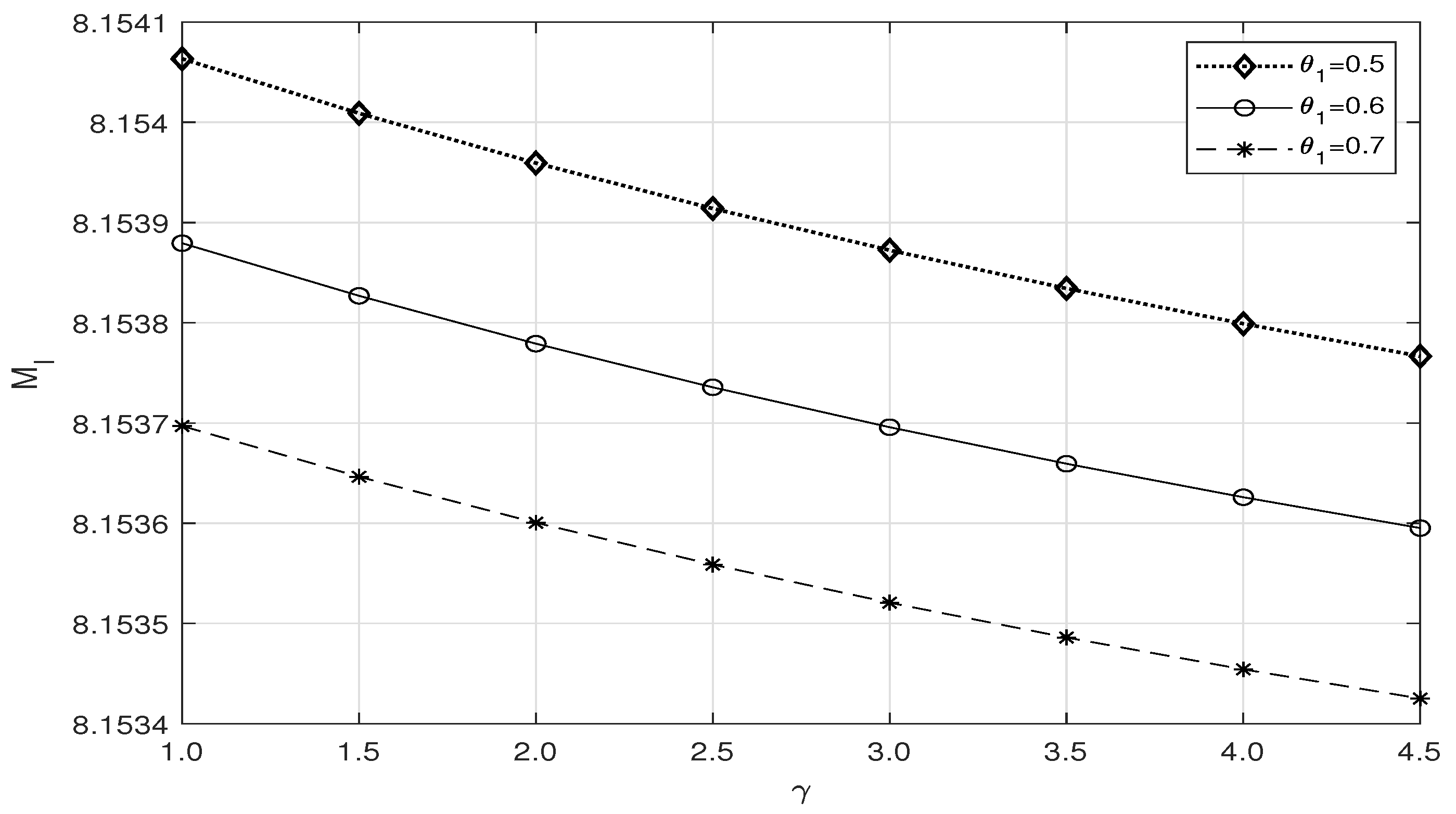
- 1.
- Figure 1 explains the effect of over and γ. Whenever the arrival rate is increased, is increased. The decreases as the vacation completion rate is increased.
- 2.
- The impact of and μ over the average number of customers can be seen in Figure 2. increases as usually the arrival rate is increased. While increasing the service rate, the mean service time decreases, such that the decreases.
- 3.
- The result of varying and γ over the is shown in Figure Table 2. When the retrial rate is increased, decreases. As we know, while increasing the vacation completion rate, the decreases due to the decrease in average time of vacation.
- 4.
- One can identify the result of under the variation of and β from Figure 4. The decreases when we increase the retrial rate. Increasing the reorder rate decreases the mean reorder time. So, the customer in the orbit deceases. Thus, the average number of customers in the orbit decreases while we increase both parameters.
- 5.
- 6.
- The effect of varying the parameters and γ on is shown in Figure 12. If we increase the value of , the number of customer increases in the waiting hall. The vacation period decreases whenever the vacation completion rate is increased. This effect decreases the .
- 7.
- Figure 13 explains the average number of customers present in the waiting hall over the impact of increasing and μ. Due to the increase in arrivals, customers’ arrivals increase in the waiting hall. The mean service time per customer always increases as the service rate increases. So the number of customers available in the waiting hall increases.
- 8.
- The parametric variation of and γ over the is plotted in Figure 14. As we discussed earlier, increases due to the increase in retrial rate. Increasing the parameter γ ensures the availability of the server as the vacation time decreases. So the average number of customers present in the waiting hall decreases.


6. Conclusions
6.1. Observations
- 1.
- The expected total cost analysis explores and verifies the characteristics of the assumed parameters of this model.
- 2.
- The average waiting time of a customer in the waiting hall and orbit are investigated using all the parameters. The monotonicity of the parameters is verified with its characteristics by the numerical simulation.
- 3.
- The discussion of the fraction of time that the server is on vacation suggests that as the server’s vacation duration reduces, his/her fraction time also reduces.
- 4.
- The mean number of customers in the waiting hall and orbit is reduced whenever the average service time per customer and average replenishment time are reduced.
- 5.
- The fraction of the successful rate of retrial is investigated for all the parameters. It helps us to study the retrial customers with different parameter combinations.
6.2. Limitations
6.3. Managerial Implications
Author Contributions
Funding
Institutional Review Board Statement
Informed Consent Statement
Data Availability Statement
Acknowledgments
Conflicts of Interest
References
- Melikov, A.Z.; Molchanov, A.A. Stock optimization in transport/storage. Cybern. Syst. Anal. 1992, 28, 484–487. [Google Scholar] [CrossRef]
- Sigman, K.; Simchi-Levi, D. Light traffic heuristic for an M/G/1 queue with limited inventory. Ann. Oper. Res. 1992, 40, 371–380. [Google Scholar] [CrossRef]
- Berman, O.; Kaplan, E.H.; Shimshak, D.G. Deterministic Approximations for Inventory Management at Service Facilities. IIE Trans. 1993, 25, 98–104. [Google Scholar] [CrossRef]
- Maqbali, K.A.K.A.L.; Joshua, V.C.; Krishnamoorthy, A. On a single server queueing inventory system. In Proceedings of the International Conference on Distributed Computer and Communication Networks, Moscow, Russia, 14–18 September 2020; pp. 579–588. [Google Scholar]
- Mathew, N.; Joshua, V.C.; Krishnamoorthy, A. A Queueing Inventory System with Two Channels of Service. In Proceedings of the International Conference on Distributed Computer and Communication Networks, Moscow, Russia, 14–18 September 2020; pp. 604–616. [Google Scholar]
- Jeganathan, K.; Selvakumar, S.; Saravanan, S.; Anbazhagan, N.; Amutha, S.; Cho, W.; Joshi, G.P.; Ryoo, J. Performance of Stochastic Inventory System with a Fresh Item, Returned Item, Refurbished Item, and Multi-Class Customers. Mathematics 2022, 10, 1137. [Google Scholar] [CrossRef]
- Krishnamoorthy, A.; Nair, S.S.; Narayanan, V.C. An inventory model with server interruptions. In Proceedings of the 5th International Conference on Queueing Theory and Network Applications, Beijing, China, 24–26 July 2010; pp. 132–139. [Google Scholar]
- Krishnamoorthy, A.; Manikandan, R.; Lakshmy, B. A revisit to queueing-inventory system with positive service time. Ann. Oper. Res. 2015, 233, 221–236. [Google Scholar] [CrossRef]
- Jeganathan, K.; Harikrishnan, T.; Selvakumar, S.; Anbazhagan, N.; Amutha, S.; Acharya, S.; Dhakal, R.; Joshi, G.P. Analysis of Interconnected Arrivals on Queueing-Inventory System with Two Multi-Server Service Channels and One Retrial Facility. Electronics 2021, 10, 576. [Google Scholar] [CrossRef]
- Gupta, S.K. Queues with hyper-Poisson input and exponential service time distribution with state dependent arrival and service rates. Oper. Res. 1967, 15, 847–856. [Google Scholar] [CrossRef]
- Boxma, O.; Kaspi, H.; Kella, O.; Perry, D. On/off storage systems with state-dependent input, output, and switching rates. Probab. Eng. Inf. Sci. 2005, 19, 1–14. [Google Scholar] [CrossRef]
- Singh, C.J.; Jain, M.; Kumar, B. Analysis of M/G/1 queueing model with state dependent arrival and vacation. J. Ind. Eng. Int. 2012, 8, 1–8. [Google Scholar] [CrossRef]
- Jeganathan, K.; Reiyas, M.A.; Selvakumar, S.; Anbazhagan, N. Analysis of Retrial Queueing-Inventory System with Stock Dependent Demand Rate:(s,S) Versus (s,Q) Ordering Policies. Int. J. Appl. Comput. Math. 2020, 6, 98. [Google Scholar] [CrossRef]
- Abdul Reiyas, M.; Jeganathan, K. Modeling of Stochastic Arrivals Depending on Base Stock Inventory System with a Retrial Queue. Int. J. Appl. Comput. Math. 2021, 7, 200. [Google Scholar] [CrossRef]
- Nazarov, A.; Dudin, A.; Moiseev, A. Pseudo Steady-State Period in Non-Stationary Infinite-Server Queue with State Dependent Arrival Intensity. Mathematics 2022, 10, 2661. [Google Scholar] [CrossRef]
- Legros, B. Dimensioning a queue with state-dependent arrival rates. Comput. Oper. Res. 2021, 128, 105179. [Google Scholar] [CrossRef]
- Choudhury, G.; Goswami, A.; Begum, A.; Sarmah, H.K. Stochastic Decomposition Results for Poisson Input Queue and Its Applications. Thail. Stat. 2022, 20, 185–194. [Google Scholar]
- Dudin, A.; Dudina, O.; Dudin, S.; Gaidamaka, Y. Self-Service System with Rating Dependent Arrivals. Mathematics 2022, 10, 297. [Google Scholar] [CrossRef]
- Legros, B. The principal-agent problem for service rate event-dependency. Eur. J. Oper. Res. 2022, 297, 949–963. [Google Scholar] [CrossRef]
- Olsson, F. Simple modeling techniques for base-stock inventory systems with state dependent demand rates. Math. Methods Oper. Res. 2019, 90, 61–76. [Google Scholar] [CrossRef]
- Artalejo, J.R.; Krishnamoorthy, A.; Lopez-Herrero, M.J. Numerical analysis of (s, S) inventory systems with repeated attempts. Ann. Oper. Res. 2006, 141, 67–83. [Google Scholar] [CrossRef]
- Manuel, P.; Sivakumar, B.; Arivarignan, G. Perishable inventory system with postponed demands and negative customers. J. Appl. Math. Decis. Sci. 2007, 2007, 94850. [Google Scholar] [CrossRef]
- Ushakumari, P.V. On (s; S ) inventory system with random lead time and repeated demands. J. Appl. Math. Stoch. Anal. 2006, 2006, 81508. [Google Scholar] [CrossRef]
- Jeganathan, K.; Vidhya, S.; Hemavathy, R.; Anbazhagan, N.; Joshi, G.P.; Kang, C.; Seo, C. Analysis of M/M/1/N Stochastic Queueing—Inventory System with Discretionary Priority Service and Retrial Facility. Sustainability 2022, 14, 6370. [Google Scholar] [CrossRef]
- Nithya, M.; Sugapriya, C.; Selvakumar, S.; Jeganathan, K.; Harikrishnan, T. A Markovian two commodity queueing-inventory system with compliment item and classical retrial facility. Ural Math. J. 2022, 8, 90–116. [Google Scholar] [CrossRef]
- Daniel, J.K.; Ramanarayanan, R. An inventory system with two servers and rest periods. In Cahiers du C.E.R.O Bruxelles; University Libre De Bruxelles: Brussels, Belgium, 1987; Volume 29, pp. 95–100. [Google Scholar]
- Daniel, J.K.; Ramanarayanan, R. An (s,S) inventory system with rest periods to the server. In Naval Research Logistics; John Wiley and Sons: Hoboken, NJ, USA, 1988; Volume 35, pp. 119–123. [Google Scholar]
- Zhang, Y.; Yue, D.; Yue, W. A queueing-inventory system with random order size policy and server vacations. Ann. Oper. Res. 2020, 310, 595–620. [Google Scholar] [CrossRef]
- Yue, D.; Qin, Y. A Production Inventory System with Service Time and Production Vacations. J. Syst. Sci. Syst. Eng. 2019, 28, 168–180. [Google Scholar] [CrossRef]
- Koroliuk, V.S.; Melikov, A.Z.; Ponomarenko, L.A.; Rustamov, A.M. Models of Perishable Queueing Inventory Systems with Server Vacation. Cybern. Syst. Anal. 2018, 54, 31–44. [Google Scholar] [CrossRef]
- Yadavalli, V.S.S.; Jeganathan, K. Perishable Inventory Model with Two Heterogeneous Servers Including One with Multiple Vacations and Retrial Customers. J. Control. Syst. Eng. 2015, 3, 10–34. [Google Scholar] [CrossRef]
- Jeganathan, K.; Reiyas, M.A.; Lakshmi, K.P.; Saravanan, S. Two Server Markovian Inventory Systems with Server Interruptions: Heterogeneous Vs. Homogeneous Servers. Math. Comput. Simul. 2019, 155, 177–200. [Google Scholar] [CrossRef]
- Narayanan, V.C.; Deepak, T.G.; Krishnamoorthy, A.; Krishnakumar, B. On an (s,S) inventory policy with service time, vacation to server and correlated lead time. Qual. Technol. Quant. Manag. 2008, 5, 129–143. [Google Scholar] [CrossRef]
- Kathiresan, J.; Jeganathan, K.; Anbazhagan, N. A retrial queueing-inventory system with service option on arrival and Multiple vacations. Afr. Stat. 2019, 14, 1917–1936. [Google Scholar] [CrossRef]
- Revathi, C.; Francis Raj, L. Search of arrivals of an M/G/1 retrial queueing system with delayed repair and optional re-service using modified bernoulli vacation. J. Comput. Math. 2022, 6, 200–209. [Google Scholar]
- Sugapriya, C.; Nithya, M.; Jeganathan, K.; Anbazhagan, N.; Joshi, G.P.; Yang, E.; Seo, S. Analysis of Stock-Dependent Arrival Process in a Retrial Stochastic Inventory System with Server Vacation. Processes 2022, 10, 176. [Google Scholar] [CrossRef]
- Sivakumar, B. An inventory system with retrial demands and multiple server vacation. Qual. Technol. Quant. Manag. 2011, 8, 125–146. [Google Scholar] [CrossRef]
- Manikandan, R.; Sanjeev, S. Nair, M/M/1/1 Queueing-Inventory System with Retrial of Unsatisfied Customers. Commun. Appl. Anal. 2017, 21, 217–236. [Google Scholar]
- Jeganathan, K.; Selvakumar, S.; Anbazhagan, N.; Amutha, S.; Hammachukiattikul, P. Stochastic Modeling on M/M/1/N Inventory System with Queue Dependent Service Rate and Retrial Facility. AIMS Math. 2021, 6, 7386–7420. [Google Scholar] [CrossRef]
- Jeganathan, K.; Reiyas, M.A.; Selvakumar, S.; Anbazhagan, N.; Amutha, S.; Joshi, G.P.; Jeon, D.; Seo, C. Markovian Demands on Two Commodity Inventory System with Queue-Dependent Services and an Optional Retrial Facility. Mathematics 2022, 10, 2046. [Google Scholar] [CrossRef]
- Radhamani, V.; Sivakumar, B.; Arivarignan, G. A Comparative Study on Replenishment Policies for Perishable Inventory System with Service Facility and Multiple Server Vacation. OPSEARCH 2022, 59, 229–265. [Google Scholar] [CrossRef]
- Gupta, P.; Gupta, R.; Malik, S. Impatient Customers in Queueing System with Optional Vacation Policies and Power Saving Mode. Appl. Appl. Math. 2022, 17, 1–17. [Google Scholar]
- Zhang, Y.; Yue, D.; Sun, L.; Zuo, J. Analysis of the Queueing-Inventory System with Impatient Customers and Mixed Sales. Discret. Dyn. Nat. Soc. 2022, 2022, 2333965. [Google Scholar] [CrossRef]
- Krishnamoorthy, A.; Joshua, A.N.; Kozyrev, D. Analysis of a Batch Arrival, Batch Service Queuing-Inventory System with Processing of Inventory While on Vacation. Mathematics 2021, 9, 419. [Google Scholar] [CrossRef]
- Soujanya, M.L.; Laxmi, P.V.; Sirisha, E. Impact of Negative Arrivals and Multiple Working Vacation on Dual Supplier Inventory Model with Finite Lifetimes. Reliab. Theory Appl. 2021, 16, 124–132. [Google Scholar]
- Bouchentouf, A.A.; Cherfaoui, M.; Boualem, M. Analysis and performance evaluation of Markovian feedback multi-server queueing model with vacation and impatience. Am. J. Math. Manag. Sci. 2021, 40, 261–282. [Google Scholar] [CrossRef]
- Beena, P.; Jose, K.P. A MAP/PH (1), PH (2)/2 inventory system with production, multiple servers and vacations. J. Phys. Conf. Ser. 2021, 1850, 012051. [Google Scholar] [CrossRef]
- Ayyappan, G.; Gurulakshmi, G.A.; Somasundaram, B. Analysis of MAP/PH/1 Queueing model with Multiple Vacations, Optional Service, Close-down, Setup, Breakdown, Phase Type Repair and Impatient Customers. Reliab. Theory Appl. 2022, 17, 447–468. [Google Scholar]
- Manikandan, R.; Nair, S.S. An M/M/1 queueing-inventory system with working vacations, vacation interruptions and lost sales. Autom. Remote. Control 2020, 81, 746–759. [Google Scholar] [CrossRef]
- Qu, S.; Li, Y.; Ji, Y. The mixed integer robust maximum expert consensus models for large-scale GDM under uncertainty circumstances. Appl. Soft Comput. 2021, 107, 107369. [Google Scholar] [CrossRef]
- Ji, Y.; Li, H.; Zhang, H. Risk-averse two-stage stochastic minimum cost consensus models with asymmetric adjustment cost. Group Decis. Negot. 2022, 31, 261–291. [Google Scholar] [CrossRef]
- Neuts, M.F. Matrix-Geometric Solutions in Stochastic Models—An Algorithmic Approach; Dover Publication Inc.: New York, NY, USA, 1981. [Google Scholar]
Publisher’s Note: MDPI stays neutral with regard to jurisdictional claims in published maps and institutional affiliations. |
© 2022 by the authors. Licensee MDPI, Basel, Switzerland. This article is an open access article distributed under the terms and conditions of the Creative Commons Attribution (CC BY) license (https://creativecommons.org/licenses/by/4.0/).
Share and Cite
Nithya, M.; Joshi, G.P.; Sugapriya, C.; Selvakumar, S.; Anbazhagan, N.; Yang, E.; Doo, I.C. Analysis of Stochastic State-Dependent Arrivals in a Queueing-Inventory System with Multiple Server Vacation and Retrial Facility. Mathematics 2022, 10, 3041. https://doi.org/10.3390/math10173041
Nithya M, Joshi GP, Sugapriya C, Selvakumar S, Anbazhagan N, Yang E, Doo IC. Analysis of Stochastic State-Dependent Arrivals in a Queueing-Inventory System with Multiple Server Vacation and Retrial Facility. Mathematics. 2022; 10(17):3041. https://doi.org/10.3390/math10173041
Chicago/Turabian StyleNithya, M., Gyanendra Prasad Joshi, C. Sugapriya, S. Selvakumar, N. Anbazhagan, Eunmok Yang, and Ill Chul Doo. 2022. "Analysis of Stochastic State-Dependent Arrivals in a Queueing-Inventory System with Multiple Server Vacation and Retrial Facility" Mathematics 10, no. 17: 3041. https://doi.org/10.3390/math10173041