Efficient Ontology Meta-Matching Based on Interpolation Model Assisted Evolutionary Algorithm

Abstract

Ontology is the kernel technique of the Semantic Web (SW), which models the domain knowledge in a formal and machine-understandable way. To ensure different ontologies’ communications, the cutting-edge technology is to determine the heterogeneous entity mappings through the ontology matching process. During this procedure, it is of utmost importance to integrate different similarity measures to distinguish heterogeneous entity correspondence. The way to find the most appropriate aggregating weights to enhance the ontology alignment’s quality is called ontology meta-matching problem, and recently, Evolutionary Algorithm (EA) has become a great methodology of addressing it. Classic EA-based meta-matching technique evaluates each individual through traversing the reference alignment, which increases the computational complexity and the algorithm’s running time. For overcoming this drawback, an Interpolation Model assisted EA (EA-IM) is proposed, which introduces the IM to predict the fitness value of each newly generated individual. In particular, we first divide the feasible region into several uniform sub-regions using lattice design method, and then precisely evaluate the Interpolating Individuals (INIDs). On this basis, an IM is constructed for each new individual to forecast its fitness value, with the help of its neighborhood. For testing EA-IM’s performance, we use the Ontology Alignment Evaluation Initiative (OAEI) Benchmark in the experiment and the final results show that EA-IM is capable of improving EA’s searching efficiency without sacrificing the solution’s quality, and the alignment’s f-measure values of EA-IM are better than OAEI’s participants.

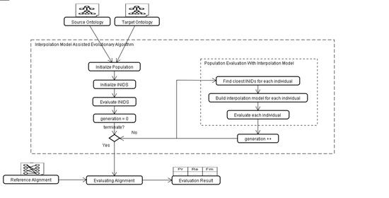
1. Introduction

As the kernel technique of Semantic Web (SW) [1], ontology plays an increasingly key role in such domains as information integration [2], data warehouse [3], e-commerce [4] and knowledge acquisition [5]. According to Bekelman et al. [6], an ontology usually contains the following elements: class or conception: describes the objects collection that are common in a specific province from an abstract perspective. For example, “book” can be represented as a class of all book objects in a bookstore; property or relation: explains the relationships of two entities in a particular province; individual or instance: describes the specific objects that correspond to concepts in the real world; function: the descriptions on a specialized relationship, which links the class to its parent class or an instance; axiom: the descriptions on the theorem that are always true in a particular domain. Figure 1 shows an example of a medical ontology of COVID-19, where the rectangle represents class, one-way arrow between the rectangles denotes the relationship or property, e.g., “coronaviruses” is a subclass of RNA viruses. The instance is represented with circular ova, e.g., “glucocorticoids” is an instance of the medicine.

Although an ontology plays an significant role in the area of knowledge engineering, because of human subjectivity, different ontologies exist the problem of semantic heterogeneity [7], e.g., two ontologies might develop with different OWL languages. Ontology heterogeneity issue greatly affects the communications among different ontologies and the co-operations of their intelligent applications. To achieve the final purpose of SW, it is critical to determine the correspondences between heterogeneous entities, i.e., matching ontologies [8]. Figure 2 illustrates the process of matching two heterogeneous ontologies, where $O_1$ and $O_2$, respectively, denote two ontologies, A and $A^{\prime }$ are, respectively, the final alignment and a partial alignment that could be determined by other ontology matchers, p is a parameter set for the matching process, and r is an external resource set. On this basis, we can formally define the ontology matching process as a function f, which takes as input $O_1$, $O_2$, $A^{\prime }$, p and r, and outputs A.

Since the rapid growth of the ontology, an ontology might own thousands or even more entities, and their semantic relationships become more and more complicated [9], then the ontology matching process gets very complicated. In the ontology matching process, how to measure the similarity of two entities to distinguish the accurate matching elements is a key step in the ontology matching process, which is usually addressed by similarity measures. Similarity measures calculate to the degree of similarity of two entities, which can be divided into two broad categories, which, respectively, based on two entities’ syntax information and linguistic information. Different similarity measures have their own advantages and disadvantages and the applicable scope. Since using only one similarity measure is not enough to obtain satisfying ontology matching results, it is required to integrate multiple measures to enhance the result’s confidence. Ontology meta-matching investigates how to find the optimal integrating weights for similarity measures to improve the ontology alignment’s quality [10], which is a open challenge due to the complex heterogeneous context on entities and the high computational complexity on the matching process [11]. Due to the following two characteristics: (1) the potential parallel search mechanism enables EA to effective explore all the feasible regions; (2) the strong exploration helps prevent the algorithm from falling into the local optimum, and converge to the global optimum, Evolutionary Algorithm (EA) becomes a popular methodology for addressing ontology meta-matching problem [12,13,14].

With respect to the EA-based ontology meta-matching technique, the population’s evaluation is critical for its performance. However, the expensive evaluation, i.e., the evaluation on an individual requires large computational resources, would deteriorate the algorithm’s performance. In the empirical experiment, the classic EA might take about 30 s to evaluate an individual fitness. To improve the algorithm’s efficiency, this work proposes an Interpolation Model assisted EA, which is able to forecast the newly generated individual’s fitness value with a problem-specific IM to save the running time. In particular, we first used the lattice design method [15] to divide the feasible region into several uniform sub-regions and evaluated the representative solutions. After determining which region the newly generated individual was in, an IM was built by using its neighborhood to calculate the fitness value. In particular, the contributions made in this work are as follows:

• a mathematical optimization model on EA-IM based ontology meta-matching problem is constructed;
• a binomial IM based on lattice design is presented to forecast the fitness of the individuals, which is constructed according to the relationship between ontology alignment’s two evaluation metrics;
• an EA-IM is proposed to efficiently address the ontology meta-matching problem.

The rest of the paper is organized as follows: Section 2 presents the related work of ontology meta-matching; Section 3 shows the definitions on ontology matching and the similarity measures; Section 4 presents the construction of Interpolation Model (IM) and the IM-assisted EA; Section 5 shows the experimental results; Section 6 draws the conclusion.

2. Related Work

Similarity measure determines to what extent two entities is similar, and the combination of multiple similarity measures can enhance the quality of alignment. Ontology meta-matching dedicates to investigate the way to find the integrating weights of similarity measures to enhance the ontology alignment’s quality. EA is an outstanding algorithm to overcome ontology meta-matching problem due to its parallel search mechanism and strong exploration, and in recent years, lots of work about EA-based ontology meta-matching techniques are researched. Next, we will review the techniques of EA-based ontology meta-matching in chronological order.

Naya et al. [16] first introduced EA into the field of ontology meta-matching to enhance ontology alignment’s quality. They investigated how to use EA to aggregate multiple similarity measures to optimize the quality of matching results. Starting from the initial population, each individual represented a particular measures combination, and the algorithm iterated to generate the best measures combination. This work was impressive for the development of ontology meta-matching study. Martinez-Gil et al. [17] also proposed an approach based on EA to address the ontology meta-matching problem, which is Genetics for Ontology Alignments (GOAL). Specifically, GOAL described the feasible domain as parameters that were encoded as a chromosome, so the authors devised a way to translate the decimal numbers into a set of floating-point numbers to an arbitrary range of [0, 1]. The authors then constructed one fitness function to select which individuals in the population were more likely to be retained. The experiment proved that GOAL had better scalability and could optimize the matching process. For effectively optimizing the weight of similarity aggregation without knowing the ontology features, Giovanni et al. [18] proposed Memetic Algorithm (MA) to perform the ontology meta-matching to find the sub-optimal alignments. Specifically, MA brings the local search strategy into EA’s evolutionary process, and improved converging speed while ensuring the quality of the solution. This work had shown that the memetic method was an effective way of improving the classic EA-based meta-matching techniques. On this basis, Giovanni et al. [19] proposed an ontology alignment system based on MA, which adjusted its specific instance parameters adaptively with the FML-based fuzzy adjustment to improve the algorithm’s performance. To match several pairs of ontologies at the same time, and overcome the shortcomings of f-measure, Xue et al. [20] proposed the MatchFmeasure, a rough evaluation index without reference matching, and Uniform Improvement Ratio (UIR), a metric to complement MatchFmeasure. This method was able to align multiple pairs of ontologies simultaneously, and avoided the bias improvements on the solutions. In order to better enhance the efficiency of ontology meta-matching process, the Compact EA (CEA) was proposed and used to optimize the aggregating weights [21]. Experimental results showed that CEA could greatly reduce the running time and increase the efficiency. Later on, Parallel CEA (PCEA) [22] was presented to address the meta-matching problem, which combined the parallel technique and compact encoding mechanism. Comparing with CEA, PCEA could further decrease the execution time and main memory consumption of the tuning process, without sacrificing the quality of alignment. Lv et al. [23] proposed a new meta-matching technology for ontology alignment with grasshopper optimization (GSOOM), which used The Grasshopper Optimization Algorithm (GOA) to find the corresponding relationship between the source ontology and target ontology by optimizing the weight of multiple similarity measures. They modeled the ontology meta-matching problem as an optimization GOA individual fitness problem with two objective functions. More recently, Lv et al. [24] introduced an adaptive selection strategy to overcome the premature convergence, which was able to dynamically adjust the selection pressure of the population by changing individual fitness values.

One of the drawbacks that make the existing EA-based matching techniques unable to widely be used in the practical scenarios is their solving efficiency, i.e., they need long running time to find the final alignment especially when evaluating the population. In this work, to address the issue of expensive evaluation, an EA-IM based ontology meta-matching technique is proposed, which makes use of the problem-specific IM to save the algorithm’s running time. In particular, the lattice design is introduced to divide the feasible regions into several parts, which is able to ensure the the accuracy of the approximate evaluation.

3. Preliminaries

3.1. Ontology, Ontology Alignment and Ontology Matching Process

In this work, ontology is defined as follows:

Definition 1.

An ontology can be seen as a 6-tuple O = (C, P, I, ${\phi }_{CP}$, ${\phi }_{CI}$, ${\phi }_{PI}$) [25], where:

• C is a nonempty set of classes;
• P is a nonempty set of properties;
• I is a nonempty set of instances:
• ${\phi }_{CP}$: $P⟶C\times C$ associates a property $pϵP$ with two classes;
• ${\phi }_{CI}$: $C⟶\varphi \left(I\right)$ associates a class $cϵC$ with a subset of I which represents the instances of the concept c;
• ${\phi }_{PI}$: $P⟶\varphi \left(I^2\right)$ associates a property $pϵP$ with a subset of Cartesian product $I\times I$ which represents the pair of instances related through the property p.

To address the ontology heterogeneity issue, the most common method is executing the ontology matching process to determine ontology alignment, which is defined as follows:

Definition 2.

Given two ontology $O_1$ and $O_2$, an ontology alignment is the set of matched elements, and the matched element can be seen as a 5-tuple (id, $e_1$, $e_2$, confidence, relation), where:

• $id$ is the identifier of the matching element;
• $e_1$ and $e_2$ are entities of ontology $O_1$ and $O_2$, respectively;
• $confidence$ is the confidence value of the matched element (generally in the range [0, 1]);
• $relation$ represents the matching relation between entities $e_1$ and $e_2$, such as equivalence relation or generalization relation.

Definition 3.

The ontology matching process is regarded as a β function [26] $A_O$ = β($O_1$, $O_2$, $A_I$, p, r), where $O_1$ and $O_2$ are the two ontologies to be matched, respectively, $A_I$ is an input alignment, p is a set of parameters, r is a set of resources, $A_O$ is a new alignment between $O_1$ and $O_2$. The output alignment $A_O$ is a set of semantic matchings; they can connect entities belonging to $O_1$ with similar entities belonging to $O_2$. The relationship that exists between two ontology entities can be seen as equivalence(≡).

Figure 3 shows the illustration of two heterogeneous ontologies and their alignment. These two ontologies have descriptions of concepts, properties, and instances. Concepts also have inclusion relationships. In this figure, class is described with the rectangle with rounded corners, e.g., class “Chairman” is a specialization (subclass) of class “Person”; The relation between entities has the relation of equivalence and inclusion, entity correspondence is denoted by the thick arrow that links an entity of $O_1$ with an entity of $O_2$, which is represented with the relationship which will be reflected by the correspondence, e.g., “Author” in $O_1$ is more general than Regular author in $O_2$. The “SubjectArea” in $O_1$ and the “Topic” in $O_2$ are a pair of heterogeneous entities, and they are equivalent. An entity is connected with its attributes by dotted lines, e.g., “has email” is a property of the entity “Human” which is defined on the string field.

3.2. Similarity Measure

When matching two ontologies, only those mappings with high similarity value would be regarded as the correct ones. Therefore, how to measure the similarity of two entities to distinguish the correct entity correspondence is critical for ontology matching process. Similarity measure can be used to evaluate the similarity value of two entities to distinguish the correct matching elements. In the ontology matching domain, since syntax-based similarity measure and linguistic-based similarity measure are frequently used [27], in this work, we select two syntax-based similarity measures, i.e., SMOA [28] and N-Gram [29], and one linguistic-based similarity measure, i.e., Wu and Palmer method [30].

SMOA calculates two string’s similarity by taking into account both their similarities and differences between two strings, which is defined in Equation (1):

$$\begin{array}{c}\hfill SMOA(r_1,r_2)=com(r_1,r_2)-dif(r_1,r_2)+winklerlmpr(r_1,r_2)\end{array}$$

(1)

where $com(r_1,r_2)$ is the commonality between two string $r_1$ and $r_2$, $dif(r_1,r_2)$ is their difference and $winklerlmpr(r_1,r_2)$ is the result’s optimisation using the method introduced by Winkler.

Specifically, $com(r_1,r_2)$ first iteratively obtains the maximum common character substring between the strings $r_1$ and $r_2$ until there is no common character substrings. Whenever a maximum public character substring is found, it will be removed from the original string, and the search continues for the next maximum public character substring. Finally, divide the length of the longest common character substring found by the sum of the lengths of the strings $r_1$ and $r_2$ to get the commonality between them. In particular, their commonality is defined as following:

$$com(r_1,r_2)=\frac{2\times {\sum }_i\left|maxComStrin{g}_i\right|}{\left|r_1\right|+\left|r_2\right|}$$

(2)

where $maxComStrin{g}_i$ is the i-th longest common substring between $r_1$ and $r_2$, $\left|r_1\right|$ and $\left|r_2\right|$ are $r_1$ and $r_2$’s cardinality. $dif(r_1,r_2)$ is determined by the length of the character substring that does not match in the first iteration of $com(r_1,r_2)$, which can be defined as Equation (3):

$$dif(r_1,r_2)=\frac{1}{2}\times \frac{\left|d\left(r_1\right)\right|·\left|d\left(r_2\right)\right|}{p+(1-p)(\left|d\left(r_1\right)\right|+\left|d\left(r_2\right)\right|)-\left|d\left(r_1\right)\right|\left|d\left(r_2\right)\right|}$$

(3)

where $d\left(r_1\right)=\frac{|r_1-maxComStrin{g}_i|}{\left|r_1\right|}$ and $d\left(r_2\right)=\frac{|r_2-maxComStrin{g}_i|}{\left|r_2\right|}$, respectively. p is a parameter used to adjust a different importance to the difference component of the SMOA (typically $p=0.6$). In the next, we show an example of calculating SMOA value between two strings “14522345345667890” and “1234567890”. First, their longest common substring is “67890”, and thus $\left|maxComStrin{g}_i\right|=5$. Then, the number of $\left|r_1\right|$ and $\left|r_2\right|$ are 17 and 10, respectively, and the value of $com(r_1,r_2)$ and $winklerlmpr(r_1,r_2)$ are 0.38 and 0.68, respectively. The number of $\left|d\left(r_1\right)\right|$ is 0.5, and the number of $\left|d\left(r_2\right)\right|$ is 0.71, we can obtain $dif(r_1,r_2)=0.24$ according to Equation (3). Finally, two strings’ SMOA value is 0.82 according to Equation (1).

According to [31], N-gram is also a great syntax-based similarity measure because it is able to analyze the similarity between two strings with fine granularity. Given a string, the N-gram of the string represents the segment of the original word sliced by length N, that is, all the n-length substrings in the string. If you have two strings and take their N-gram, you can define the N-gram distance between them in terms of the number of substrings they have in common. As a similarity measure, N-gram can be defined as Equation (4):

$$N\text{-}gram(r_1,r_2)=\frac{2·comm(r_1,r_2)}{N_{r1}+N_{r2}}$$

(4)

where $r_1$ and $r_2$ are the two strings to be compared, and each of them is divided according to certain rules. In the experiment, we set N to 3 and three letters are divided into groups for segmentation. In addition, $comm(r_1,r_2)$ represents the number of sub-strings that are identical between the $r_1$ and $r_2$ strings. $N_{r1}$ and $N_{r2}$ represent the number of substrings $r_1$ and $r_2$ are segmented, respectively. For example, the word “platform” can be cut into six substrings: “pla”, “lat”, “atf”, “tfo”, “for”, and “orm”. The word “plat” can be cut into two substrings: “pla” and “lat”. The same substrings of $r_1$ and $r_2$ are “pla” and “lat”. When calculate the N-gram similarity between “platform” and “plat”, the number of $r_1$ substrings $N_{r1}$ = 6, the number of $r_2$ substrings $N_{r2}$ = 2, and the number of common substrings $r_1$ and $r_2$ which is $com(r_1,r_2)$ = 2 can be substituted into the Equation (4).

Different from the above two metrics, Wu and Palmer’s method uses WordNet [32] to measure the semantic distance of two words. WordNet is an online English vocabulary retrieval system. As a linguistic ontology and semantic dictionary, WordNet is widely used in natural language processing. Here, the closer two terms are to their common parent in semantic depth in WordNet, the more similar they become. Given two words $r_1$ and $r_2$, their linguistic similarity is calculated as follows:

$$Wup(r_1,r_2)=\frac{2·depth\left(LCA(r_1,r_2)\right)}{depth\left(r_1\right)+depth\left(r_2\right)}$$

(5)

where $LCA(r_1,r_2)$ is the closest common parent concept between $r_1$ and $r_2$, $depth\left(LCA(r_1,r_2)\right)$ represents the depth position of the common parent, $depth\left(r_1\right)$ and $depth\left(r_2\right)$ represent the depth position of $r_1$ and $r_2$ in WordNet dictionary, respectively. The smaller the gap between $depth\left(LCA(r_1,r_2)\right)$ and $depth\left(r_1\right)$ and $depth\left(r_2\right)$, the closer the kinship between common parent $LCA(r_1,r_2)$ and $r_1$ and $r_2$, that is, the closer $r_1$ and $r_2$ are. Figure 4 shows an example. The “Animal” in the figure is located in the first layer of the network, which is the lowest layer. According to the Wup calculation rule, both “Bird” and “Fish” are in the second layer, and the nearest common parent is the “Animal” in the first layer. Therefore, the similarity between “Bird” and “Fish” is 2⁄(2 + 2) = 0.5. The concepts “Sparrow” and “Parrot” are both in the third layer, and their common parent is the "bird" in the second level, so that the similarity between “Sparrow” and “Parrot” is $4⁄(3+3)\approx 0.67$. Such results are consistent with the human perception of the world, that “sparrows” and “parrots” are more similar than “Bird” and “Fish”.

3.3. Similarity Aggregation Strategy

Since the complex heterogeneous characteristics between two ontologies, a single similarity measure is hard to ensure its effectiveness on all matching tasks. Therefore, we need to integrate multiple similarity measures to improve the result’s confidence. The most common strategy of aggregating similarity measures is the weighted sum method [33], which is defined as Equation (6):

$$sim{m}_{agg}(e_i,e_j)=\sum _{k=1}^n{w}_k·sim{m}_k(e_i,e_j),subjectto\sum _{k=1}^n{w}_k=1$$

(6)

where $e_i$, $e_j$ are, respectively, two entities from two different ontologies, and $w_k$ is the aggregating weight for kth similarity measure $sim{m}_k$. For example, assuming there are three similarity measures, whose similarity values on two entities are, respectively, $sim{m}_1=0.75$, $sim{m}_2=0.62$ and $sim{m}_3=0.83$, given the aggregating weight vector $(w_1,w_2,w_3)={(0.2,0.3,0.5)}^T$ where $\sum w_i=1$, and the final similarity value is $\sum w_i\times sim{m}_i=0.2\times 0.75+0.3\times 0.62+0.5\times 0.83=0.75$.

3.4. Ontology Meta-Matching Problem

In the field of ontology matching the quality of the final matching is usually measured by the correctness and completeness of the correspondence found. In particular, precision calculates the fraction of matched alignments which are truly correct, and recall calculates the percentage of correct matches found compared to the total number of existing correct matches [34]. In general, precision and recall are comprehensively trade off through f-measure, which is a weighted summed average of them. In this work, f-measure is used to measure the quality of the ontology alignment’s result [35]. Formally, precision, recall and f-measure are, respectively, defined as following:

$$precision=\frac{\left|R\bigcap A\right|}{\left|A\right|}$$

(7)

$$recall=\frac{\left|R\bigcap A\right|}{\left|R\right|}$$

(8)

$$f-measure=\frac{2·precision·recall}{precision+recall}$$

(9)

where R is the reference alignment and A is the alignment.

Given two ontologies $O_1$ and $O_2$, supposing the best alignment of $O_1$ and $O_2$ is a one-to-one relationship, the more correspondences between $O_1$ and $O_2$, and the similarity of the correspondence is proportional to the quality of the alignment. Therefore, ontology alignment quality measure can be obtained as follows:

$$I\left(A\right)=\alpha \times F\left(A\right)+(1-\alpha )\times \frac{{\sum }_i^{\left|A\right|}{\delta }_i}{\left|A\right|}$$

(10)

where $\left|A\right|$ is the number of correspondences in the alignment A, $F\left(\right)$ is a function that evaluates A’s f-measure, ${\delta }_i$ represents the ith correspondence’s similarity value in A and ${\delta }_i$ is a tuning parameter which trades off the ontology alignments characterized by high precision or high recall. Based on the previous work [36], we set ${\delta }_i$ to 0.2. Therefore, we can define the ontology meta-matching problem as follows:

$$\left\{\begin{array}{cc}\hfill & maxI\left(X\right)\hfill \\ \hfill & s.t.X={(x_1,x_2,\cdots ,x_n)}_{}^T,\hfill \\ \hfill & \sum _{i=1}^n{x}_i=1,x_i\in [0,1],i=1,2,\cdots ,n\hfill \end{array}\right.$$

(11)

where the decision variable X is the parameter set, e.g., the weights for aggregating multiple similarity measures and the threshold for filtering the aggregated alignment.

4. Evolutionary Algorithm with Interpolation Model

When evaluating an individual, the traditional way needs to traverse all the correspondences in the reference alignment, which requires long running time. To address this issue, an interpolation model is proposed, which is able to significantly save the running time of EA. The framework of EA-IM based ontology meta-matching is shown in Figure 5:

Before initializing the population, lattice design is used to divide the feasible domain, and 16 standard individuals, i.e., INIDs, are set for calculating individual fitness. In the process of population fitness evaluation, the three INIDs that are most similar to individuals (that is, the closest distance) are firstly found, and interpolation prediction model is constructed by using these three INIDs, then the fitness of individuals is obtained. After that, the individuals are updated by the selection, crossover and mutation operations of the evolutionary algorithm. The algorithm iterates until the maximum number of times, and finally outputs the individuals representing the optimal solution. The following introduction will focus on the coding mechanism of the algorithm, lattice design for feasible domain, EA-IM based ontology matching and evolution operators.

4.1. Encoding Mechanism

The individuals in this article are binary coded, and since three measures are aggregated in this article, each individual contains three similarity values, as well as a threshold for filtering lower similarity values, which are updated with iteration. The encoding scheme in this paper represents weights by defining segmentation points in the interval [0, 1]. Presuming p is the required amount of weights, then set of segmentation points will be obtained as $s^{\prime }$ = {$s_1^{\prime }$, $s_2^{\prime }$, …, $s_{p-1}^{\prime }$}. An individual decoding process is to first select the elements in $S^{\prime }$ in ascending order to get s = {$s_1$, $s_2$, …, $s_{p-1}$}, and then, the corresponding weights are calculated by the following formula:

$$w_k=\left\{\begin{array}{c}\hfill s_1,k=1\\ \hfill s_k-s_{k-1},& 1<k<p\hfill \\ \hfill 1-s_{p-1}\end{array}\right.$$

(12)

Since $p-1$ bits are needed to indicate the split point and 1 bit to indicate the threshold, P represents the length of individual codes. Figure 6 shows an instance of weight encoding and decoding in which there are 6 weights used to integrate 6 different similarity measures:

Then, according to the five segmentation points, the decoded weights are $w_1=s_1-0=0.175$, $w_2=s_2-s_1=0.166$, $w_3=s_3-s_2=0.124$, $w_4=s_4-s_3=0.301$, $w_5=s_5-s_4=0.166$, $w_6=1-s_5=0.068$.

4.2. Binomial Interpolation Model Based on Lattice Design

Due to the large searching space, it is hard to predict the position of a new individual in the feasible region, and thus the most effective method is to uniformly divide the feasible region into several grids in advance. In this work, the crossing points of the grids are called Interpolating Individuals (INIDs), which are precisely evaluated. On this basis, we built IM for evaluating the new individual’s fitness through its nearest INIDs. In particular, we use the simple lattice design [37] to divide the feasible region to ensure the uniform distribution of precisely evaluated individuals, which can accommodate more test processing and theoretically can have a good control of the error of the test.

With respect to the setting of the number of INID, we need to weigh that the efficiency and effectiveness of the algorithm. In this work, since the dimension of the feasible region is 4, the total number of INID is exponentially related to the number of cut points in each dimension. For example, if there are x cut points in each dimension, the total number of INIDs is $x^4$. It is obvious that one cut point will cause large deviation of individual fitness, while three points would produce $3^4=81$ INIDs, which would reduce the efficiency of our algorithm. To better trade off the efficiency and effectiveness, we empirically set cut point of each dimension as two. Therefore, we can get $2^4=16$ INIDs. In addition, regarding the configuration of two cutting points on each dimension, since we need to ensure the uniform distribution of INIDs to the maximum extent, the optimal positions of two points are set as those closest to 1/3 and 2/3 in the interval [0, 1], respectively. In the experiment, we set the two cutting points as 0.33 and 0.66, respectively.

A simple example of dividing two dimensional region is shown in Figure 7 and nine divided regions are marked with numbers from 1 to 9.

After that, given a new individual $ind$, we first construct a plane rectangular coordinate system recall as the horizontal axis and precision the vertical axis, and find its three nearest INIDs $INI{D}_1$, $INI{D}_2$ and $INI{D}_3$, where $INI{D}_1<INI{D}_2<INI{D}_3$ in terms of their distances to $ind$. The distances between $ind$ and $INI{D}_1$ and $INI{D}_2$ are $d1$ and $d2$, respectively. Finally, $ind$’s recall $recal{l}_{predict}\left(ind\right)$ and precision $recal{l}_{predict}$ are calculated according to the following formulas:

$$recal{l}_{predict}=\frac{d_1\times INI{D}_2^{recall}+d_2\times INI{D}_1^{recall}}{d1+d2}$$

(13)

$$precisio{n}_{predict}=a\times recal{l}_{predict}^2+b\times recal{l}_{predict}+c$$

(14)

where $INI{D}_1^{recall}$ and $INI{D}_2^{recall}$ are recall values of $INI{D}_1$ and $INI{D}_2$, respectively, and $a<0$, $b>0$, $c>0$ are the coefficients of a quadratic function determined by $INI{D}_1$, $INI{D}_2$, and $INI{D}_3$.

An example of evaluating a new individual A with IM is shown in Figure 8. In the figure, $X_1$, $X_2$ and $X_3$ are, respectively, three INIDs closest to A, which can be used to construct IM in the form of a quadratic function, $d_1$ ($d_2$) is the distance between A and $X_1$ ($X_2$). In the objective space, $X_1$, $X_2$ and A, respectively, correspond to $X_1^{\prime }$, $X_2^{\prime }$ and $A^{\prime }$, and since $d_1^{\prime }$ and $d_2^{\prime }$, which are, respectively, the distances between $X_1^{\prime }$ and $A^{\prime }$, and $X_2^{\prime }$$A^{\prime }$, are very small, $A^{\prime }$ can be approximately regarded being on IM’s curve. Therefore, the ratio of $d_1$ and $d_2$ is approximately equal to that of $d_1^{\prime }$ and $d_2^{\prime }$, i.e., $\frac{d_1}{d_2}\approx \frac{d_1^{\prime }}{d_2^{\prime }}$. Finally, with this ratio and the coordinate values of $x_1^{\prime }$ and $x_2^{\prime }$, we can determine the coordinate values of $A^{\prime }$ in the objective space through Equations (13) and (14), i.e., $A^{\prime }$’s recall and precision.

The smaller the distance between two individuals, the more similar they are. In this work, we use the Euclidean distance to calculate two individuals’ distance, which is defined in Equation (15):

$$d(p_1,p_2)=\sqrt{{\displaystyle \sum _{i=1}^F}{(p_{1i}-p_{2i})}^2}$$

(15)

where $p_1$ and $p_2$ are two individuals, and F is the number of their features.

4.3. Selection, Crossover and Mutation

Selection aims to select the best individuals in the population by fitness function or other criteria to form the next generation of the population. Selection operation includes roulette selection method, tournament selection method and random traversal sampling method. In order to ensure that excellent individuals have more chances to reproduce, and in consideration of the need to ensure the diversity of the population, the roulette wheel selection method is used, the higher the fitness of the individuals are more likely to be selected.

Crossover refers to the random selection of two individuals from the population, through the exchange of two chromosomes, to produce a new individual to ensure the diversity of the population. In practical application, the single point crossover operator is the most widely used operator, which randomly selects a crossover location in the paired chromosome and then performs gene transposition on the paired chromosome at this crossover location. Using the single point crossover method, the selected individuals are recombined according to a predetermined probability.

Mutation can prevent the EA from falling into the local optimal solution by changing the gene value of some gene loci of some individuals in the population. In practical application, a single point mutation, also known as bit mutation, is mainly used, that is, only one bit in the gene sequence is mutated. Taking binary coding as an example, 0 becomes 1, and 1 becomes 0. We also adopt the method of single point variation.

5. Experiment

5.1. Experimental Configuration

In the experiments, we used the well-known Benchmark provided by Ontology Alignment Evaluation Initiative (OAEI) [38] to test EA-IM’s performance. OAEI is an international ontology Alignment competition designed to evaluate various ontology alignment algorithms for the purpose of evaluating, comparing, communicating and promoting ontology alignment. OAEI’s Benchmark features wide. In particular, it contains 51 ontologies from the same domain, and they are modified manually, some will change natural language tags and comments, etc., while others will replace concepts with random strings. This can fully measure the advantages and inferiority of different ontology matching algorithms. Specifically, these ontologies are divided into three categories, i.e., 1XX, 2XX and 3XX. 1XX (two same ontologies) are those testing cases whose ID begins with 1, whose ontologies are usually used for concept testing, the ontologies of 2XX (two ontologies with different lexical or structure features) are usually used for comparing different modifications, and the ontologies of 3XX (two real world ontologies) are developed by different organizations and come from the same domain in the real world. 16 INIDs of lattice design is shown in

Table 1. 16 INIDs for building interpolation models.

(0.3, 0.3, 0.3, 0.3)	(0.3, 0.3, 0.3, 0.6)
(0.3, 0.3, 0.6, 0.3)	(0.3, 0.3, 0.6, 0.6)
(0.3, 0.6, 0.3, 0.3)	(0.3, 0.6, 0.3, 0.6)
(0.3, 0.6, 0.6, 0.3)	(0.3, 0.6, 0.6, 0.6)
(0.6, 0.3, 0.3, 0.3)	(0.6, 0.3, 0.3, 0.6)
(0.6, 0.3, 0.6, 0.3)	(0.6, 0.3, 0.6, 0.6)
(0.6, 0.6, 0.3, 0.3)	(0.6, 0.6, 0.3, 0.6)
(0.6, 0.6, 0.6, 0.3)	(0.6, 0.6, 0.6, 0.6)

.

First, we compare the matching results and running time of our algorithm with classic EA-based ontology meta-matching to prove that our algorithm greatly improves the efficiency of ontology matching under the condition of having good matching results. Secondly, we compare the matching results of our algorithm with the participants above OAEI, further illustrating the superiority of our matching results. To evaluate our algorithm more comprehensively, the recall, precision and f-measure are used as well as algorithm’s running time to evaluate our method. As mentioned above, recall measures the ratio of all positive examples found in the sample, how many of the samples predicted to be positive by precision are truly positive samples, while f-measure represents the weighted average of recall and precision. Algorithm generation time refers to the time it takes for the algorithm to complete the number of generations we set in advance.

To make the fair comparisons, EA-IM and EA’s parameters are set as the same, which are as follows:

• Population size $PopNum$ = 20,
• Crossover probability $CP$ = 0.6,
• Mutation probability $MP$ = 0.01,
• Maximum generation $MaxGen$ = 1000,

The above configuration follows the following principles:

• Population size. The setting of the population size depends on the complexity of the individual, and according to previous studies [39], population size should be in the range [4$\times n$, 6$\times n$] where n is the decision variable’s dimension number. In this work, the decision variable owns 4 dimensions, so the population size should be in the range [16, 24]. The larger population size is, the longer time population might take to converge. While the smaller it is, the higher probability of which the algorithm suffers from the premature convergence [40]. Since the ontology meta-matching is a small-scale issue, we set the population size as 20.
• Crossover and mutation probability. For crossover and mutation probabilities, small probabilities will decrease the diversity of the population while large probabilities will miss the optimal individuals [41]. Their suggested ranges are, respectively, [0.6, 0.8] and [0.01, 0.05], and since the problem in this work is a low-dimensional problem, we select $CP=0.6$ and $MP=0.01$, whose effectiveness are also verified in the experiment.
• Maximum generation. In EA, the maximum of generations is directly proportional to the scale of the problem [42], and the suggested range is [800, 2000]. Since the ontology meta-matching problem in this work is a 4-dimensional problem, who’s searching region is not very large, the maximum generation should be a relative small value, and in the experiment, $MaxGen=1000$ is robust on all testing cases.

In the experiment, we first compare EA-IM with classic EA-based ontology meta-matching technique in

Table 2. Comparison between EA-IM and EA on OAEI’s Benchmark.

Testing Case	EA-IM	EA-IM	EA-IM	EA	EA	EA
	$\mathit{P}\left(\mathit{stDev}\right)$	$\mathit{R}\left(\mathit{stDev}\right)$	$\mathit{F}\left(\mathit{stDev}\right)$	$\mathit{P}\left(\mathit{stDev}\right)$	$\mathit{R}\left(\mathit{stDev}\right)$	$\mathit{F}\left(\mathit{stDev}\right)$
101	1.000 (0.000)	1.000 (0.024)	1.000 (0.013)	1.000 (0.000)	1.000 (0.000)	1.000 (0.000)
103	1.000 (0.003)	1.000 (0.009)	1.000 (0.006)	1.000 (0.000)	1.000 (0.000)	1.000 (0.000)
104	1.000 (0.000)	1.000 (0.003)	1.000 (0.002)	1.000 (0.000)	1.000 (0.000)	1.000 (0.000)
201	0.989 (0.005)	0.907 (0.007)	0.946 (0.005)	0.989 (0.000)	0.928 (0.000)	0.957 (0.000)
203	1.000 (0.000)	0.979 (0.424)	0.990 (0.390)	1.000 (0.000)	1.000 (0.000)	1.000 (0.000)
204	1.000 (0.000)	0.990 (0.041)	0.995 (0.023)	1.000 (0.000)	1.000 (0.000)	1.000 (0.000)
205	0.974 (0.009)	0.794 (0.014)	0.875 (0.012)	0.989 (0.000)	0.918 (0.004)	0.952 (0.002)
206	1.000 (0.006)	0.876 (0.065)	0.934 (0.041)	1.000 (0.000)	0.928 (0.000)	0.963 (0.000)
207	1.000 (0.009)	0.887 (0.037)	0.940 (0.024)	1.000 (0.000)	0.938 (0.000)	0.968 (0.000)
221	1.000 (0.000)	0.990 (0.005)	0.995 (0.002)	1.000 (0.000)	1.000 (0.000)	1.000 (0.000)
222	1.000 (0.007)	1.000 (0.008)	1.000 (0.007)	1.000 (0.000)	1.000 (0.000)	1.000 (0.000)
223	0.990 (0.005)	0.990 (0.005)	0.990 (0.005)	1.000 (0.000)	0.990 (0.000)	0.995 (0.000)
224	1.000 (0.000)	1.000 (0.024)	1.000 (0.013)	1.000 (0.000)	1.000 (0.000)	1.000 (0.000)
225	1.000 (0.000)	1.000 (0.005)	1.000 (0.003)	1.000 (0.000)	1.000 (0.000)	1.000 (0.000)
228	1.000 (0.014)	1.000 (0.012)	1.000 (0.011)	1.000 (0.000)	1.000 (0.000)	1.000 (0.000)
230	0.935 (0.000)	1.000 (0.000)	0.966 (0.000)	0.986 (0.001)	0.986 (0.000)	0.986 (0.001)
231	1.000 (0.000)	1.000 (0.005)	1.000 (0.002)	1.000 (0.000)	1.000 (0.000)	1.000 (0.000)
232	1.000 (0.000)	1.000 (0.005)	1.000 (0.003)	1.000 (0.000)	1.000 (0.000)	1.000 (0.000)
233	1.000 (0.015)	1.000 (0.015)	1.000 (0.013)	1.000 (0.000)	1.000 (0.000)	1.000 (0.000)
236	1.000 (0.015)	1.000 (0.015)	1.000 (0.015)	1.000 (0.000)	1.000 (0.000)	1.000 (0.000)
237	1.000 (0.000)	1.000 (0.000)	1.000 (0.000)	1.000 (0.001)	1.000 (0.000)	1.000 (0.001)
238	0.990 (0.005)	0.979 (0.005)	0.984 (0.005)	0.990 (0.000)	0.990 (0.000)	0.990 (0.000)
239	1.000 (0.000)	1.000 (0.000)	1.000 (0.000)	1.000 (0.000)	1.000 (0.000)	1.000 (0.000)
240	0.969 (0.000)	0.939 (0.000)	0.954 (0.000)	1.000 (0.009)	0.970 (0.000)	0.985 (0.005)
241	1.000 (0.014)	1.000 (0.014)	1.000 (0.012)	1.000 (0.000)	1.000 (0.000)	1.000 (0.000)
246	1.000 (0.000)	0.966 (0.000)	0.983 (0.000)	1.000 (0.000)	1.000 (0.000)	1.000 (0.000)
247	0.969 (0.000)	0.939 (0.000)	0.954 (0.000)	1.000 (0.009)	0.970 (0.000)	0.985 (0.005)
248	1.000 (0.000)	0.010 (0.000)	0.020 (0.000)	0.500 (0.000)	0.021 (0.000)	0.040 (0.000)
301	0.960 (0.008)	0.814 (0.007)	0.881 (0.006)	0.980 (0.001)	0.814 (0.000)	0.889 (0.001)
302	0.906 (0.012)	0.604 (0.006)	0.725 (0.005)	1.000 (0.000)	0.604 (0.000)	0.753 (0.000)
303	0.884 (0.017)	0.770 (0.029)	0.822 (0.023)	0.870 (0.028)	0.833 (0.020)	0.851 (0.001)
Average	0.986	0.917	0.934	0.978	0.932	0.946

in terms of precision, recall and f-measure and the symbols P, R and F, respectively, represent precision, recall and f-measure. Then, we show the corresponding box-and-whisker plots in Figure 9, Figure 10 and Figure 11. After that, we compare their running time in

Table 3. Comparison of EA-IM and EA in terms of Running Time (millisecond).

Testing Case	EA-IM	EA
101	1459	32,762
103	1346	32,382
104	1448	32,214
201	1639	32,267
203	1899	32,802
204	2116	33,212
205	2130	33,267
206	1995	32,613
207	1784	33,615
221	1552	32,863
222	1623	32,832
223	1663	33,643
224	1479	33,913
225	2103	33,455
228	1721	22,436
230	2071	28,423
231	1951	33,460
232	2066	33,181
233	1738	22,404
236	1328	22,636
237	1735	32,362
238	2323	34,396
239	1708	22,190
240	2005	22,326
241	1830	22,696
246	1905	21,829
247	1818	22,177
248	2149	32,493
301	2031	26,488
302	1869	23,982
303	2125	25,481
Average	1826	29,395

, and finally, we compare EA-IM with OAEI’s participants in terms of f-measure and running time in

Table 4. Comparison among EA-IM and OAEI’s participants in terms of f-measure on Benchmark.

Testing Case	Edna	AgrMaker	AROMA	ASMOV	CODI	Ef2Match	Falcon	GeRMeSMB	MapPSO	RiMOM	SOBOM	TaxoMap	EA-IM
101	1.00	0.99	0.98	1.00	1.00	1.00	1.00	1.00	1.00	1.00	1.00	0.51	1.00
103	1.00	0.99	0.99	1.00	1.00	1.00	1.00	1.00	1.00	1.00	1.00	0.51	1.00
104	1.00	0.99	0.99	1.00	0.99	1.00	1.00	1.00	1.00	1.00	1.00	0.51	1.00
201	0.04	0.92	0.95	1.00	0.13	0.77	0.97	0.94	0.42	1.00	0.95	0.51	0.95
203	1.00	0.98	0.80	1.00	0.86	1.00	1.00	0.98	1.00	1.00	1.00	0.49	0.99
204	0.93	0.97	0.97	1.00	0.74	0.99	0.96	0.98	0.98	1.00	0.99	0.51	0.99
205	0.34	0.92	0.95	0.99	0.28	0.84	0.97	0.99	0.73	0.99	0.96	0.51	0.88
206	0.54	0.93	0.95	0.99	0.39	0.87	0.94	0.92	0.85	0.99	0.96	0.51	0.93
207	0.54	0.93	0.95	0.99	0.42	0.87	0.96	0.96	0.81	0.99	0.96	0.51	0.94
221	1.00	0.97	0.99	1.00	0.98	1.00	1.00	1.00	1.00	1.00	1.00	0.51	0.99
222	0.98	0.98	0.99	1.00	1.00	1.00	1.00	0.99	1.00	1.00	1.00	0.46	1.00
223	1.00	0.95	0.93	1.00	1.00	1.00	1.00	0.96	0.98	0.98	0.99	0.45	0.99
224	1.00	0.99	0.97	1.00	1.00	1.00	0.99	1.00	1.00	1.00	1.00	0.51	1.00
225	1.00	0.99	0.99	1.00	0.99	1.00	1.00	1.00	1.00	1.00	1.00	0.51	1.00
228	1.00	1.00	1.00	1.00	1.00	1.00	1.00	1.00	1.00	1.00	1.00	1.00	1.00
230	0.85	0.90	0.93	0.97	0.98	0.97	0.97	0.94	0.98	0.97	0.97	0.49	0.97
231	1.00	0.99	0.98	1.00	1.00	1.00	1.00	1.00	1.00	1.00	1.00	0.51	1.00
232	1.00	0.97	0.97	1.00	0.97	1.00	0.99	1.00	1.00	1.00	1.00	0.51	1.00
233	1.00	1.00	1.00	1.00	0.94	1.00	1.00	0.98	1.00	1.00	1.00	1.00	1.00
236	1.00	1.00	1.00	1.00	1.00	1.00	1.00	1.00	1.00	1.00	1.00	1.00	1.00
237	0.98	0.98	0.97	1.00	0.99	1.00	0.99	1.00	0.99	1.00	1.00	0.46	1.00
238	1.00	0.94	0.92	1.00	0.99	1.00	0.99	0.96	0.97	0.98	0.98	0.45	0.98
239	0.50	0.98	0.98	0.98	0.98	0.98	1.00	0.98	0.98	0.98	0.98	0.94	1.00
240	0.55	0.91	0.83	0.98	0.95	0.98	1.00	0.85	0.92	0.94	0.98	0.88	0.95
241	1.00	0.98	0.98	1.00	0.94	1.00	1.00	0.98	1.00	1.00	1.00	1.00	1.00
246	0.50	0.98	0.97	0.98	0.98	0.98	1.00	0.98	0.98	0.98	0.95	0.94	0.98
247	0.55	0.88	0.80	0.98	0.98	0.98	1.00	0.91	0.89	0.94	0.98	0.88	0.95
248	0.03	0.72	0.00	0.87	0.00	0.02	0.00	0.37	0.05	0.64	0.48	0.02	0.02
301	0.59	0.59	0.73	0.86	0.38	0.71	0.78	0.71	0.64	0.73	0.84	0.43	0.88
302	0.43	0.32	0.35	0.73	0.59	0.71	0.71	0.41	0.04	0.73	0.74	0.40	0.73
303	0.00	0.78	0.59	0.83	0.65	0.83	0.77	0.00	0.00	0.86	0.50	0.36	0.82
Average	0.75	0.92	0.88	0.97	0.81	0.92	0.94	0.90	0.85	0.96	0.94	0.59	0.93

and

Table 5. Comparison among EA-IM and OAEI’s participants in terms of running time.

Testing Case	Running Time (Second)	F-Measure per Second
AML	120	0.0031
CroMatcher	1100	0.0008
Lily	2211	0.0004
LogMap	194	0.0028
PhenoMF	1632	0.0000
PhenoMM	1743	0.0000
PhenoMP	1833	0.0000
XMap	123	0.0045
LogMapBio	54,439	0.0000
EA	29.395	0.0322
EA-IM	1.826	0.5115

. The results shown in the table and figures are the mean value of 30 independent runs.

5.2. Experimental Results

It can be seen from Table 2 that the mean f-measure of EA-IM and EA are 0.934 and 0.946, respectively. In addition, to further measure their results’ degree of closeness, we calculated their mean difference value. In particular, the mean difference first calculates two method’s absolute value of their difference on each testing cases, and then calculates their mean value. In the experiment, the mean difference value between EA-IM and EA is 0.012, which shows that the results of EA-IM and EA are very close to each other. On testing cases 1XX, the f-measure values of EA-IM are all 1.000, which shows that it is able to effectively find all correct entity pairs under simple heterogeneous context. On testing cases 2XX and 3XX, EA-IM is also able to find high-quality of alignments in terms of both recall and precision. When facing complex heterogeneous ontologies, the utilization of two syntax-based similarity measures and a linguistic-based similarity measure enables it to distinguish heterogeneous entities under different contexts. We need to point out that on testing case 248, EA-IM’s f-measure is relatively low. The ontology have little lexical and linguistic information in this matching task, and it requires the matching technique making use of the context information to find more correspondences. However, EA-IM does not use the context-based similarity measure, which directly affects the quality of alignment on these testing cases. In general, EA-IM’s results are very close to those of EA, and it has a relatively low average standard deviation, which shows that the proposed IM is effective to approximately evaluate the individual’s fitness and is also of help to enhance the algorithm’s stability.

In Figure 9, the upper edge of both methods is 1.000; the lower edge of EA-IM is 0.974, while the lower edge of EA is 1.000, with a difference of 2.6% between the results of the two methods; the median of EA-IM is 1.000, while the median of EA is 1.000. Therefore, it visually illustrates that EA-IM and EA have a high degree of proximity in terms of precision. In Figure 10, the upper edge of both methods is 1.000; the lower edge of EA-IM is 0.770, while the lower edge of EA is 0.918, with a difference of 16.1% between the results of the two methods. This gap is caused by the low results of EA-IM in testing case 248, 302 and 303 because of the more complex lexical information of these ontologies. However, this does not affect the excellent performance of EA-IM in terms of the final result (f-measure); the median of EA-IM is 0.990, while the median of EA is 1.000, with a difference of 1.0%. In Figure 11, the upper edge of both methods is 1.000; the lower edge of EA-IM is 0.875, while the lower edge of EA is 0.952, with a difference of 8.1% between the results of the two methods; the median of EA-IM is 0.995, while the median of EA is 1.000, with a difference of 0.5%. The experimental results shown in these figures further show the effectiveness of IM.

In Table 3, the average running time of EA-IM is 1826 milliseconds, while the average running time of EA is 29,395 milliseconds, and the improvement degree is 93.79%. Regarding classic EA-based matching technique, each individual needs to be evaluated by comparing its corresponding alignment with the reference one, which consumes huge running time. With the introduction of IM, we construct a problem-specific mathematical model to forecast the individual’s fitness value, which will decrease the computational complexity, and therefore decrease the running time. From Table 4, EA-IM’s f-measure values are higher than those of OAEI’s participants, which shows that the iterative refining mechanism can effectively improve the alignment’s quality. From the above results, we can draw the conclusion that EA-IM can efficiently address the ontology meta-matching problem and determine high-quality alignments.

Table 5 shows the comparison among EA-IM and OAEI’s participants in terms of running. In Table 5, the matcher’s f-measure per second is calculated by dividing its average F measure by the average running time, which is a measure used by OAEI to measure matcher efficiency. As can be seen, our algorithm is faster than other matchers, which is because we have introduced IM to EA to improve the efficiency of ontology matching.

6. Conclusions and Future Work

Ontology is a new reference model for information exchange, which can be used to get the most accurate semantic normalization description. However, because of the subjectivity of ontology designers, there exists heterogeneity problem between different ontologies, which greatly hinders their semantic interoperability. To solve this problem, researchers need to find semantically identical entities in two ontologies, which is the so-called ontology matching. For EA-based ontology matching techniques, population’s evaluation is of great importance to affect the performance of the algorithm. However, the traditional way of evaluating an individual requires traversing the reference alignment, which results in high computational cost and reduces the algorithm’s performance. To overcome this drawback, we propose an EA-IM ontology meta-matching technique, which introduces the IM to predict the fitness value of each newly generated individual. In particular, we first divide the feasible region into several uniform sub-regions using lattice design method, and then precisely evaluate INIDs. On this basis, an IM is constructed for each new individual to forecast its fitness value, with the help of its neighborhood. The experimental results show that IM can help EA greatly explore the feasible region and determine high-quality alignments efficiently.

To further improve the performance of EA-IM, we are interested in adaptively adjusting the number of INIDs according to the matching task’s heterogeneity feature. In addition, we are also interested in training the problem-specific similarity measures to better distinguish the heterogeneous entities, which should take into consideration of the entity’s context information. Last but not the least, when the scale of ontologies become large, an efficiency-improving strategy, such as the correspondence pruning strategy, could be introduced to control the scale of each similarity measure’s corresponding similarity matrix, which is helpful to optimize the algorithm’s efficiency.

References

- Guarino, N.; Oberle, D.; Staab, S. What is an ontology? In Handbook on Ontologies; Springer: Berlin/Heidelberg, Germany, 2009; pp. 1–17. [Google Scholar]
- Arens, Y.; Chee, C.Y.; Knoblock, C.A. Retrieving and Integrating Data from Multiple Information Sources. Int. J. Coop. Inf. Syst. 1993, 2, 127–158. [Google Scholar] [CrossRef]
- Baumbach, J.; Brinkrolf, K.; Czaja, L.F.; Rahmann, S.; Tauch, A. CoryneRegNet: An ontology-based data warehouse of corynebacterial transcription factors and regulatory networks. BMC Genom. 2006, 7, 24. [Google Scholar] [CrossRef] [PubMed]
- Wang, X.; Ni, Z.; Cao, H. Research on association rules mining based-on ontology in e-commerce. In Proceedings of the 2007 International Conference on Wireless Communications, Networking and Mobile Computing, Shanghai, China, 21–25 September 2007; pp. 3549–3552. [Google Scholar]
- Tu, S.W.; Eriksson, H.; Gennari, J.H.; Shahar, Y.; Musen, M.A. Ontology-based configuration of problem-solving methods and generation of knowledge-acquisition tools: Application of PROTÉGÉ-II to protocol-based decision support. Artif. Intell. Med. 1995, 7, 257–289. [Google Scholar] [CrossRef]
- Gruber, T.R. A translation approach to portable ontology specifications. Knowl. Acquis. 1993, 5, 199–220. [Google Scholar] [CrossRef]
- Kashyap, V.; Sheth, A. Semantic heterogeneity in global information systems: The role of metadata, context and ontologies. Coop. Inf. Syst. Curr. Trends Dir. 1998, 139, 178. [Google Scholar]
- Doan, A.; Madhavan, J.; Domingos, P.; Halevy, A. Ontology matching: A machine learning approach. In Handbook on Ontologies; Springer: Berlin/Heidelberg, Germany, 2004; pp. 385–403. [Google Scholar]
- Verhoosel, J.P.; Van Bekkum, M.; van Evert, F.K. Ontology matching for big data applications in the smart dairy farming domain. In Proceedings of the OM, Bethlehem, PA, USA, 11–12 October 2015; pp. 55–59. [Google Scholar]
- Martinez-Gil, J.; Aldana-Montes, J.F. An overview of current ontology meta-matching solutions. Knowl. Eng. Rev. 2012, 27, 393–412. [Google Scholar] [CrossRef]
- Xue, X.; Huang, Q. Generative adversarial learning for optimizing ontology alignment. Expert Syst. 2022, e12936. [Google Scholar] [CrossRef]
- Arulkumaran, K.; Cully, A.; Togelius, J. AlphaStar: An Evolutionary Computation Perspective. In Proceedings of the Genetic and Evolutionary Computation Conference Companion, GECCO ’19, Prague, Czech Republic, 13–17 July 2019; Association for Computing Machinery: New York, NY, USA, 2019; pp. 314–315. [Google Scholar] [CrossRef]
- Vikhar, P.A. Evolutionary algorithms: A critical review and its future prospects. In Proceedings of the 2016 International Conference on Global Trends in Signal Processing, Information Computing and Communication (ICGTSPICC), Jalgaon, India, 22–24 December 2016; pp. 261–265. [Google Scholar] [CrossRef]
- Eiben, A.E.; Smith, J.E. What is an evolutionary algorithm? In Introduction to Evolutionary Computing; Springer: Berlin/Heidelberg, Germany, 2015; pp. 25–48. [Google Scholar]
- Jiao, Y.; Xu, G. Optimizing the lattice design of a diffraction-limited storage ring with a rational combination of particle swarm and genetic algorithms. Chin. Phys. C 2017, 41, 027001. [Google Scholar] [CrossRef]
- Naya, J.M.V.; Romero, M.M.; Loureiro, J.P.; Munteanu, C.R.; Sierra, A.P. Improving ontology alignment through genetic algorithms. In Soft Computing Methods for Practical Environment Solutions: Techniques and Studies; IGI Global: New York, NY, USA, 2010; pp. 240–259. [Google Scholar]
- Martinez-Gil, J.; Aldana-Montes, J.F. Evaluation of two heuristic approaches to solve the ontology meta-matching problem. Knowl. Inf. Syst. 2011, 26, 225–247. [Google Scholar] [CrossRef] [Green Version]
- He, H.; Tan, Y. A two-stage genetic algorithm for automatic clustering. Neurocomputing 2012, 81, 49–59. [Google Scholar] [CrossRef]
- Huang, H.D.; Acampora, G.; Loia, V.; Lee, C.S.; Kao, H.Y. Applying FML and fuzzy ontologies to malware behavioural analysis. In Proceedings of the 2011 IEEE International Conference on Fuzzy Systems (FUZZ-IEEE 2011), Taipei, Taiwan, 27–30 June 2011; pp. 2018–2025. [Google Scholar]
- Xue, X.; Wang, Y.; Ren, A. Optimizing ontology alignment through memetic algorithm based on partial reference alignment. Expert Syst. Appl. 2014, 41, 3213–3222. [Google Scholar] [CrossRef]
- Xue, X.; Liu, J.; Tsai, P.W.; Zhan, X.; Ren, A. Optimizing Ontology Alignment by Using Compact Genetic Algorithm. In Proceedings of the 2015 11th International Conference on Computational Intelligence and Security (CIS), Shenzhen, China, 19–20 December 2015; pp. 231–234. [Google Scholar] [CrossRef]
- Xue, X.; Jiang, C. Matching sensor ontologies with multi-context similarity measure and parallel compact differential evolution algorithm. IEEE Sens. J. 2021, 21, 24570–24578. [Google Scholar] [CrossRef]
- Lv, Z.; Peng, R. A novel meta-matching approach for ontology alignment using grasshopper optimization. Knowl.-Based Syst. 2020, 201–202, 106050. [Google Scholar] [CrossRef]
- Lv, Q.; Zhou, X.; Li, H. Optimizing Ontology Alignments Through Evolutionary Algorithm with Adaptive Selection Strategy. In Advances in Intelligent Systems and Computing, Proceedings of the International Conference on Advanced Machine Learning Technologies and Applications, Cairo, Egypt, 20–22 March 2021; Springer: Cham, Switzerland, 2021; pp. 947–954. [Google Scholar]
- Xue, X.; Yao, X. Interactive ontology matching based on partial reference alignment. Appl. Soft Comput. 2018, 72, 355–370. [Google Scholar] [CrossRef]
- Xue, X. Complex ontology alignment for autonomous systems via the Compact Co-Evolutionary Brain Storm Optimization algorithm. ISA Trans. 2022; in press. [Google Scholar] [CrossRef]
- Xue, X.; Pan, J.S. A segment-based approach for large-scale ontology matching. Knowl. Inf. Syst. 2017, 52, 467–484. [Google Scholar] [CrossRef]
- Winkler, W.E. The State of Record Linkage and Current Research Problems; Statistical Research Division, US Census Bureau: Suitland-Silver Hill, MD, USA, 1999.
- Mascardi, V.; Locoro, A.; Rosso, P. Automatic ontology matching via upper ontologies: A systematic evaluation. IEEE Trans. Knowl. Data Eng. 2009, 22, 609–623. [Google Scholar] [CrossRef]
- Wu, Z.; Palmer, M. Verbs semantics and lexical selection. In Proceedings of the 32nd annual meeting on Association for Computational Linguistics (COLING-94), Las Cruces, NM, USA, 27–30 June 1994. [Google Scholar]
- Ferranti, N.; Rosário Furtado Soares, S.S.; de Souza, J.F. Metaheuristics-based ontology meta-matching approaches. Expert Syst. Appl. 2021, 173, 114578. [Google Scholar] [CrossRef]
- Fellbaum, C. WordNet. In Theory and Applications of Ontology: Computer Applications; Springer: Berlin/Heidelberg, Germany, 2010; pp. 231–243. [Google Scholar]
- Golberg, D.E. Genetic algorithms in search, optimization, and machine learning. Addion Wesley 1989, 1989, 36. [Google Scholar]
- Ehrig, M.; Euzenat, J. Relaxed precision and recall for ontology matching. In Proceedings of the K-Cap 2005 Workshop on Integrating Ontology, Banff, AB, Canada, 2 October 2005; pp. 25–32. [Google Scholar]
- Faria, D.; Pesquita, C.; Santos, E.; Palmonari, M.; Cruz, I.F.; Couto, F.M. The agreementmakerlight ontology matching system. In Lecture Notes in Computer Science, Proceedings of the OTM Confederated International Conferences “On the Move to Meaningful Internet Systems”, Graz, Austria, 9–13 September 2013; Springer: Berlin/Heidelberg, Germany, 2013; pp. 527–541. [Google Scholar]
- Acampora, G.; Loia, V.; Vitiello, A. Enhancing ontology alignment through a memetic aggregation of similarity measures. Inf. Sci. 2013, 250, 1–20. [Google Scholar] [CrossRef]
- Yates, F. A new method of arranging variety trials involving a large number of varieties. J. Agric. Sci. 1936, 26, 424–455. [Google Scholar] [CrossRef]
- Achichi, M.; Cheatham, M.; Dragisic, Z.; Euzenat, J.; Faria, D.; Ferrara, A.; Flouris, G.; Fundulaki, I.; Harrow, I.; Ivanova, V.; et al. Results of the ontology alignment evaluation initiative 2016. In Proceedings of the OM: Ontology Matching, Kobe, Japan, 18 October 2016; pp. 73–129. [Google Scholar]
- Liu, X. A research on Population Size Impaction on the Performance of Genetic Algorithm. Ph.D. Thesis, North China Electric Power University, Beijing, China, 2010. [Google Scholar]
- Mirjalili, S. Genetic algorithm. In Evolutionary Algorithms and Neural Networks; Springer: Berlin/Heidelberg, Germany, 2019; pp. 43–55. [Google Scholar]
- Xue, X.; Wang, Y. Using memetic algorithm for instance coreference resolution. IEEE Trans. Knowl. Data Eng. 2015, 28, 580–591. [Google Scholar] [CrossRef]
- Xue, X.; Chen, J. Matching biomedical ontologies through Compact Differential Evolution algorithm with compact adaption schemes on control parameters. Neurocomputing 2021, 458, 526–534. [Google Scholar] [CrossRef]
Figure 1.
An Example of Medical Ontology On COVID-19.
Figure 2.
Ontology matching process.
Figure 3.
An Example of Heterogeneous Ontologies and Ontology Alignment.
Figure 4.
Depth position diagram.
Figure 5.
The framework of EA-IM based ontology meta-matching.
Figure 6.
Weight coding and decoding examples.
Figure 7.
An example of feasible region division.
Figure 8.
The interpolation model.
Figure 9.
Comparison of EA-IM and EA on the Box-and-whisker Plot in terms of precision.
Figure 10.
Comparison of EA-IM and EA on the Box-and-whisker Plot in terms of recall.
Figure 11.
Comparison of EA-IM and EA on the Box-and-whisker Plot in terms of f-measure.