
Diverse Multiple Lump Analytical Solutions for Ion Sound and Langmuir Waves

1
Mathematics Department, College of Science, Jouf University, Sakaka 72341, Saudi Arabia
2
Mathematics Department, Faculty of Science, Taibah University, Al-Madinah Al-Munawarah 41411, Saudi Arabia
3
Department of Mathematics, COMSATS University Islamabad, Lahore Campus, Sakaka 72341, Pakistan
*
Author to whom correspondence should be addressed.
Mathematics 2022, 10(2), 200; https://doi.org/10.3390/math10020200
Submission received: 28 October 2021
/
Revised: 14 December 2021
/
Accepted: 23 December 2021
/
Published: 10 January 2022
(This article belongs to the Special Issue Nonlinear Partial Differential Equations: Exact Solutions, Symmetries, Methods, and Applications)
Abstract
:In this work, we study a time-fractional ion sound and Langmuir waves system (FISLWS) with Atangana–Baleanu derivative (ABD). We use a fractional ABD operator to transform our system into an ODE. We investigate multiwaves, periodic cross-kink, rational, and interaction solutions by the combination of rational, trigonometric, and various bilinear functions. Furthermore, 3D, 2D, and relevant contour plots are presented for the natural evolution of the gained solutions under the selection of proper parameters.
1. Introduction
At the present time, various real phenomena have been formulated by integer-order nonlinear partial differential equations (NPDEs). These supermodels are studied in different domains of sciences, such as engineering, chemistry, biology, physics, optics, etc. However, it is not enough to use integer order where the nonlocal property does not appear in these forms, so different models have been systematized in fractional NPDEs to determine that kind of similarity [1]. By using numerical and computational schemes, these models give more familiar properties [2,3,4,5,6,7,8,9,10]. To use most of these schemes, one needs fractional operator to transform the fractional forms into nonlinear ODEs with integer orders such as conformable fractional derivative, Caputo, Caputo–Fabrizio definition, Riemann–Liouville derivatives, and so on [11,12,13,14,15,16,17,18,19,20,21,22,23,24]. These operators have been applied to estimate the numeric and exact solutions of fractional order NPDEs through different integration schemes, such as -model expansion [25], -expansion [26], -expansion [27], Kudryashove scheme [28], -expansion [29], extended auxiliary equation technique [30], and so many others.
Here, we consider the FISLWS as follows [17],
where and n illustrate the normalized electric-field of the Langmuir oscillation and perturbation of density, respectively. Both x and t are normalized variables and is the AB fractional operator in t direction.
ABD operator is well defined as
where is Mittag-Leffler function, defined as
and is the normalization function that satisfies . Thus,
for more properties of this operator. This leads towards the following form,
where and are arbitrary constants. This wave alteration converts Equation (1) into the following ODE.
Here, u and v are the functions of . By separating the Img part from the first part of Equation (6),
and then by integrating the second part of Equation (6) by two times the w.r.t , we obtain
Equations (7) and (8) transform Equation (6) into the following form:
The contents of this paper are arranged as follows: In Section 2, we present M-shaped rational solitons. In Section 3, we evaluate M-shaped interaction solutions. In Section 4, we find the multiwaves solution. In Section 5, we study homoclinic breather. In Section 6, we investigate periodic cross-kink solutions. In Section 7, we present results and discussions and Section 8 contains concluding remarks.
2. M-Shaped Rational Solitons
By using the following log transformation,
We choose M-shaped rational solution in bilinear form for , as follows [31]:
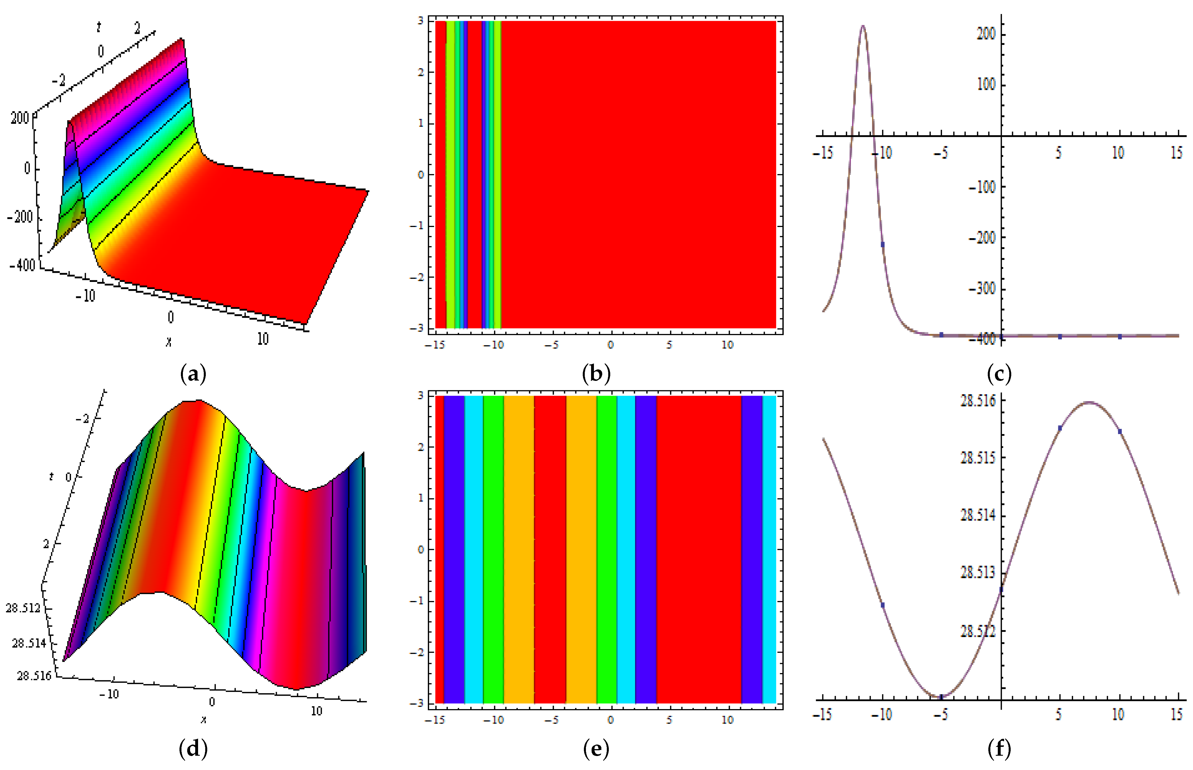
where all are real-valued parameters to be measured. Inserting into Equation (11) and collecting all powers of , we obtain proper results, as follows (See Figure 1 and Figure 2):
Set I. For ,
Using this in Equation (12), and then by using Equations (8) and (10), we obtain
To obtain final results, we use Equation (5):
where .
Set II. For ,
Using this in Equation (12), and then by using Equations (8) and (10) in Equation (5), we obtain
where .
Set III. For ,
Using this in Equation (12), and then by using Equations (8) and (10), we obtain
To obtain final results, we use Equation (5):
where .
3. M-Shaped Rational Soliton Interactions with
In this part, we evaluate M-shaped rational interactions with periodic and kink waves by using exponential and cos function in bilinear combinations.
3.1. One-Kink Soliton
For this, the bilinear form for is as follows [31]:
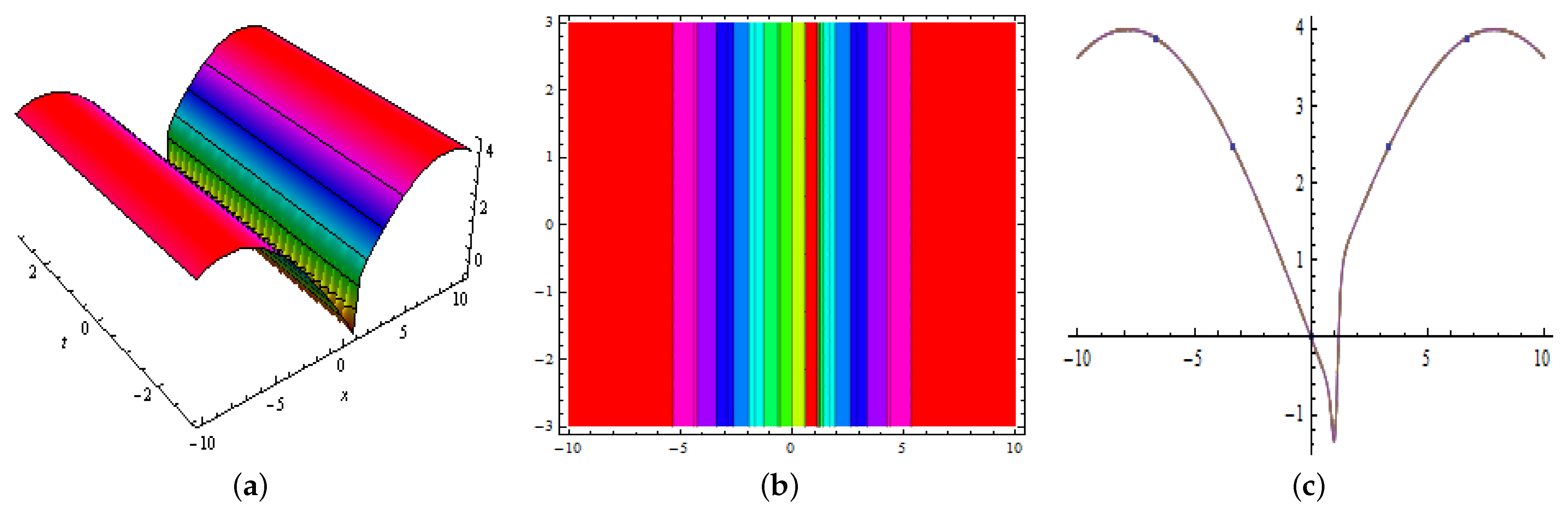
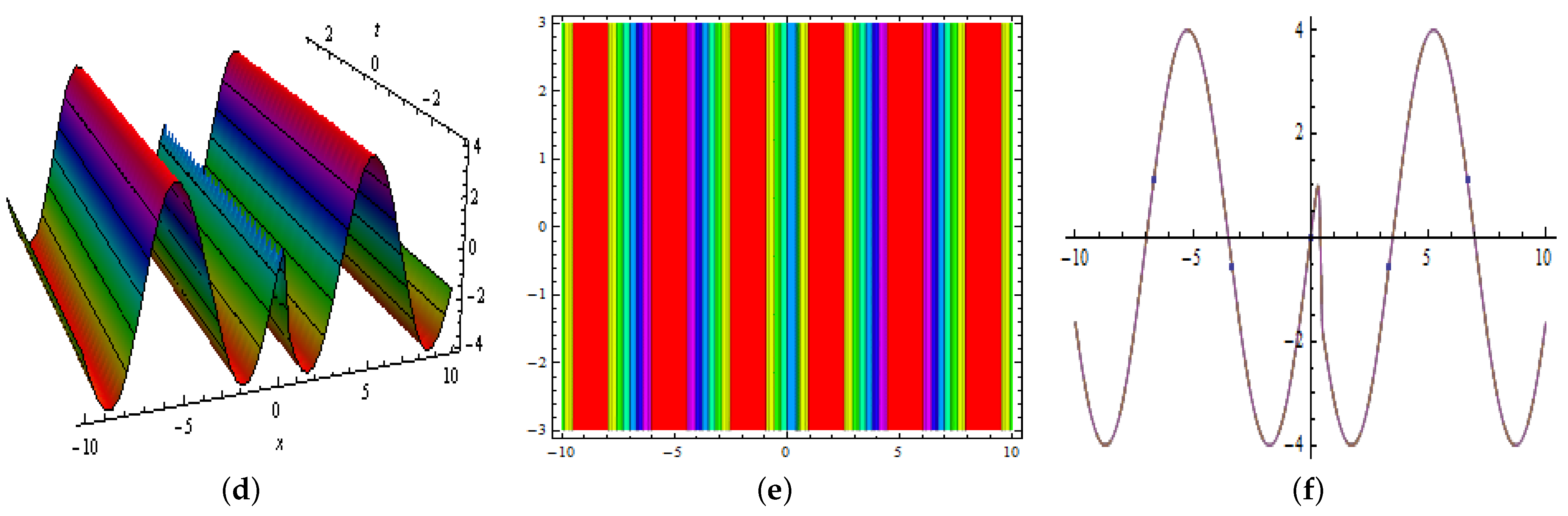
where all are real-valued parameters to be measured. Inserting into Equation (11) and collecting all powers of , , , , , , , , and , we obtain proper results, as follows (See Figure 3, Figure 4, Figure 5 and Figure 6):
Set I. For ,
and
Set II. For ,
Set III. For ,
and
3.2. Two-Kink Soliton
For two-kink interaction, the bilinear solution for is as follows (See Figure 7, Figure 8 and Figure 9):
where and all are real-valued parameters to be found. Inserting into Equation (11) and collecting all powers of and , , , , , , , , , , , , we obtain proper results, as follows:
Set I. For ,
Set II.
3.3. Periodic Waves
For periodic-wave interaction solutions, the bilinear form for is as follows (See Figure 10 and Figure 11):
where and all are real-valued parameters to be found. Inserting into Equation (11) and collecting all powers of and , , , , , , , , , , we obtain proper results as follows:
Set I. For ,
By using these parameters in Equation (38), and then by using Equations (8) and (10), we obtain
Set II. For ,
4. Multiwave Solutions
For multiwave solutions, in bilinear form can be assumed as [32]
where and all are real-valued parameters to be measured. Inserting into Equation (11) and collecting all coefficients of , , , , , , , and , we obtain proper results, as follows (See Figure 12 and Figure 13):
Case I.
By using these values in Equation (44) and then by using Equations (8) and (10), we obtain
Case II.
By using these values in Equation (44) and then by using Equations (8) and (10), we obtain
5. Homoclinic Breather Approach
To obtain breather solutions, in bilinear form can be assumed as [32]
where p, q, , , and all are real-valued parameters to be found. Inserting into Equation (11) and collecting all coefficients of and , we obtain an algebraic system of equations, then, after solving them, we obtain proper results, as follows (See Figure 14 and Figure 15):
Case I.
By using these parameters in Equation (51) and then by using Equations (8) and (10), we obtain
.
Case II.
6. The Periodic Cross-Kink Wave Solutions
For this, in bilinear form can be assumed as [33]
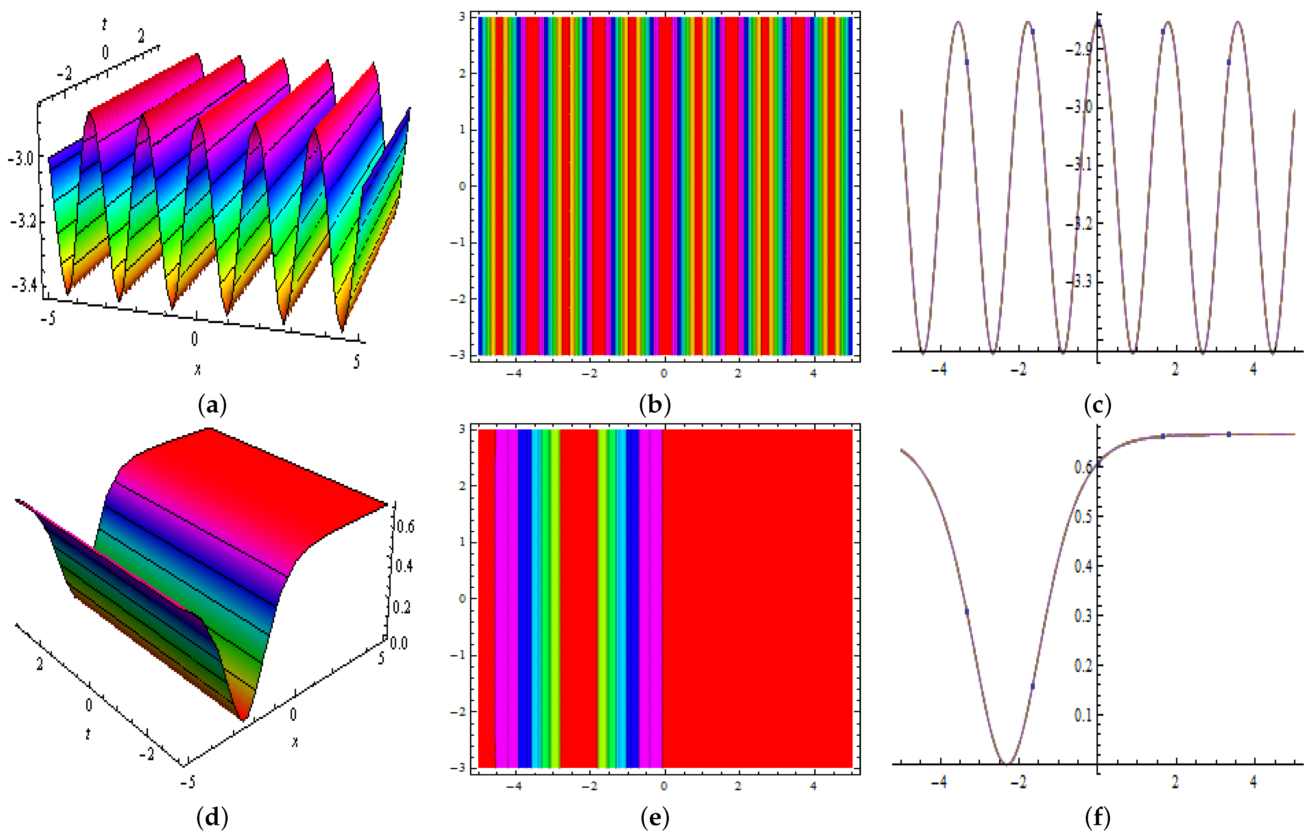
where and all are real-valued parameters to be measured. Inserting into Equation (11) and collecting all coefficients of , , and , after solving them, we attain the following parameters (See Figure 16 and Figure 17):
Case I. For
By using these values in Equation (57), and then by using Equations (8) and (10), we obtain
Case II.
7. Results and Discussion
The study of new imposed solutions for the ion sound and Langmuir waves (ISLWs) has huge importance among scientists. Much of the work has been carried out on ISLWs, for example, Mohammed et al. constructed new traveling wave solutions for ISLWs by using He’s semi-inverse and extended Jacobian elliptic function method [34]. Shakeel et al. studied new wave behaviors for ISLWs with the aid of modified exp-function approach [35]. Seadawy et al. used direct algebraic and auxiliary equation mapping to obtain the families of new exact traveling wave solutions for ISLWs [36]. Tripathy and Sahoo studied a variety of analytical solutions for ISLWs [37]. Seadawy et al. studied a variety of exact solutions with modified Kudraysov and hyperbolic-function scheme for ISLWs [38].
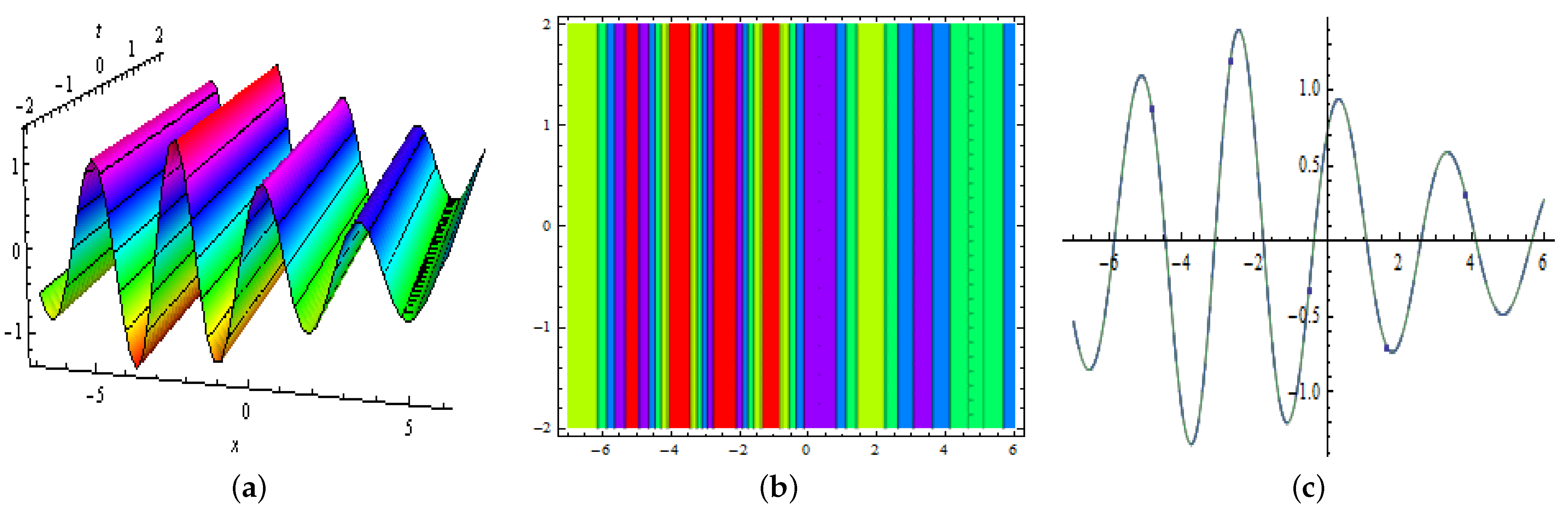
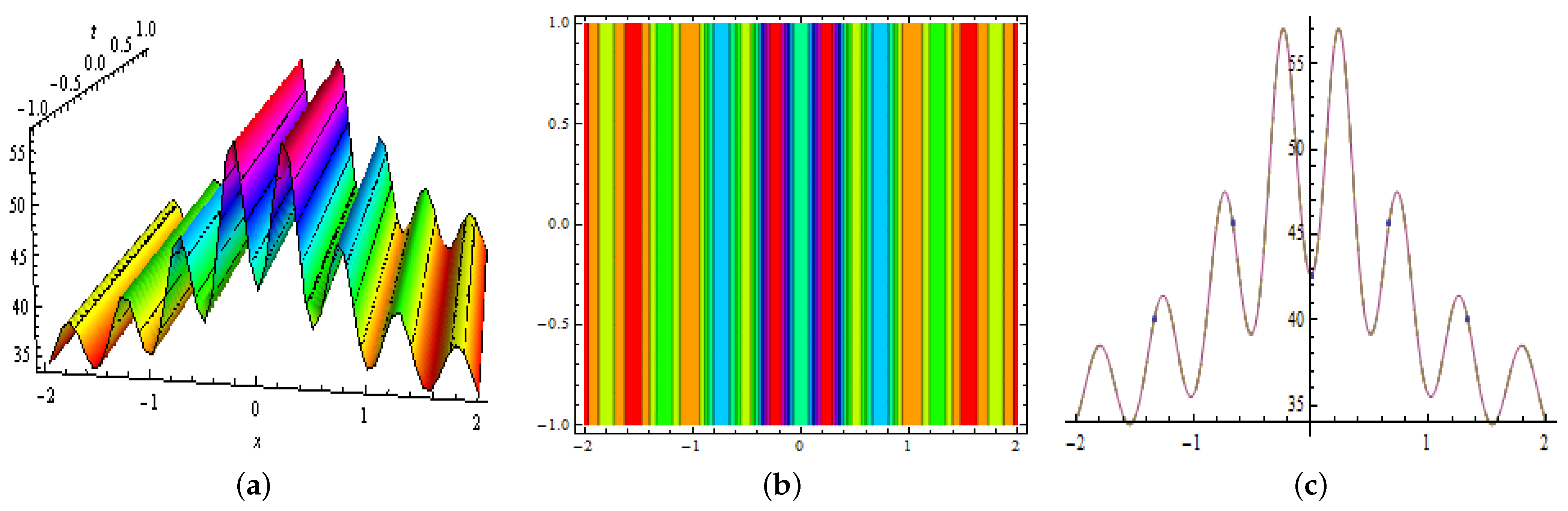
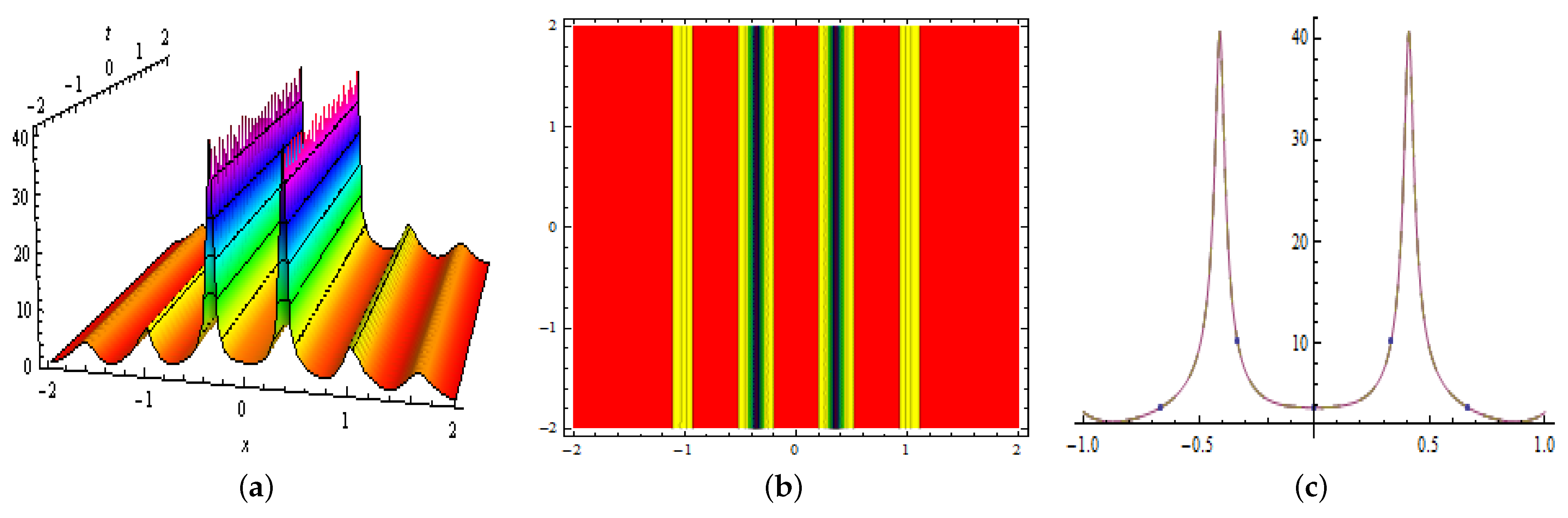
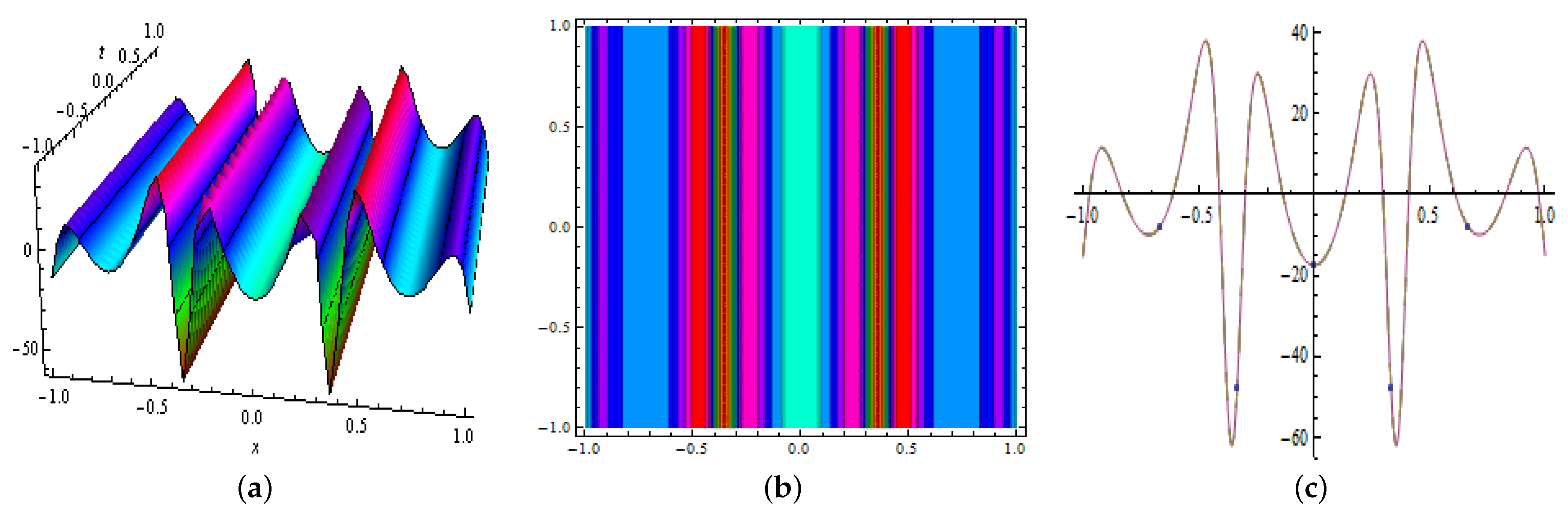
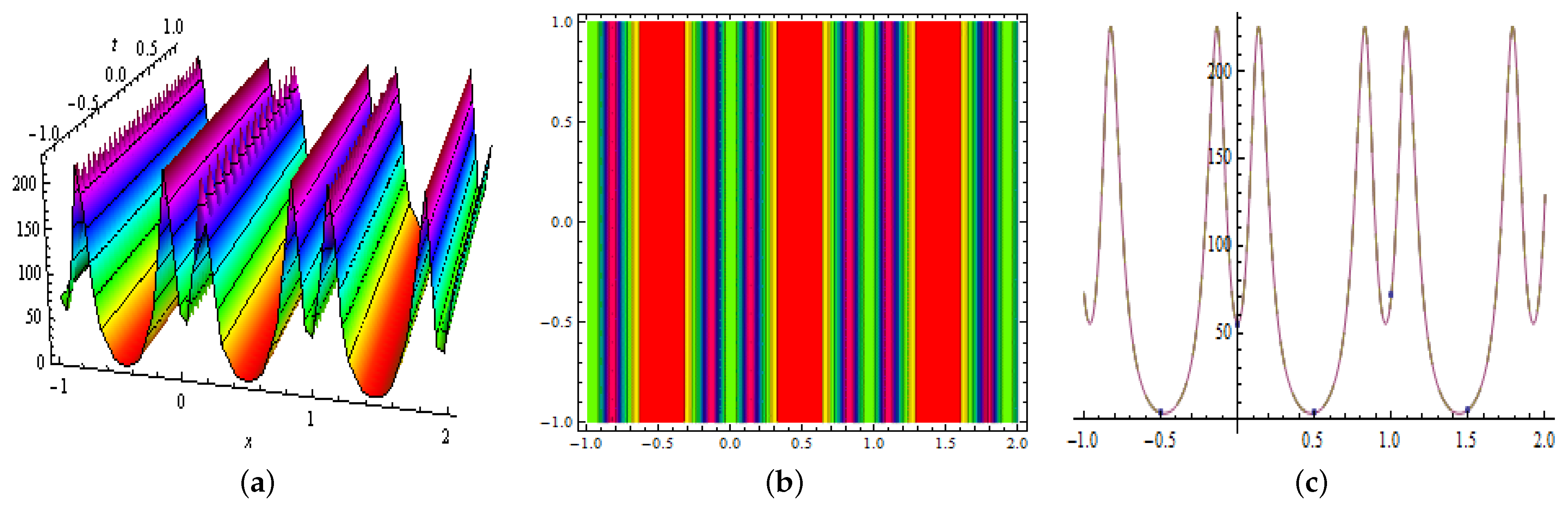
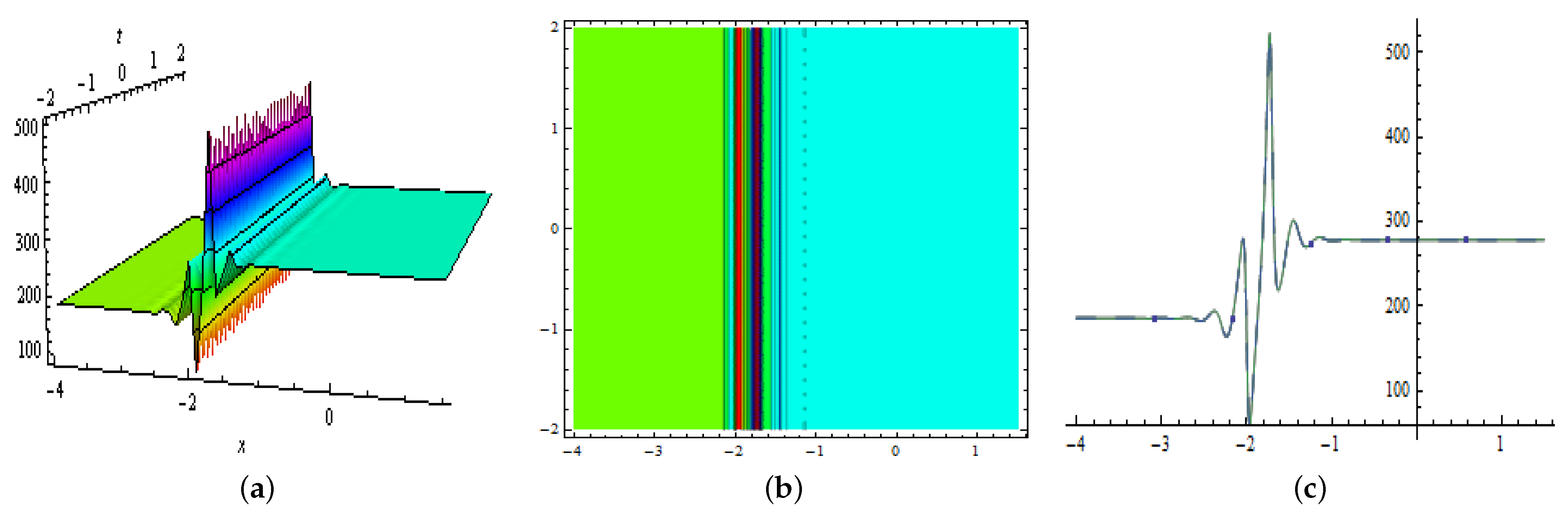
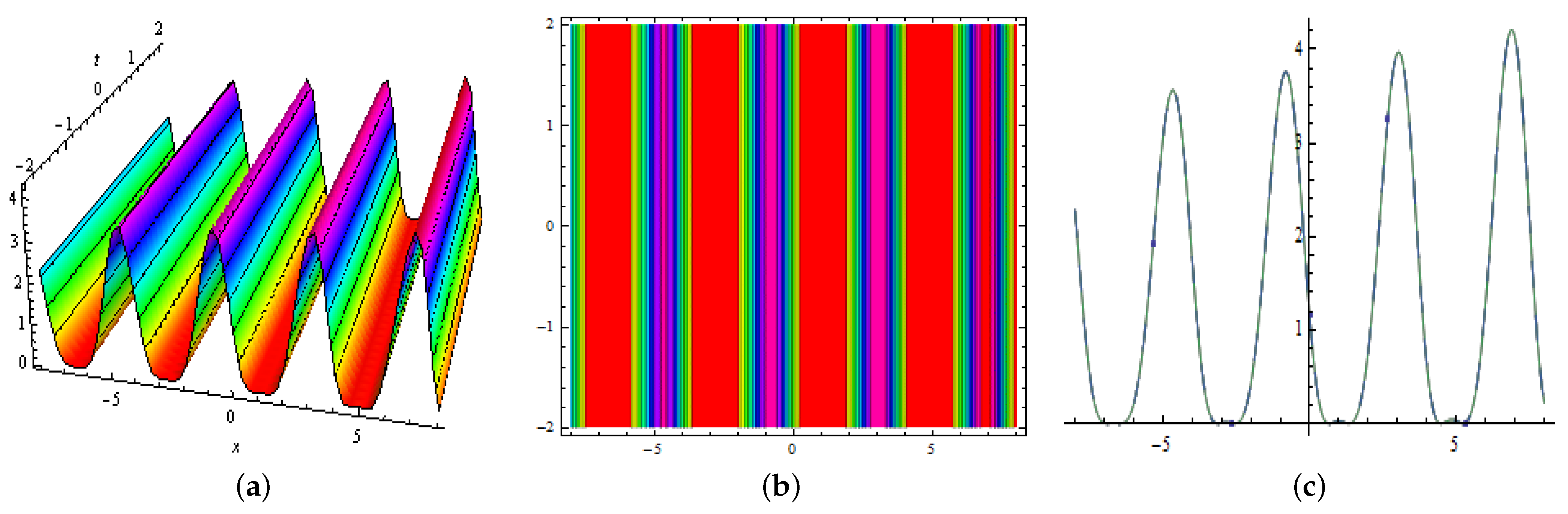
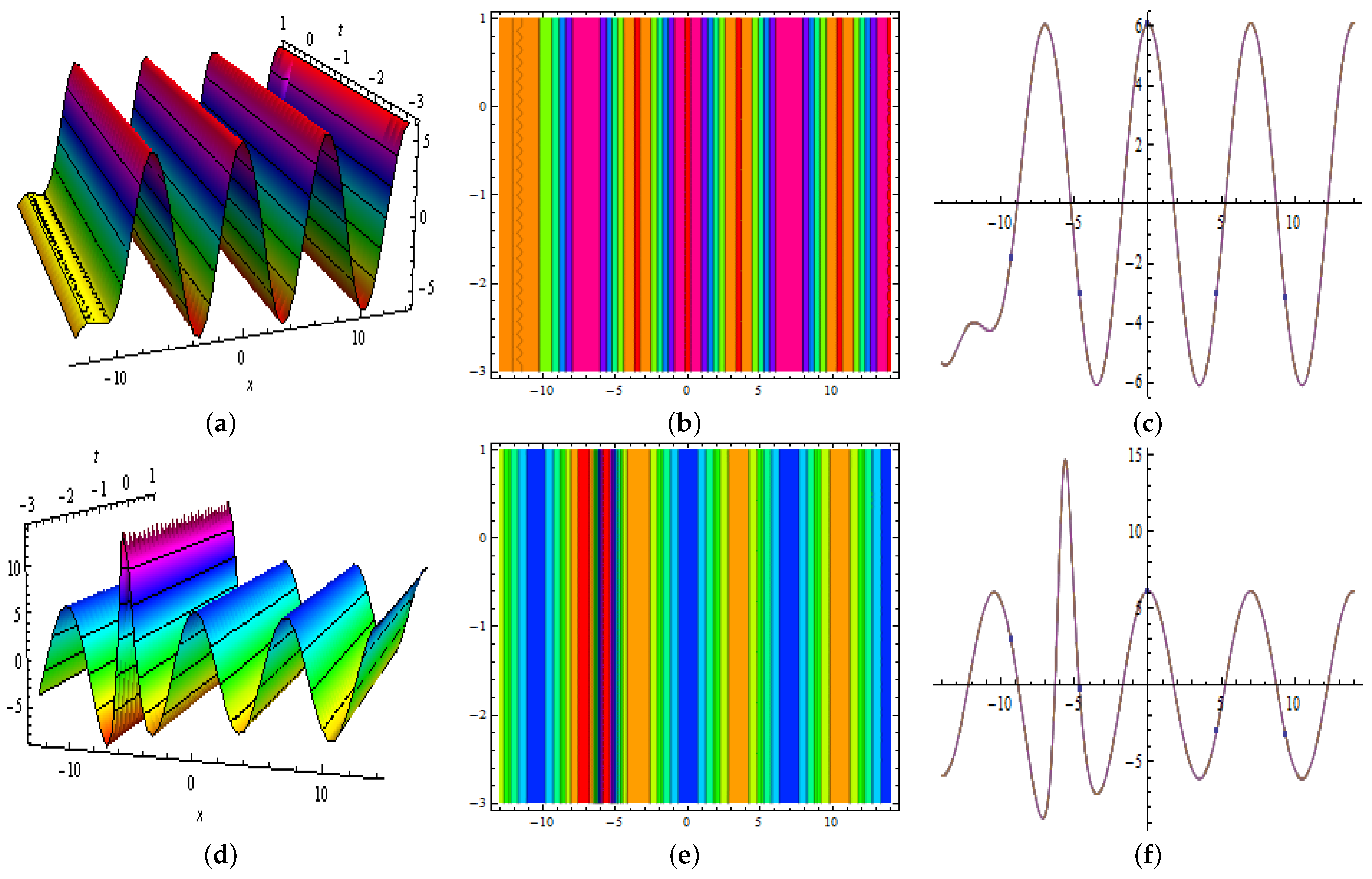
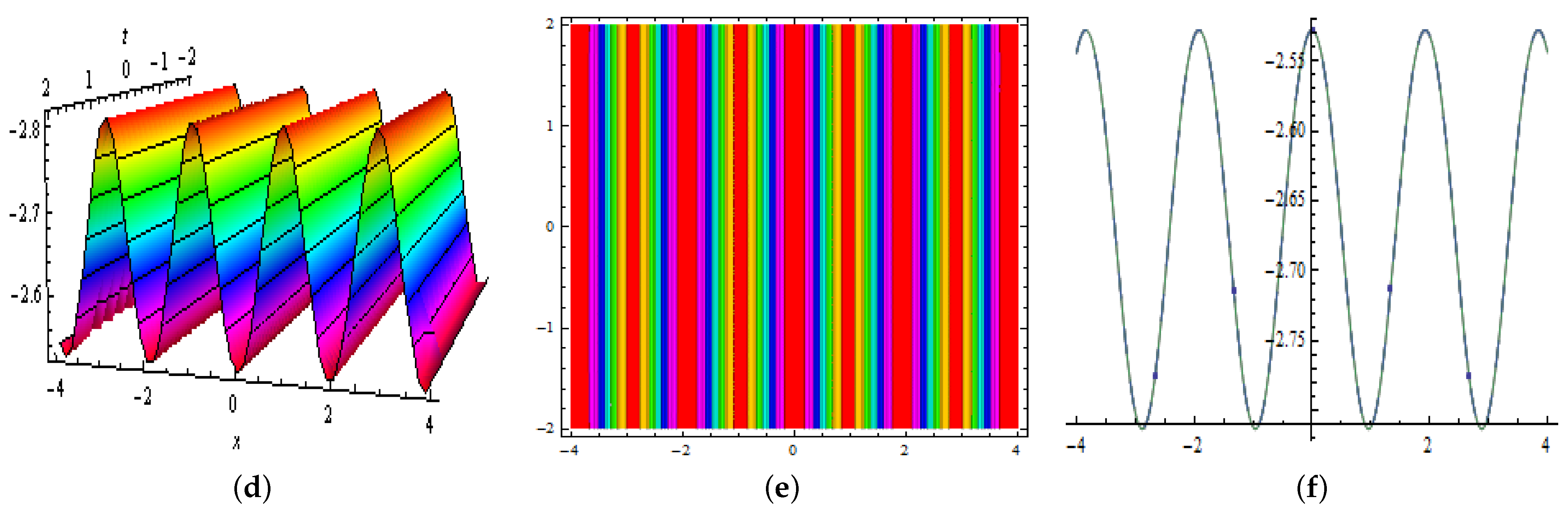
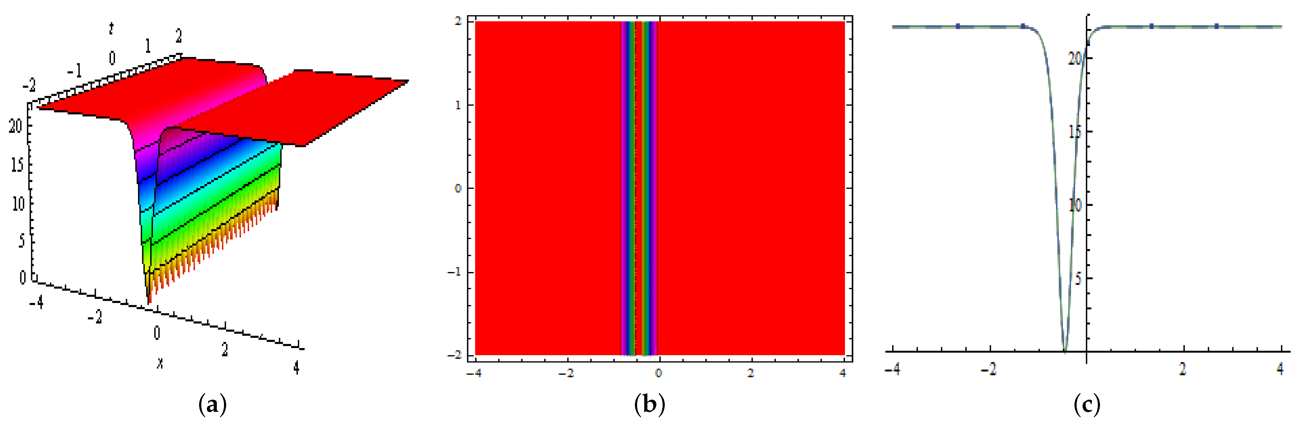
Here, we obtained a variety of analytical solutions with rational and trigonometric forms for ISLWs, in which some of them are represented graphically in 3D, contour, and 2D shapes. In Figure 1 and Figure 2, we present M-shaped solutions for and with contour and 2D plots, respectively. In Figure 3, Figure 4, Figure 5 and Figure 6, we see the interactional phenomena with M-shaped and one-kink for , , , and at different values of the parameters. In these figures, we see M-shaped waves with multiple bright and dark solutions. In Figure 4, waves strongly increased their amplitude according to time. In Figure 7, Figure 8 and Figure 9, we see the interactional phenomena with M-shaped and two-kink for , , and . In Figure 7, multiple bright, dark, and M-size solitons appear. In Figure 8 and Figure 9, large-sized dark and bright waves appear. Figure 10 and Figure 11 represent the evolution of M-shaped and periodic waves for and . Figure 12 and Figure 13 represent the evolution of multiwaves solution for and at different values. In Figure 14 and Figure 15, two solutions, and , of homoclinic breather are presented graphically, and we also see the changes in graphs by varying the value of a. In Figure 16 and Figure 17, we present periodic cross-kink solutions and graphically, and we also see the change in waves into bright and dark solutions by varying the value of a. As , in all these solutions, we can see that when , does not converge.
8. Conclusions
In this work, we successfully derived some new analytic solutions for FISLWS with Atangana–Baleanu derivative. These exact solutions are derived in the form of bilinear, trigonometric, and exponential functions. As a result, new traveling wave solutions are gained in the form of rational, periodic, multiwaves, multi-kink, solitary waves, bright and dark solitons that are shown graphically in 3D, 2D, and contour structures. These solutions play an important role in different areas of physics, engineering, and other branches of sciences.
Author Contributions
Methodology, S.T.R.R.; Resources, A.D.A.; Supervision, A.R.S.; Writing, S.A.O.B. All authors have read and agreed to the published version of the manuscript.
Funding
This research received no external funding.
Institutional Review Board Statement
Not applicable.
Informed Consent Statement
Not applicable.
Data Availability Statement
Not applicable.
Acknowledgments
This work was funded by the Deanship of Scientific Research at Jouf University under grant No (DSR-2021-03-03106).
Conflicts of Interest
The authors declare no conflict of interest.
References
- Dalir, M.; Bashour, M. Applications of Fractional Calculus. Appl. Math. Sci. 2010, 4, 1021–1032. [Google Scholar]
- Özkan, Y.S.; Seadawy, A.R.; Yaşar, E. Multi-wave, breather and interaction solutions to (3 + 1) dimensional Vakhnenko–Parkes equation arising at propagation of high-frequency waves in a relaxing medium. J. Taibah Univ. Sci. 2021, 15, 666–678. [Google Scholar] [CrossRef]
- Lu, D.; Seadawy, A.R.; Iqbal, M. Mathematical physics via construction of traveling and solitary wave solutions of three coupled system of nonlinear partial differential equations and their applications. Results Phys. 2018, 11, 1161–1171. [Google Scholar] [CrossRef]
- Seadawy, A.R.; Ali, A.; Albarakati, W.A. Analytical wave solutions of the (2 + 1)-dimensional first integro-differential Kadomtsev-Petviashivili hierarchy equation by using modified mathematical methods. Results Phys. 2019, 15, 102775. [Google Scholar] [CrossRef]
- Seadawy, A.R.; Cheemaa, N. Propagation of nonlinear complex waves for the coupled nonlinear Schrödinger Equations in two core optical fibers. Phys. A Stat. Mech. Its Appl. 2019, 529, 121330. [Google Scholar] [CrossRef]
- Kudryashov, N.A. The generalized Duffing oscillator. Commun. Nonlinear Sci. Numer. Simulat. 2021, 93, 105526. [Google Scholar] [CrossRef]
- Kudryashov, N.A. Model of propagation pulses in an optical fiber with a new law of refractive index. Optik 2021, 248, 168160. [Google Scholar] [CrossRef]
- Kudryashov, N.A. Solitary waves of the non-local Schrödinger equation with arbitrary refractive index. Optik 2021, 231, 166443. [Google Scholar] [CrossRef]
- Kudryashov, N.A. Almost general solution of the reduced higher-order nonlinear Schrödinger equation. Optik 2021, 230, 166347. [Google Scholar] [CrossRef]
- Kudryashov, N.A. Periodic and solitary waves in optical fiber Bragg gratings with dispersive reflectivity. Chin. J. Phys. 2020, 66, 401–405. [Google Scholar] [CrossRef]
- Rizvi, S.T.R.; Seadawy, A.R.; Younis, M.; Ahmad, N.; Zaman, S. Optical dromions for perturbed fractional nonlinear Schrödinger equation with conformable derivatives. Opt. Quantum Electron. 2021, 53, 477. [Google Scholar] [CrossRef]
- Younas, U.; Younis, M.; Seadawy, A.R.; Rizvi, S.T.R.; Althobaiti, S.; Sayed, S. Diverse exact solutions for modified nonlinear Schrödinger equation with conformable fractional derivative. Results Phys. 2021, 20, 103766. [Google Scholar] [CrossRef]
- Mohammadi, H.; Kumar, S.; Rezapour, S.; Etemad, S. A theoretical study of the Caputo–Fabrizio fractional modeling for hearing loss due to Mumps virus with optimal control. Chaos Solitons Fractals 2021, 144, 110668. [Google Scholar] [CrossRef]
- Nisar, K.S.; Jothimani, K.; Kaliraj, K.; Ravichandran, C. An analysis of controllability results for nonlinear Hilfer neutral fractional derivatives with non-dense domain. Chaos Solitons Fractals 2021, 146, 110915. [Google Scholar] [CrossRef]
- Kaliraj, K.; Thilakraj, E.; Ravichandran, C.; Nisar, K.S. Controllability analysis for impulsive integro-differential equation via Atangana–Baleanu fractional derivative. Math. Methods Appl. Sci. 2020. [Google Scholar] [CrossRef]
- Panda, S.K.; Ravichandran, C.; Hazarika, B. Ravichandran, Bipan Hazarika, Results on system of Atangana–Baleanu fractional order Willis aneurysm and nonlinear singularly perturbed boundary value problems. Chaos Solitons Fractals 2021, 142, 110390. [Google Scholar] [CrossRef]
- Younas, U.; Seadawy, A.R.; Younis, M.; Rizvi, S. Construction of analytical wave solutions to the conformable fractional dynamical system of ion sound and Langmuir waves. Waves Random Complex Media 2020, 32, 1–19. [Google Scholar] [CrossRef]
- Akram, U.; Seadawy, A.R.; Rizvi, S.T.R.; Younis, M.; Althobaiti, S.; Sayed, S. Traveling waves solutions for the fractional Wazwaz Benjamin Bona Mahony model in arising shallow water waves. Results Phys. 2021, 20, 103725. [Google Scholar] [CrossRef]
- Dokuyucua, M.A. Caputo and Atangana-Baleanu-Caputo Fractional Derivative Applied to Garden Equation. Turk. J. Sci. 2020, 5, 1–7. [Google Scholar]
- Seadawy, A.R. Modulation instability analysis for the generalized derivative higher order nonlinear Schrödinger equation and its the bright and dark soliton solutions. J. Electromagn. Waves Appl. 2017, 31, 1353–1362. [Google Scholar] [CrossRef]
- Zhang, S.; Zong, Q.A.; Liu, D.; Gao, Q. A generalized exp-function method for fractional Riccati differential equations. Commun. Fract. Calc. 2010, 1, 48–51. [Google Scholar]
- Seadawy, A.R.; Tariq, K.U. On some novel solitons to the generalized (1 + 1)-dimensional unstable spacetime fractional nonlinear Schrödinger model emerging in the optical fibers. Opt. Quantum Electron. 2021, 53, 1–16. [Google Scholar] [CrossRef]
- Chen, C.; Jiang, Y.; Wang, Z.; Wu, J. Dynamical behavior and exact solutions for time-fractional nonlinear Schrödinger equation with parabolic law nonlinearity. Optik 2020, 222, 165331. [Google Scholar] [CrossRef]
- Khan, S.A.; Shah, K.; Kumam, P.; Seadawy, A.; Zaman, G.; Shah, Z. Study of mathematical model of Hepatitis B under Caputo-Fabrizo derivative. AIMS Math. 2021, 6, 195–209. [Google Scholar] [CrossRef]
- Seadawy, A.R.; Bilal, M.; Younis, M.; Rizvi, S.; Althobaiti, S.; Makhlouf, M. Analytical mathematical approaches for the double-chain model of DNA by a novel computational technique. Chaos Solitons Fractals 2021, 144, 110669. [Google Scholar] [CrossRef]
- Farah, N.; Seadawy, A.R.; Ahmad, S.; Rizvi, S.T.R.; Younis, M. Interaction properties of soliton molecules and Painleve analysis for nano bioelectronics transmission model. Opt. Quantum Electron. 2020, 52, 1–15. [Google Scholar] [CrossRef]
- Helal, M.A.; Seadawy, A.R. Variational method for the derivative nonlinear Schrödinger equation with computational applications. Phys. Scr. 2009, 80, 350–360. [Google Scholar] [CrossRef]
- Gaber, A.A.; Aljohani, A.F.; Ebaid, A.; Machado, J.T. The generalized Kudryashov method for nonlinear space-time fractional partial differential equations of Burgers type. Nonlinear Dyn. 2019, 95, 361–368. [Google Scholar] [CrossRef]
- Ghaffar, A.; Ali, A.; Ahmed, S.; Akram, S.; Junjua, M.-U.-D.; Baleanu, D.; Nisar, K.S. A novel analytical technique to obtain the solitary solutions for nonlinear evolution equation of fractional order. Adv. Differ. Equ. 2020, 2020, 308. [Google Scholar] [CrossRef]
- Rizvi, S.T.R.; Ali, K.; Ahmad, M. Optical solitons for Biswas–Milovic equation by new extended auxiliary equation method. Optik 2020, 204, 164181. [Google Scholar] [CrossRef]
- Ahmed, I.; Seadawy, A.R.; Lu, D. M-shaped rational solitons and their interaction with kink waves in the Fokas–Lenells equation. Phys. Scr. 2019, 94, 055205. [Google Scholar] [CrossRef]
- Ahmed, I.; Seadawy, A.R.; Lu, D. Kinky breathers, W-shaped and multi-peak solitons interaction in (2 + 1)-dimensional nonlinear Schrödinger equation with Kerr law of nonlinearity. Eur. Phys. J. Plus 2019, 134, 120. [Google Scholar] [CrossRef]
- Ma, H.; Zhang, C.; Deng, A. New Periodic Wave, Cross-Kink Wave, Breather, and the Interaction Phenomenon for the (2+1)-Dimensional Sharmo–Tasso–Olver Equation. Complexity 2020, 2020, 4270906. [Google Scholar] [CrossRef]
- Mohammed, W.W.; Abdelrahman, M.A.E.; Inc, M.; Hamza, A.E.; Akinlar, M.A. Soliton solutions for system of ion sound and Langmuir waves. Opt. Quantum Electron. 2020, 52, 1–10. [Google Scholar] [CrossRef]
- Shakeel, M.; Iqbal, M.A.; Din, Q.; Hassan, Q.M.; Ayub, K. New exact solutions for coupled nonlinear system of ion sound and Langmuir waves. Indian J. Phys. 2019, 94, 885–894. [Google Scholar] [CrossRef]
- Seadawy, A.R.; Lu, D.; Iqbal, M. Application of mathematical methods on the system of dynamical equations for the ion sound and Langmuir waves. Pramana 2019, 93, 1–12. [Google Scholar] [CrossRef]
- Tripathy, A.; Sahoo, S. Exact solutions for the ion sound Langmuir wave model by using two novel analytical methods. Results Phys. 2020, 19, 103494. [Google Scholar] [CrossRef]
- Seadawy, A.R.; Kumar, D.; Hosseini, K.; Samadani, F. The system of equations for the ion sound and Langmuir waves and its new exact solutions. Results Phys. 2018, 9, 1631–1634. [Google Scholar] [CrossRef]
Figure 1.
Plots of in Equation (17) for , respectively as three-dimensions in (a); contour in (b) and two-dimensions in (c).
Figure 1.
Plots of in Equation (17) for , respectively as three-dimensions in (a); contour in (b) and two-dimensions in (c).
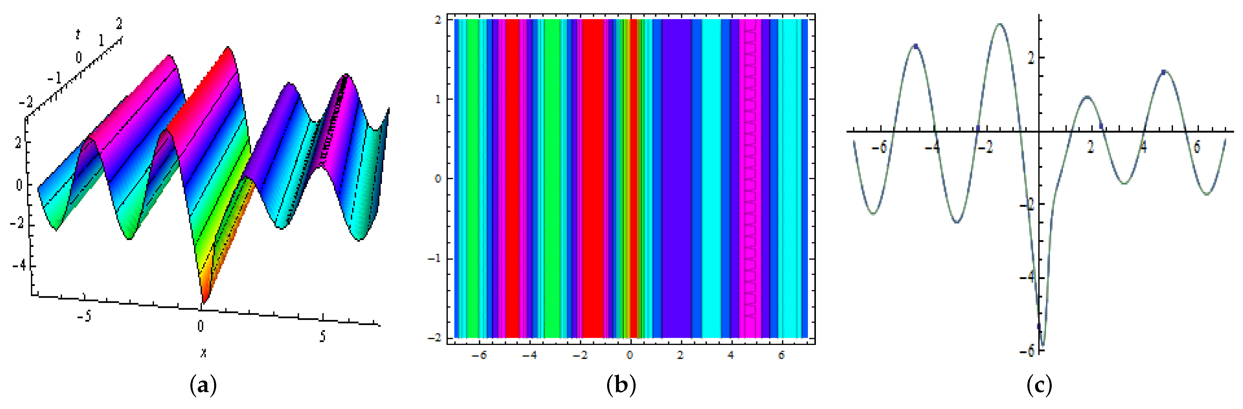
Figure 2.
Represented three-dimensions in (a); contour in (b) and two-dimensions in (c), Plots of in Equation (20) for , respectively.
Figure 2.
Represented three-dimensions in (a); contour in (b) and two-dimensions in (c), Plots of in Equation (20) for , respectively.

Figure 3.
Showed three-dimensions in (a); contour in (b) and two-dimensions in (c), Plots of in Equation (24) for , respectively.
Figure 3.
Showed three-dimensions in (a); contour in (b) and two-dimensions in (c), Plots of in Equation (24) for , respectively.
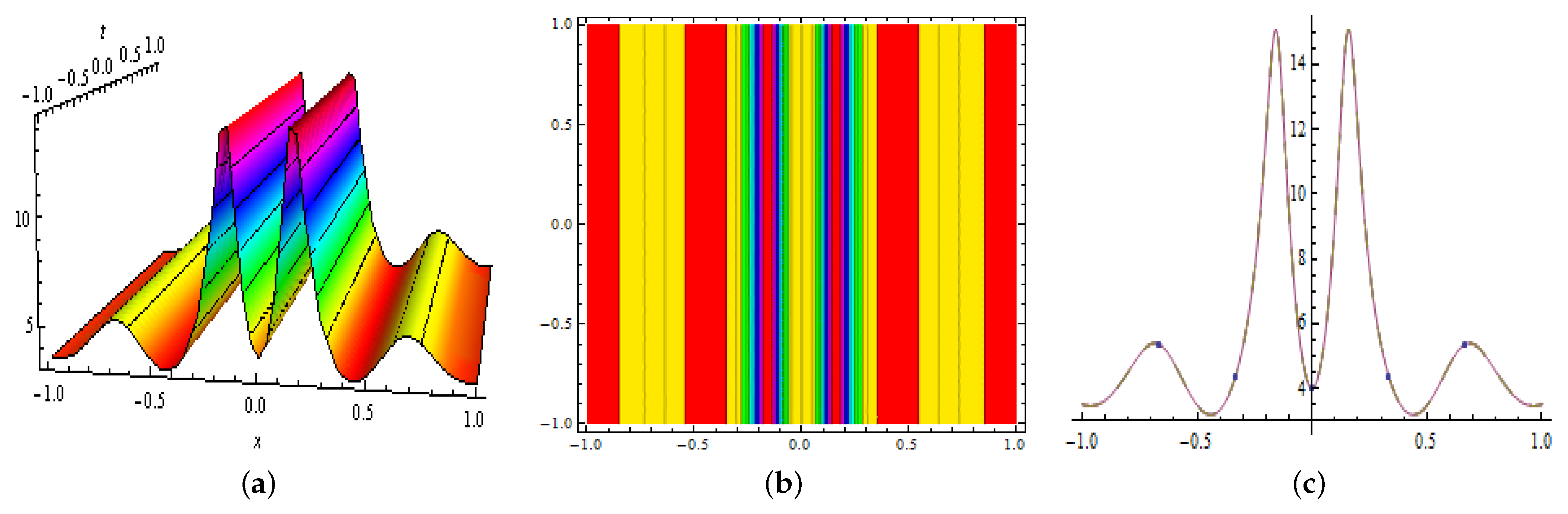
Figure 4.
Illustrated three-dimensions in (a); contour in (b) and two-dimensions in (c), Plots of in Equation (24) for , respectively.
Figure 4.
Illustrated three-dimensions in (a); contour in (b) and two-dimensions in (c), Plots of in Equation (24) for , respectively.

Figure 5.
Clarify three-dimensions in (a); contour in (b) and two-dimensions in (c), Plots of in Equation (30) for , respectively.
Figure 5.
Clarify three-dimensions in (a); contour in (b) and two-dimensions in (c), Plots of in Equation (30) for , respectively.

Figure 6.
Explain three-dimensions in (a); contour in (b) and two-dimensions in (c), Plots of in Equation (30) for , respectively.
Figure 6.
Explain three-dimensions in (a); contour in (b) and two-dimensions in (c), Plots of in Equation (30) for , respectively.

Figure 7.
Represented three-dimensions in (a); contour in (b) and two-dimensions in (c), Plots of in Equation (34) for , respectively.
Figure 7.
Represented three-dimensions in (a); contour in (b) and two-dimensions in (c), Plots of in Equation (34) for , respectively.

Figure 8.
Showed three-dimensions in (a); contour in (b) and two-dimensions in (c), Plots of in Equation (37) for , respectively.
Figure 8.
Showed three-dimensions in (a); contour in (b) and two-dimensions in (c), Plots of in Equation (37) for , respectively.
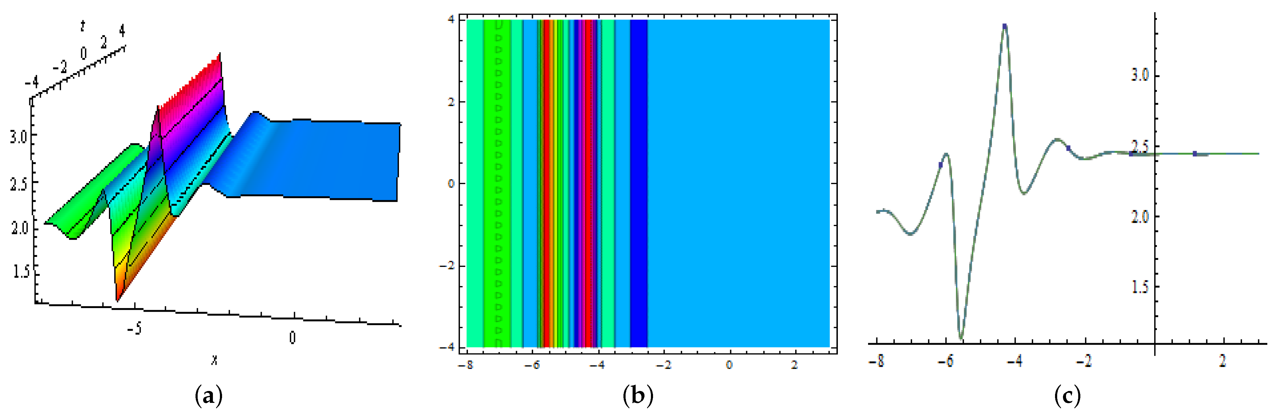
Figure 9.
Illustrated three-dimensions in (a); contour in (b) and two-dimensions in (c), Plots of in Equation (37) for , respectively.
Figure 9.
Illustrated three-dimensions in (a); contour in (b) and two-dimensions in (c), Plots of in Equation (37) for , respectively.

Figure 10.
Showed three-dimensions in (a); contour in (b) and two-dimensions in (c), Plots of in Equation (43) at , respectively.
Figure 10.
Showed three-dimensions in (a); contour in (b) and two-dimensions in (c), Plots of in Equation (43) at , respectively.
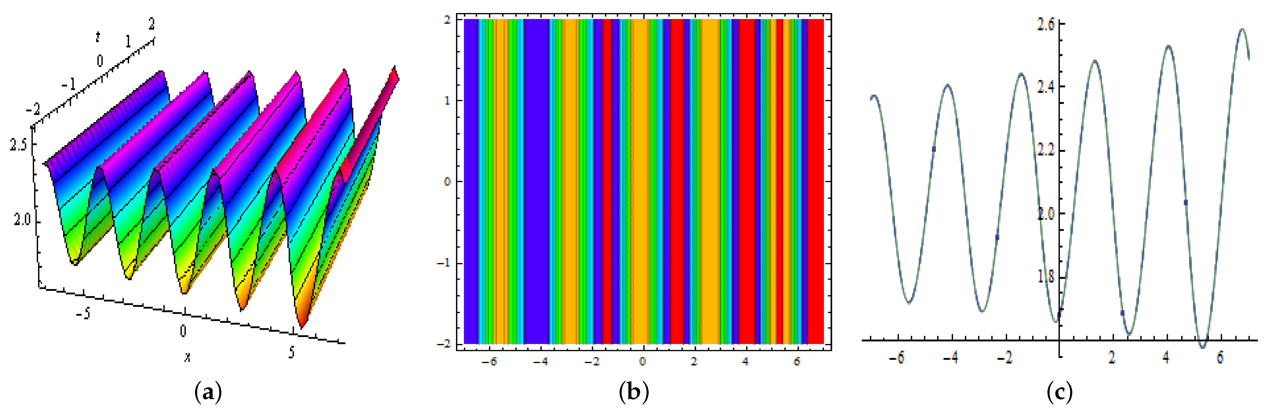
Figure 11.
Represented three-dimensions in (a); contour in (b) and two-dimensions in (c), Plots of in Equation (43) at , respectively.
Figure 11.
Represented three-dimensions in (a); contour in (b) and two-dimensions in (c), Plots of in Equation (43) at , respectively.

Figure 12.
Showed three-dimensions in (a); contour in (b) and two-dimensions in (c), Graphical representation of in Equation (50), for , respectively.
Figure 12.
Showed three-dimensions in (a); contour in (b) and two-dimensions in (c), Graphical representation of in Equation (50), for , respectively.

Figure 13.
Represented three-dimensions in (a); contour in (b) and two-dimensions in (c), Graphical representation of in Equation (50), for , respectively.
Figure 13.
Represented three-dimensions in (a); contour in (b) and two-dimensions in (c), Graphical representation of in Equation (50), for , respectively.

Figure 14.
Explain three-dimensions in (a); contour in (b) and two-dimensions in (c), Graphical representation of in Equation (54), at , respectively.
Figure 14.
Explain three-dimensions in (a); contour in (b) and two-dimensions in (c), Graphical representation of in Equation (54), at , respectively.


Figure 15.
Clarify three-dimensions in (a); contour in (b) and two-dimensions in (c), Graphical representation of in Equation (56), at , successively.
Figure 15.
Clarify three-dimensions in (a); contour in (b) and two-dimensions in (c), Graphical representation of in Equation (56), at , successively.

Figure 16.
Showed three-dimensions in (a); contour in (b) and two-dimensions in (c), Graphical representation of in Equation (62), for , respectively.
Figure 16.
Showed three-dimensions in (a); contour in (b) and two-dimensions in (c), Graphical representation of in Equation (62), for , respectively.
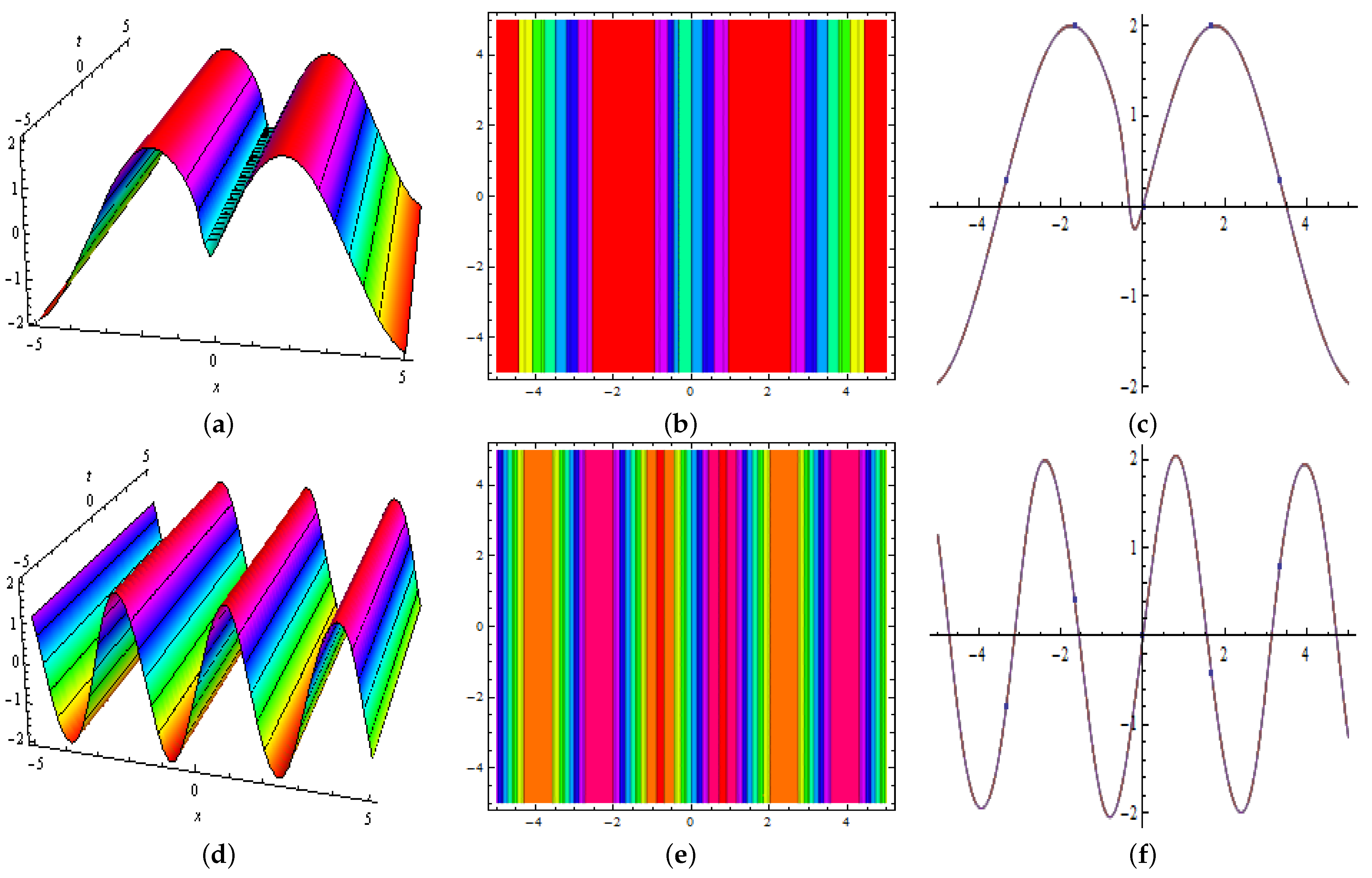
Figure 17.
Represented three-dimensions in (a); contour in (b) and two-dimensions in (c), Graphical representation of in Equation (62), for , respectively.
Figure 17.
Represented three-dimensions in (a); contour in (b) and two-dimensions in (c), Graphical representation of in Equation (62), for , respectively.

Publisher’s Note: MDPI stays neutral with regard to jurisdictional claims in published maps and institutional affiliations. |
© 2022 by the authors. Licensee MDPI, Basel, Switzerland. This article is an open access article distributed under the terms and conditions of the Creative Commons Attribution (CC BY) license (https://creativecommons.org/licenses/by/4.0/).
Share and Cite
MDPI and ACS Style
Alruwaili, A.D.; Seadawy, A.R.; Rizvi, S.T.R.; Beinane, S.A.O. Diverse Multiple Lump Analytical Solutions for Ion Sound and Langmuir Waves. Mathematics 2022, 10, 200. https://doi.org/10.3390/math10020200
AMA Style
Alruwaili AD, Seadawy AR, Rizvi STR, Beinane SAO. Diverse Multiple Lump Analytical Solutions for Ion Sound and Langmuir Waves. Mathematics. 2022; 10(2):200. https://doi.org/10.3390/math10020200
Chicago/Turabian StyleAlruwaili, Abdulmohsen D., Aly R. Seadawy, Syed T. R. Rizvi, and Sid Ahmed O. Beinane. 2022. "Diverse Multiple Lump Analytical Solutions for Ion Sound and Langmuir Waves" Mathematics 10, no. 2: 200. https://doi.org/10.3390/math10020200
Note that from the first issue of 2016, this journal uses article numbers instead of page numbers. See further details here.