
Introducing Two Parsimonious Standard Power Mixture Models for Bimodal Proportional Data with Application to Loss Given Default


1
Centre for Business Mathematics and Informatics, North-West University, Potchefstroom 2531, South Africa
2
School of Mathematical and Statistical Sciences, North-West University, Potchefstroom 2531, South Africa
*
Author to whom correspondence should be addressed.
†
These authors contributed equally to this work.
Mathematics 2022, 10(23), 4520; https://doi.org/10.3390/math10234520
Submission received: 26 September 2022
/
Revised: 10 November 2022
/
Accepted: 17 November 2022
/
Published: 30 November 2022
(This article belongs to the Section Probability and Statistics)
Abstract
:The need to model proportional data is common in a range of disciplines however, due to its bimodal nature, U- or J-shaped data present a particular challenge. In this study, two parsimonious mixture models are proposed to accurately characterise this proportional U- and J-shaped data. The proposed models are applied to loss given default data, an application area where specific importance is attached to the accuracy with which the mean is estimated, due to its linear relationship with a bank’s regulatory capital. In addition to using standard information criteria, the degree to which bias reduction in the estimation of the distributional mean can be achieved is used as a measure of model performance. The proposed models outperform the benchmark model with reference to the information criteria and yield a reduction in the distance between the empirical and distributional means. Given the special characteristics of the dataset, where a high proportion of observations are close to zero, a methodology for choosing a rounding threshold in an objective manner is developed as part of the data preparation stage. It is shown how the application of this rounding threshold can reduce bias in moment estimation regardless of the model choice.
Keywords:
proportional bimodal data; parsimonious model; mixture model; rounding threshold; standard power distributionMSC:
62P051. Introduction
The need to model proportional data is common in a wide range of disciplines, including the fields of economics, biometrics, as well as social and political sciences [1]. With proportional (or fractional) data, the variable of interest takes on values in the range and bi- or multi-modality is commonly observed.
Given its characteristics and its flexibility to represent a variety of shapes, the beta distribution has been widely used for the modelling of continuous, proportional data, bounded between 0 and 1. For example, in 1974, Falls [2] reinforced this notion in a study related to global cloud cover, by stating that “the beta distribution possesses the versatile statistical characteristics necessary to assume the wide variety of shapes exhibited by global cloud cover”. In a biological study, Kousathanas and Keightley [3] also proposed the use of beta distribution to model the bimodal nature of protein-coding loci, where amino-acid changing mutations are either neutral or strongly deleterious. In [4], the beta distribution is used to describe the distribution of consumer probabilities to purchase a brand in a consumer market. In credit risk, beta distribution has long been a popular choice for the modelling of loss given default (LGD) data, as can be seen, e.g., in [5,6,7]. LGD refers to the fraction of a loan that is not recovered in the case of default and it is usual for LGD to fall in the range , where 0 represents a full recovery and 1 represents a total loss of the outstanding amount. Finite mixtures of discretised beta distributions have also been proposed in the literature to deal with data that converge towards one of two opposing sides (this is referred to as polarisation in the literature, as can be seen, e.g., in [8]. Furthermore, Simone and Tutz [9], for example, proposed a mixture of binomial and discretised beta distributions to model uncertainty and response styles in ordinal data.
The ability of the beta distribution to provide a good fit to bimodal data mainly emerges in applications where frequency distributions exhibit either a U-shape or a J-shape, as can be seen, e.g., in [3,4,10,11]. However, beta densities that exhibit U-shapes have asymptotes at 0 and 1, potentially leading to an overestimation of the masses near the endpoints. Related to this property, the masses at the endpoints have an undue impact on the estimated parameters of the fitted beta distribution using maximum likelihood estimation (MLE), leading to adverse effects in the estimation of the moments of the fitted distribution, and most notably the mean and skewness where significant bias could be present. An unbiased mean is of particular importance for our application area, namely LGD modelling, because of the linear relationship between the LGD parameter and a bank’s regulatory capital, as prescribed by the Basel Committee on Banking Supervision ([12]). To overcome this problem, alternative distributions that provide a better fit, specifically at the end points, can be explored. Cognisant of the importance of an unbiased mean, we entertain a slight but necessary diversion in our study to address a practical problem commonly encountered in the modelling of LGD data. This relates to the undue impact that a high concentration of values very close to zero has on the estimation of the mean. As a secondary objective to our study, we therefore investigate a data preparation approach to choose a threshold below which values may be rounded to zero. We first demonstrate that rounding greatly reduces bias in mean estimation, and thereafter demonstrate an approach to choose such a rounding threshold in an objective manner.
Having addressed this practical data preparation challenge, we propose two distributions to more accurately model the U- and J-shaped LGD data while favouring parsimony and simplicity. In addition to an improved fit, our proposed models further reduce the bias in the estimation of the mean.
The remainder of the article is organised as follows. In Section 2, we introduce our benchmark model, the zero-one inflated beta distribution, and describe the characteristics of our data, before evaluating the performance of the fitted benchmark model. We also discuss an approach to handle trivial observations close to the boundaries and propose an objective approach to select an appropriate rounding threshold. Alternative models are then proposed in Section 3, the performance of which is evaluated using traditional information criteria both for our observed sample as well as in a bootstrap simulation study for small samples. We also propose and motivate an alternative approach to measure model performance, which has specific relevance for our application to LGD data. Section 4 concludes the paper and outlines some ideas for future work.
2. Data and Benchmark Model
In this section, we introduce our benchmark model, which we will refer to as the zero-one inflated beta distribution, before briefly describing the dataset used in this study. We then demonstrate the importance of rounding very small observations to zero during the data preparation phase in order to reduce bias and propose an objective approach for choosing the rounding threshold. Section concludes with an evaluation of the fit of our benchmark model.
2.1. Zero-One Inflated Beta Distribution
For LGD data, a high concentration of observations is typically observed at the boundaries, i.e., at total recovery and total loss. Zero-one inflated models are ideally suited to handle this phenomenon, as proposed by Ospina and Ferrari [13], who made use of the beta distribution to capture the distribution in the open interval . The authors motivate the use of the beta distribution based on its ability to model a variety of distributional shapes. Calabrese and Zenga [14] used Ospina and Ferrari [13]’s zero-one inflated beta (ZOIB) distribution to model the recovery rate of loans as the mixture of a Bernoulli random variable and a beta random variable.
In general, if a random variable X with density f is distributed as a zero-one inflated distribution, then
where is a mass function, is a density function, and is the mixture parameter. The mass function is that of a Bernoulli random variable, given by
where p represents the proportion of discrete observations (i.e., 0 or 1) with a value of 1.
In what follows, we will investigate a number of different choices for the density , which is used to model observations in the interval . The benchmark distribution is obtained when is the beta distribution with density function
with shape parameters and where is the gamma function, defined by
2.2. Data
The LGD data (i.e., the proportion of an individual loan account not recovered after default) used in this study to illustrate the methods proposed were obtained from an unsecured retail portfolio of a large South African bank. The period from January 2008 to April 2009 (16 months) was selected, resulting in more than 140,000 defaulted loan accounts. The choice of dates was motivated by default rates peaking over the reference period, which means that the LGD data reflect downturn conditions. The Basel Capital Accord mandates the use of LGD parameters that “reflect economic downturn conditions” for the determination of regulatory capital, as can be seen in [15]. Figure 1 below shows the distribution of LGD over the observation period, with the light blue bars representing a boxplot of data for each month. Due to confidentiality requirements, no actual values are shown. All figures and numerical results were developed in MATLAB version R2020a.
The solid dark blue line and lighter blue dashed line in Figure 1 were fitted through the mean and median LGD for each month, respectively, and indicate that LGD remained fairly stable over the reference period. The considerable distance between the plotted median and mean values is indicative of a left-skewed distribution, explained by a high concentration of observations at and close to 1. This is also evident from the proximity of the 75th percentile to 1.
The high concentration of values at 1, suggested by Figure 1, is confirmed in Figure 2, where the proportions of LGD observations at 1, 0, and on the interval (0, 1) are shown.
For illustrative purposes, the observations on (0, 1) are separated into observations in the (0, 0.01) and [0.01, 1) intervals, as indicated by the diamond markers within the sky blue bar. As can be observed, the proportion of observations between 0 and 0.01 exceeds that at 0 in each month considered.
In addition to having high concentrations of observations at the boundaries, it is common for proportional data to also exhibit high concentrations of values close to the boundary values. The substantial proportion of observations close to 0 and 1 in LGD data can in most cases be attributed to the effects of rounding during the collection and accounting processes. Specifically, accounting practices often result in trivial loss amounts being recorded for fully settled accounts.
In practice, values close to 0 and 1 are normally rounded during the data preparation stage, and the thresholds below or above which values are rounded are mostly chosen in an arbitrary manner. In the next section, we demonstrate the importance of rounding and show how a rounding threshold can be chosen in a more objective manner.
2.3. Selection of a Rounding Threshold
The benchmark ZOIB model defined in (1) to (3) was fitted to the LGD data using maximum likelihood estimation by applying MATLAB’s “betafit" function. The parameter estimates , , , and of the parameters w, p, , and are shown in Table 1 (recall that and is the shape parameters of the beta distribution, p is the probability of success in the Bernoulli distribution, and w is the mixing parameter). The stability of parameter estimates from month to month confirms our initial observation of homogeneity between the months within our reference period. The values of close to one emphasise the low concentration of observations at 0 compared to those at 1.
Figure 3 shows the kernel density of the raw LGD data on (0,1) compared to the fitted beta density, after observations at 0 and 1 were removed.
It is evident how a high concentration of observations very close to zero leads to an overestimation of the density in the left tail, with an opposite effect in the right tail. This introduces bias into the estimation of moments, including higher-order moments. This is further shown in Figure 4, where a significant difference between the fitted skewness and sample skewness can be observed.
Regardless of the model fitted, the rounding of very small LGD values to 0 during the data preparation phase is imperative to reduce the bias caused by these observations. As mentioned earlier, an unbiased mean is of specific importance in the modelling of LGD, because there exists a direct, linear relationship between the parameter and the regulatory capital that a bank needs to hold. In practice, the threshold below which observations are rounded to zero is mostly chosen in an arbitrary manner. Below, we outline how the rounding threshold can be selected in a more objective manner.
Suppose is a random sample from the ZOIB model. The estimated mean of the fitted model is given by
where , , , and are the maximum likelihood estimators (MLEs) of the parameters w, p, and , respectively.
The mean will, in general, not be equal to the sample mean and hence an empirical bias, defined by
exists.
Figure 5 shows the calculated empirical bias for the LGD data in the interval as well as the resulting empirical bias if the LGD data in the interval are rounded to zero for chosen values of .
From Figure 5, it is clear that the empirical bias can be significantly reduced by increasing the rounding threshold . However, this comes at the risk of changing the properties of the observed sample. Therefore, we aimed to choose the value of to make the bias as small as possible, while still retaining the properties of the observed sample as far as possible.
The rounding of small observations to 0 is given by
where is an indicator function taking on the value 1 when and 0 otherwise.
This then leads to the following decomposition of the empirical bias in (4):
where and represent the mean of the fitted model and the sample mean, respectively, both calculated on the data after observations below were rounded to 0. The resulting empirical bias is then denoted by .
Rewriting this, we have that
Therefore, the change in the fitted mean can be written as the difference between the increased accuracy obtained by rounding and the cost of rounding bias given by .
The reduction in empirical bias obtained by rounding is relatively large for small values of , however, as can be seen from Figure 5, it seems to decelerate as increases. In contrast, as increases, the rounding bias will increase.
To find a value of in an objective manner, we choose as
where represents the derivative of with respect to , noting that . The threshold can be interpreted as a conservative estimate of the rounding bias, since from the definition of , we have that
Therefore, in (5) is the smallest value of where the rate of improvement in empirical bias exceeds the rate of increase in rounding bias.
We implement this method by plotting against a grid of values of with increment size . The smallest value of where this function is not greater than one is our objective choice of . Since we implement this for several months, we take the average across all the months of these functions for each value of . The result is shown in Figure 6, where the value of was chosen for our data.
2.4. Fitting the Benchmark Model
Having rounded observations between 0 and (chosen as for the given data), as per the approach described in the previous section, we set out to evaluate the fit of the benchmark model to our data.
In the second and third columns of Table 2, the parameter estimates for the fitted ZOIB model described in Section 2.1 are shown.
The stability of parameter estimates from month to month confirms our initial observation of homogeneity between months within our reference period. The effect of the rounding procedure (as described in Section 2.3) is evident in the estimates of , where a substantial increase in the proportion of 0 s compared to Figure 1 can be observed.
We also note that the estimates for are relatively close to one for most months under observation. It therefore seems worthwhile to investigate whether the assumption that can be supported, as fixing the parameter at 1 reduces the number of parameters associated with our benchmark model from 3 to 2. This is important considering our desire for parsimony.
Setting in our benchmark model, we have the continuous part represented by the distribution. If then with density
This distribution is not only a special case of the beta distribution, but also the Kumaraswamy distribution introduced by [16] based on [17] and extended to include zeros and ones in [18]. This special case is known as the standard power (SP) distribution [19].
Suppose that is an i.i.d. sample from the SP distribution, and then the MLE of is given by
The estimates for for the SP distribution fitted on are shown in the last column of Table 2. Since is relatively close to one for all months, the difference between the estimators and is small. In Figure 7, the fitted means of the beta and standard power distributions are shown. It is evident that the impact of these differences in estimates can be meaningful. Shown also in Figure 7 is the sample mean for observations between 0 and 1, which indicates that both fitted models underestimate the mean, with the standard power distribution to a lesser degree. The scale of the vertical axis is 0.1 with the actual LGD values not shown due to the confidential nature of the data.
The standard errors of the estimators , and for the parameters of the beta and standard power distributions are also shown in Table 2. These standard errors were estimated by using a parametric bootstrap method, in which random variates were simulated from the fitted beta and standard power models. Beta random variates were generated using Matlab’s built-in “betarnd” function, while random variates from the standard power distribution in (6) were generated using its inverse cumulative distribution function (cdf), given by
The calculated standard errors show that the SP model can be considered for several months, since is within the confidence interval for for each month from February 2008 until May 2008. The standard errors of , the estimator for the mixture parameter, and , the estimator for the Bernoulli parameter, are not reported in the tables as the focus of the study is to compare different models with density (as can be seen in (1)).
To determine whether it is feasible to simplify the continuous part of our benchmark model to the SP distribution, we make use of two frequently used selection metrics. These are the Akaike information criteria (AIC) and Bayesian information criteria (BIC). Information criteria such as the AIC and BIC are specifically appropriate when evaluating model fit when parsimony is the main objective, since these measures incorporate a penalty for additional model parameters.
For any fitted model, the AIC can be expressed as
while similarly, the BIC is given by
where is the vector of MLEs, are random variables from a distribution F with a k-dimensional vector of parameters , and is the log likelihood function.
For the fitted ZOIB model, we have that with , while for the fitted zero-one inflated standard power (ZOISP) distribution model, with .
Table 3 shows the AIC and BIC for the ZOIB and ZOISP models fitted to observations between 0 and 1. It is evident that the ZOISP distribution rarely provides a better fit than the ZOIB distribution, even when using the BIC as a metric. Given that the shape of the SP distribution is strictly increasing and unimodal, we suspect that the ZOIB distribution outperforms the ZOISP distribution for most months due to the beta distribution’s ability to model bimodality. However, the beta distribution underestimates the masses close to zero on the interval (after rounding), as can be observed from the QQ-plot in Figure 8.
In Figure 8, the empirical quantiles of the February 2008 data between 0 and 1 are plotted against the quantiles of the fitted beta distribution. This month has been chosen because the fitted beta distribution is close to the fitted standard power distribution with estimated parameter . The notable distance between the two lines in the lower quadrant demonstrates the underestimation by the beta distribution of the masses close to zero. This underestimation is likely to contribute to the difference between the fitted and sample means, as can be observed from the remaining empirical bias (after rounding) in Figure 5. In the next section, we set out to find an alternative distribution that is able to capture the bimodality of our data while simultaneously looking to reduce the difference between the fitted and sample means.
3. New Proposed Models
Several authors have observed that LGD data exhibit bi- or multi-modality even when the discrete endpoints are removed. This can also be observed in our data, as illustrated by the bimodal kernel density curve in Figure 3. The ZOIB distribution is generally well-suited to deal with the excess zeros and ones in most LGD datasets, however, it is unable to accurately model bimodality in the continuous portion of the empirical distribution. In fact, Ref. [14] shows that when a large dataset of Italian bank loan recovery rates is considered, the beta function cannot adequately describe the estimated density function on .
To address bi- and multimodality in LGD data, Ref. [20] proposed an extension of [13]’s ZOIB model by formulating a mixture model of two beta probability distributions, inflated at zero and one. Ref. [21] expanded on this by fitting a number of mixture distributions to account for the multimodality on the unit interval, concluding that the inflated mixture of beta distributions provides the optimal representation, especially when considering the need for conservatism (i.e., not underestimating the mean). However, Ref. [22] demonstrated that beta mixtures “do more harm than they help” for bimodal U-shaped data. This, and the fact that mixing two beta distributions requires three additional parameters (when compared to our benchmark model), creates the opportunity to explore alternative mixture distributions for our non-binary data.
We address the matter of parsimony by proposing a mix of SP distributions to model the data on . Our aim was to cut down on the number of parameters (compared to [20]’s inflated mixture model), but attain the adequate characterisation of the bimodal nature of the empirical distribution. Our secondary but equally important objective relates to the alignment of the empirical and distributional means.
3.1. Inflated Mixed Standard Power Distribution
Suppose that X has density
with shape parameters and mixture weight .
This distribution is a mixture of two SP distributions and will be called the mixture of standard power (MSP) distribution. The mixture of the MSP distribution and the Bernoulli distribution is henceforth referred to as the zero one inflated mixture of the standard power (ZOIMSP) model.
Even though the MSP distribution is a mixture of two distributions, maximum likelihood estimators of this model exist. This is due to a log likelihood function that is bounded from above, in contrast with other mixture models, such as a mixture of two normal distributions (see Section 9.2.1 of [23]).
Suppose that is a random sample from the MSP distribution. The log likelihood function is given by
Maximum likelihood estimators, denoted by , and , can then be calculated by solving the following set of equations for a, b, and :
To obtain these estimates, MATLAB’s “fsolve" function was used, which numerically solves a system of equations by a trust-region-dogleg algorithm. Using the LGD data described in the previous section, the estimated values for this model were calculated and are shown in the first three columns of Table 4. It is interesting to note that is close to one for several months, suggesting that the LGD distribution for these months may be unimodal. By setting in (10), we can obtain a model with the same number of parameters as in our benchmark model. This restricted model is in effect a mixture of a uniform distribution and a standard power (MUSP) distribution and its log likelihood function can be obtained by setting in (11).
Estimators and can then be obtained by solving the following two equations for a and b.
The estimates obtained for LGD data using the MUSP model are shown in the final two columns of Table 4 and it is notable that these exhibit more stability over different months than those of the MSP model. In this regard, both the SP and beta models have better stability in terms of their parameter estimates over the reference period. However, this stability comes at the cost of assigning too little weight to the masses at the lower mode. The MSP’s flexibility and ability to more accurately capture the lower mode may therefore make it the preferred model for bimodal U- or J-shaped data.
The standard errors shown in Table 4 were again estimated using a parametric bootstrap approach. To simulate random variables from a mixture of two distributions, random variates were simulated from the one distribution and from the other distribution. For the MSP model, random variates were simulated from two standard power distributions by making use of the inverse cumulative distribution function (cdf) of the two distributions, given by
and (7), respectively. For the MUSP model, the inverse cdf in (12) was used to generate random variates from the standard power distribution added to the random variates from the standard uniform distribution.
The instability of the parameter estimates in the MSP model are emphasized by analysing the standard errors shown in Table 4. This is especially the case for the data relating to January 2009. An in-depth analysis of the bootstrap sample distribution of for this specific month shows a distribution with two peaks, one of which is close to the estimated value of , while the other peak is at a value inferior to 1. This may be due to one of many possible factors that warrants further investigation but is beyond the scope of this study. Two possible factors are the numerical optimisation method used to find the estimates, or it can be due to the identifiability of these mixture models. Although the identifiability of the MSP model is not further investigated, another factor that may lead to the instability of the calculated estimates is considered.
In Figure 9, the different shapes that the MSP model allows are shown. In this figure, the kernel densities as well as the fitted densities for the LGD data of February 2008–March 2009 are plotted. The densities of the two fitted standard power distributions are plotted on the right. The J-shaped kernel densities were plotted using MATLAB’s “ksdensity" function with a reflection boundary correction method applied. Even though the two fitted densities are very close to each other, the density for February 2008 is monotonically increasing, while the density for September 2009 is J-shaped. This corresponds to values of b in (10) that are less than 1 or greater than 1. Therefore, the difficulty in modelling J-shaped data that are close to unimodal may lead to estimators of b that are inconsistent, and consequently to the inconsistency of the estimators of a and .
3.2. Model Performance Based on Information Criteria
When comparing the information criteria for the ZOIMSP and ZOIMUSP models (shown in the last four columns of Table 5), there is little to choose between the two models based on the AIC and BIC. This is also evident from Figure 10 below.
It is interesting to note that the ZOIMUSP outperforms the ZOIMSP for several months, suggesting that the lower mode is of less significance for the data relating to these months. This corroborates the earlier conclusion that a unimodal distribution could provide an adequate characterisation of the data in certain cases. It is noteworthy to observe that both the ZOIMSP and ZOIMUSP markedly outperform the benchmark ZOIB model, regardless of information criteria utilised. From Figure 10, it is also evident that the improvement in AIC is of similar magnitude for all months during the observation period. The results for the BIC are similar.
3.3. Model Performance Based on Empirical Bias
Having evaluated the performance of the ZOIMSP and ZOIMUSP against the benchmark ZOIB model, we now set out to assess the relative alignment between the empirical and distributional means of the two models, both inflated at zero and one to account for discrete observations.
Suppose that is a random sample from the ZOIMSP model. The fitted mean is given by
where , , , , and are the maximum likelihood estimators (MLEs) of the parameters w, p, a, b, and while for the ZOIMUSP model the value of .
In Figure 11, the empirical bias, as defined in (4), is shown with respect to each month in the reference period for the ZOIMSP, ZOIMUSP, as well as the benchmark ZOIB model. A significant reduction in bias can be observed for both the ZOIMSP and ZOIMUSP when compared to the benchmark model, with the ZOIMSP exhibiting better stability than ZOIMUSP. This can most likely be attributed to the ZOIMSP providing a better fit to the “hump” close to 0, evident from the plotted kernel density in Figure 3.
The ZOIMSP exhibits more consistent bias-reduction than the ZOIMUSP. This is an important model attribute with regard to LGD data, where specific importance is attached to the mean of the fitted distribution. Besides the accuracy of the distributional mean, conservatism is desirable due to the relationship between this parameter and a bank’s regulatory capital. Regulatory capital has as a primary aim financial protection against unexpected losses, and therefore, a prudent assessment of this amount is crucial. Conservatism in our context therefore means avoiding the underestimation of the distributional mean as much as possible to ensure that the LGD parameter satisfies the prudence requirement.
As can be observed from Figure 11 the empirical bias of the ZOIMSP rarely falls below 0, whereas the empirical bias of the ZOIMUSP is negative for several months within our reference period. In the context of our application to LGD data, the ZOIMSP therefore outperforms the ZOIMUSP both in terms of empirical bias and conservatism.
3.4. Model Performance for Small Samples
We conclude the paper with a mini simulation study to evaluate the small sample performance of the newly proposed ZOIMSP and ZOIMUSP models. In our current dataset, we have more than 140,000 observations spread across 16 months (an average of more than 8750 observations per month). In general, suppose that for month j, , we have LGD observations denoted by . The idea is then to obtain the estimated distributional properties of the AIC and BIC statistics for each of the models for samples of size , and 500. We view the observations for month j as the population of values and apply the following algorithm to obtain the samples from this “population”.
- For month j, obtain a sample by sampling observations with a replacement from .
- Fit a model on to obtain the estimator .
- Calculate the statistics and from Equations (8) and (9) with inputs , , n and the number of parameters k.
- Repeat steps 1–3 above B times to obtain , and
This algorithm is applied on the newly proposed ZOIMSP and ZOIMUSP models as well as the benchmark ZOIB model for each month during the observation period. For large values of B, the sets and represent the sample distributions of the AIC and BIC for a specific model and statistics calculated on these sets can be used to estimate the properties of these distributions.
In Figure 12, the bootstrap estimates of the expectation of the AIC and BIC for the ZOIMSP, ZOIMUSP, and ZOIB models are compared with each other when and with bootstrap replications. The shaded areas in this figure show that the bootstrap estimated and quantiles of the AIC and BIC for the ZOIMUSP model, which was identified as the best-performing model.
From Figure 12, it is clear that, when , the ZOIMUSP model outperforms the less parsimonious ZOIMSP model with regard to both information criteria, while the benchmark ZOIB model compares reasonably well with the ZOIMSP model. Moreover, the bootstrap estimated expected that AIC and BIC for all three models are within the confidence interval for the mean AIC and BIC of the ZOIMUSP model.
In Figure 13 and Figure 14, the results are shown when the sample size increases to and , respectively. The results are similar to those observed when , except that the bootstrap estimated expected AIC and BIC for the ZOIMSP model approach and the bootstrap estimated expected AIC and BIC for the ZOIMUSP model. This suggests that the degree to which the less parsimonious ZOIMSP model is penalised becomes negligible as the sample size increases.
The results from Figure 12, Figure 13 and Figure 14 suggest that the expected AIC and BIC of the ZOIMUSP model are less than the corresponding expectations of the ZOIB model. However, this analysis does not take the dependence between the AIC (or BIC) of the three models into account. Therefore, to analyse the relationship between the sample distributions of the AIC (or BIC), bootstrap estimates are obtained for the probabilities that the AIC (or BIC) for one model is greater than the AIC (or BIC) of another model. For example, comparing the AIC of the ZOIB and ZOIMSP models, we estimate the probability
by
where is an indicator function taking on the value 1 when the ith bootstrap replication of AIC calculated for the ZOIMSP model is less than the AIC calculated for the ZOIB model.
In Figure 15, the estimated probabilities in (13) are calculated for the AIC and BIC for both the ZOIMSP and ZOIMUSP models compared to the ZOIB model.
From Figure 15, it is evident that the ZOIMUSP outperforms the ZOIB for all sample sizes, with a clear improvement in relative performance as the sample size increases. The results for the ZOIMSP model again show the effect of an additional parameter on the AIC and BIC compared to the more parsimonious ZOIB and ZOIMSP models. In fact, in terms of the BIC, the results are slightly in favour of the ZOIB model for . However, the results show that as the sample size n increases, it is increasingly likely that the AIC (or BIC) for both the fitted ZOIMSP and ZOIMUSP models will be less than the AIC (or BIC) of the fitted ZOIB model.
4. Conclusions and Future Research
In this study, we propose two distributions to more accurately model U- and J-shaped fractional data, with parsimony and simplicity as priorities. We fit the models, both mixtures of standard power distributions, to the continuous part of our LGD data and evaluate model performance using traditional information criteria. In addition to outperforming the benchmark ZOIB distribution, which has been favoured in practice, both proposed models also reduce the bias in the estimation of the mean. We also show how, by evaluating the sign of the empirical bias of the fitted models, a model that provides a more conservative estimation of the mean can be identified.
The proposed mixture models exhibit flexibility to more accurately capture bimodal data where substantial modes exist close to the boundary values. It is these areas that pose a specific problem for the beta distribution, which for and has asymptotes at 0 and/or 1. This is not only a common occurrence in financial applications, but also in biological studies. For example, due to the analytical limitations of the laboratory instruments used to quantify the clinical markers of disease, many observations are defined as below the limit of quantification (LOQ). For data analysis, these values are often replaced by a constant, usually the LOQl, however, if the LOQ is unknown, values are replaced by zeros or a fraction of the minimum observed. The interested reader is referred to Van Reenen et al. [24] and the references therein for an in-depth discussion.
The beta distribution is a popular choice to model the dependent variable in regression analysis, and specifically for fractional data. The alternative mixture models proposed in this study may therefore be employed to more accurately characterise the target variable where this is U- or J-shaped. Possible avenues for future research would be to consider constrained optimisation techniques to estimate the parameters of the MSP model to circumvent possible identifiability problems, as well as investigating the potential of the proposed distributions to model doubly bounded fractional dependent variables.
Author Contributions
J.L., G.L.G., J.S.A. contributed equally. All authors have read and agreed to the published version of the manuscript.
Funding
This research received no external funding.
Institutional Review Board Statement
Not applicable.
Informed Consent Statement
Not applicable.
Data Availability Statement
The data presented in this study are available upon request from the corresponding author, upon agreement from the financial institution. The data are not publicly available due to a confidentiality agreement between the authors and the financial institution.
Acknowledgments
The work of J.S. Allison are based on research supported by the National Research Foundation (NRF). Any opinion, finding, and conclusion or recommendation expressed in this material is that of the authors and the NRF does not accept any liability in this regard.
Conflicts of Interest
The authors declare no conflict of interest.
References
- Ramalho, E.; Ramalho, J.; Coelho, L. Exponential Regression of Fractional-Response Fixed-Effects Models with an Application to Firm Capital Structure. J. Econom. Methods 2016, 7, 20150019. [Google Scholar] [CrossRef]
- Falls, L.W. The beta distribution—A statistical model for world cloud cover. J. Geophys. Res. 1974, 79, 1261–1264. [Google Scholar] [CrossRef] [Green Version]
- Kousathanas, A.; Keightley, P.D. A comparison of models to infer the distribution of fitness effects of new mutations. Genetics 2013, 193, 1197–1208. [Google Scholar] [CrossRef] [PubMed] [Green Version]
- Stewart, J. The Beta Distribution as a Model of Behavior in Consumer Goods Markets. Manag. Sci. 1979, 25, 813–821. [Google Scholar] [CrossRef]
- Tasche, D. The single risk factor approach to capital charges in case of correlated loss given default rates. arXiv 2004, arXiv:condmat/0402390. [Google Scholar] [CrossRef]
- Damme, G.V. A generic framework for stochastic Loss-Given-Default. J. Comput. Appl. Math. 2011, 235, 2523–2550. [Google Scholar] [CrossRef] [Green Version]
- Farinelli, S.; Shkolnikov, M. Two models of stochastic loss given default. J. Credit. Risk 2012, 8, 3–20. [Google Scholar] [CrossRef] [Green Version]
- Simone, R. On finite mixtures of Discretized Beta model for ordered responses. TEST 2022, 31, 828–855. [Google Scholar] [CrossRef]
- Simone, R.; Tutz, G. Modelling uncertainty and response styles in ordinal data. Stat. Neerl. 2018, 72, 224–245. [Google Scholar] [CrossRef]
- James, S.A.; West, C.L.; Davey, R.P.; Dicks, J.L.; Roberts, I.N. Prevalence and Dynamics of Ribosomal DNA Micro-heterogeneity Are Linked to Population History in Two Contrasting Yeast Species. Sci. Rep. 2016, 6, 28555. [Google Scholar] [CrossRef] [PubMed]
- Memmel, C.; Sachs, A.; Stein, I. Contagion at the Interbank Market with Stochastic LGD. SSRN 2794059. 2011. Available online: https://papers.ssrn.com/sol3/papers.cfm?abstract_id=2794059 (accessed on 1 November 2022). [CrossRef]
- Basel Committee on Banking Supervision. An Explanatory Note on the Basel II IRB Risk Weight Functions; Technical Report; Bank for International Settlements: Basel, Switzerland, 2004; Available online: http://www.bis.org/bcbs/irbriskweight.htm (accessed on 28 September 2022).
- Ospina, R.; Ferrari, S.L.P. Inflated beta distributions. Stat. Pap. 2008, 51, 111–126. [Google Scholar] [CrossRef] [Green Version]
- Calabrese, R.; Zenga, M. Bank loan recovery rates: Measuring and nonparametric density estimation. J. Bank. Financ. 2010, 34, 903–911. [Google Scholar] [CrossRef]
- Basel Committee on Banking Supervision. Guidance on Paragraph 468 of the Framework Document; Technical Report; Bank for International Settlements: Basel, Switzerland, 2005; Available online: https://www.bis.org/publ/bcbs115.htm (accessed on 28 September 2022).
- Jones, M. Kumaraswamy’s distribution: A beta-type distribution with some tractability advantages. Stat. Methodol. 2009, 6, 70–81. [Google Scholar] [CrossRef]
- Kumaraswamy, P. A generalized probability density function for double-bounded random processes. J. Hydrol. 1980, 46, 79–88. [Google Scholar] [CrossRef]
- Cribari-Neto, F.; Santos, J. Inflated Kumaraswamy distributions. An. Acad. Bras. CiêNcias 2019, 91, e20180955. [Google Scholar] [CrossRef] [PubMed]
- Leemis, L.M.; McQueston, J. Univariate Distribution Relationships. Am. Stat. 2008, 62, 45–53. [Google Scholar] [CrossRef]
- Ribeiro, M. A Zero-One Inflated Mixture Model for Loss Given Default Data: The Beta Distribution Case. In Proceedings of the XIV Conference on Credit Scoring and Credit Control, Edinburgh, Scotland, 29 May 2015. [Google Scholar]
- Ribeiro, M.; Louzada, F.; Henrique, G.; Pereira, A.; Moreira, F.; Calabrese, R. Inflated Mixture Models: Applications to Multimodality in Loss Given Default. SSRN 2634919. 2015. Available online: https://papers.ssrn.com/sol3/papers.cfm?abstract_id=2634919 (accessed on 1 November 2022). [CrossRef]
- Schröder, C.; Rahmann, S. A hybrid parameter estimation algorithm for beta mixtures and applications to methylation state classification. Algorithms Mol. Biol. 2017, 12, 21. [Google Scholar] [CrossRef] [PubMed] [Green Version]
- Bishop, C.M. Pattern Recognition and Machine Learning, 5th ed.; Information Science and Statistics; Springer: New York, NY, USA, 2007. [Google Scholar]
- Van Reenen, M.; Westerhuis, J.A.; Reinecke, C.J.; Venter, J.H. Metabolomics variable selection and classification in the presence of observations below the detection limit using an extension of ERp. BMC Bioinform. 2017, 18, 83. [Google Scholar] [CrossRef] [PubMed]
Figure 1.
Distribution of LGD data with the mean (solid line). median (dashed line) and boxplot of data for each month over the observation period shown.
Figure 1.
Distribution of LGD data with the mean (solid line). median (dashed line) and boxplot of data for each month over the observation period shown.
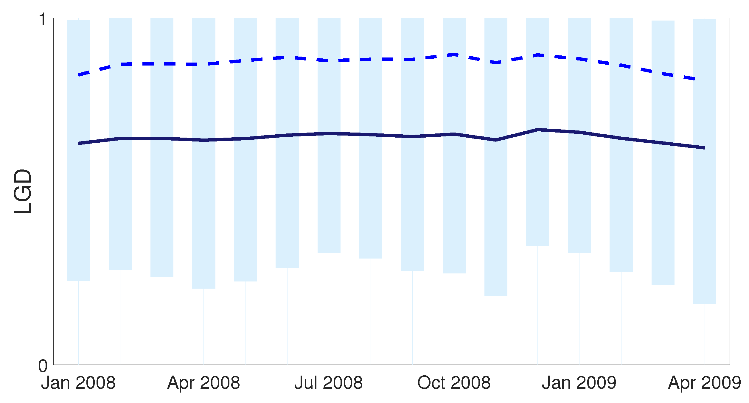
Figure 2.
Proportion of LGD observations for each month at 1 (dark blue bar), 0 (light blue bar), and on the intervals and (medium blue bar with diamonds at ).
Figure 2.
Proportion of LGD observations for each month at 1 (dark blue bar), 0 (light blue bar), and on the intervals and (medium blue bar with diamonds at ).
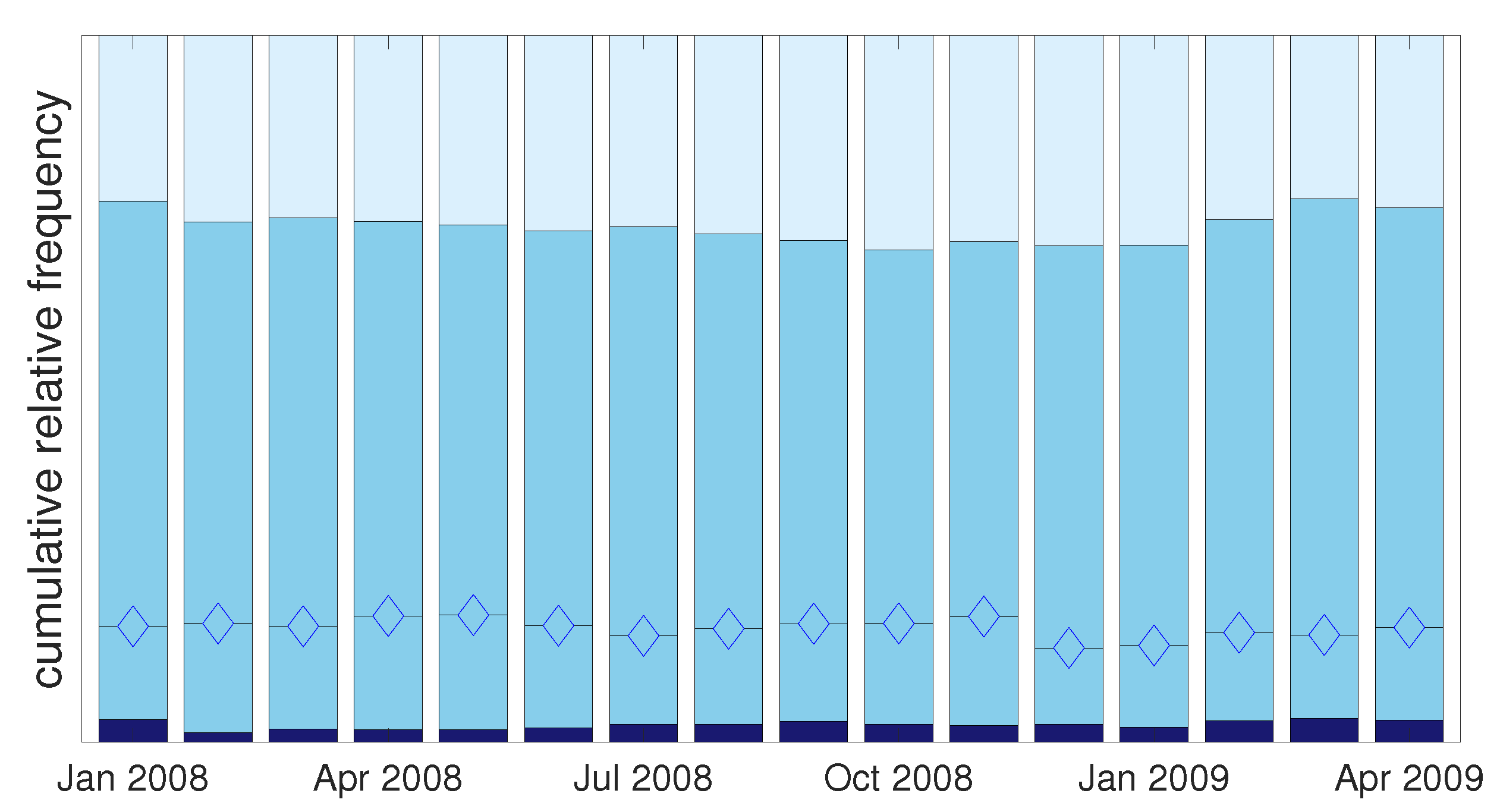
Figure 3.
The kernel density of the raw LGD data on (0, 1) compared to the fitted beta density for each month from January 2008 to April 2009.
Figure 3.
The kernel density of the raw LGD data on (0, 1) compared to the fitted beta density for each month from January 2008 to April 2009.
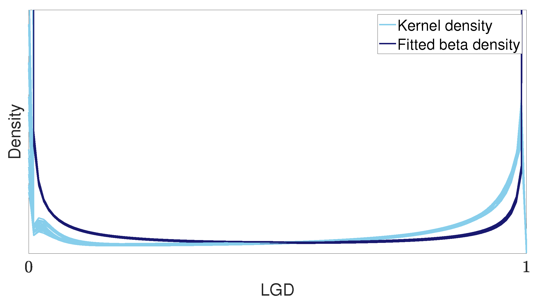
Figure 4.
Comparison of sample skewness for each month with that of the fitted beta distribution in the interval .
Figure 4.
Comparison of sample skewness for each month with that of the fitted beta distribution in the interval .
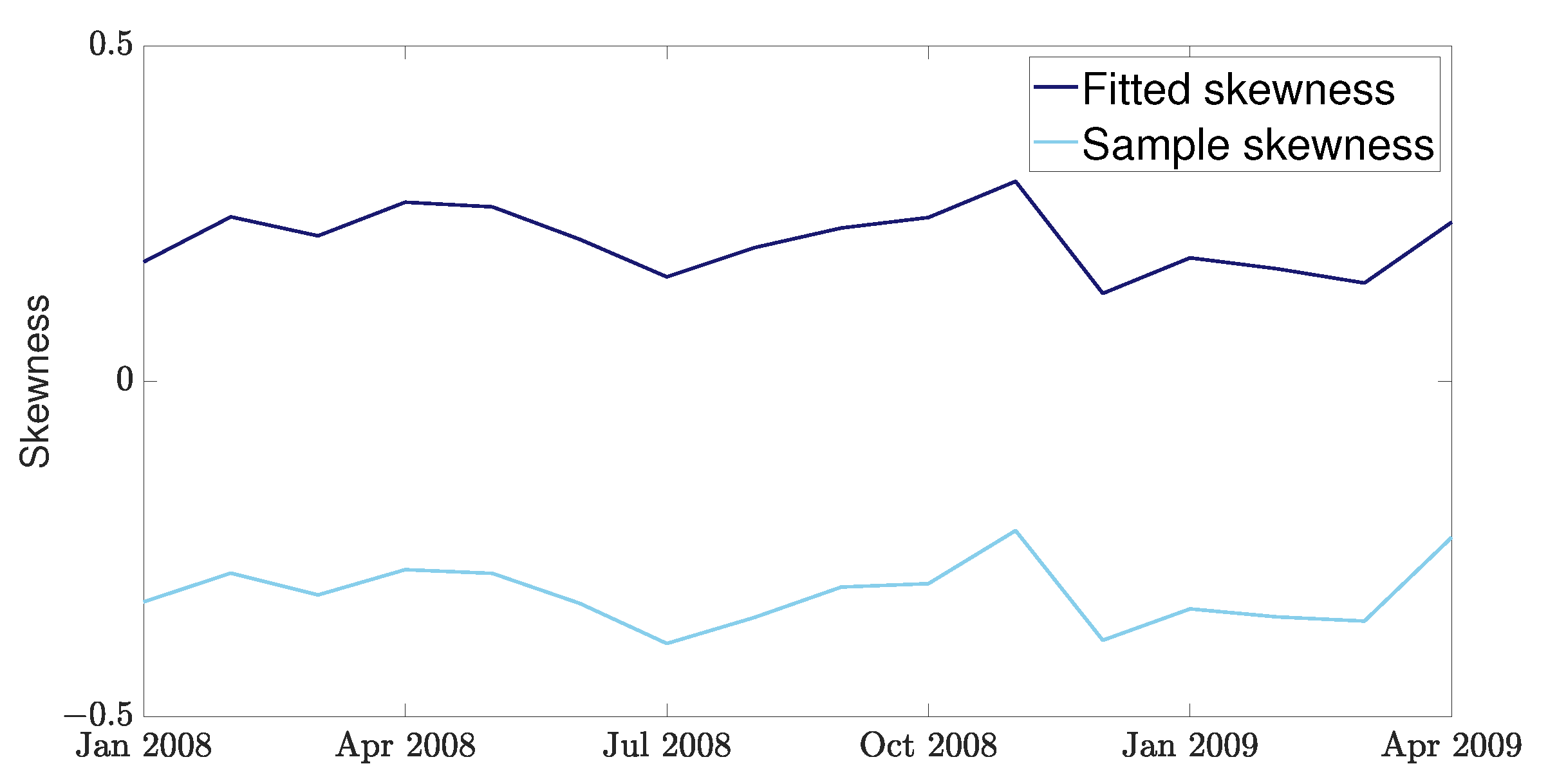
Figure 5.
The calculated empirical bias compared to the empirical bias after rounding for chosen values of .
Figure 5.
The calculated empirical bias compared to the empirical bias after rounding for chosen values of .

Figure 6.
The rate of change in the rounding bias plotted against the rounding threshold .
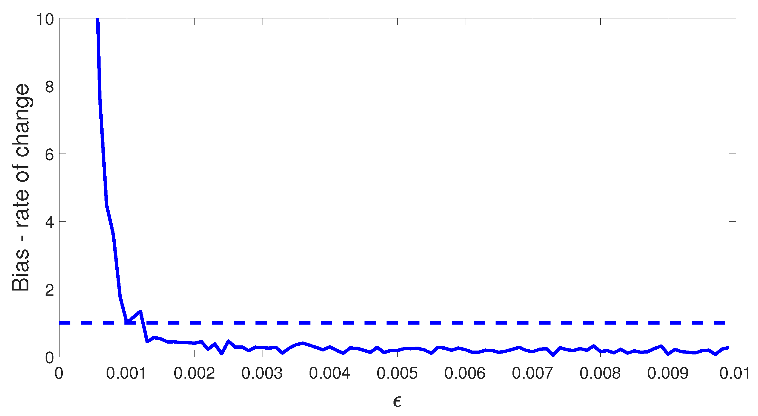
Figure 7.
The fitted mean of the beta and standard power distributions excluding observations between 0 and 1. The scale on the vertical axis is 0.1.
Figure 7.
The fitted mean of the beta and standard power distributions excluding observations between 0 and 1. The scale on the vertical axis is 0.1.
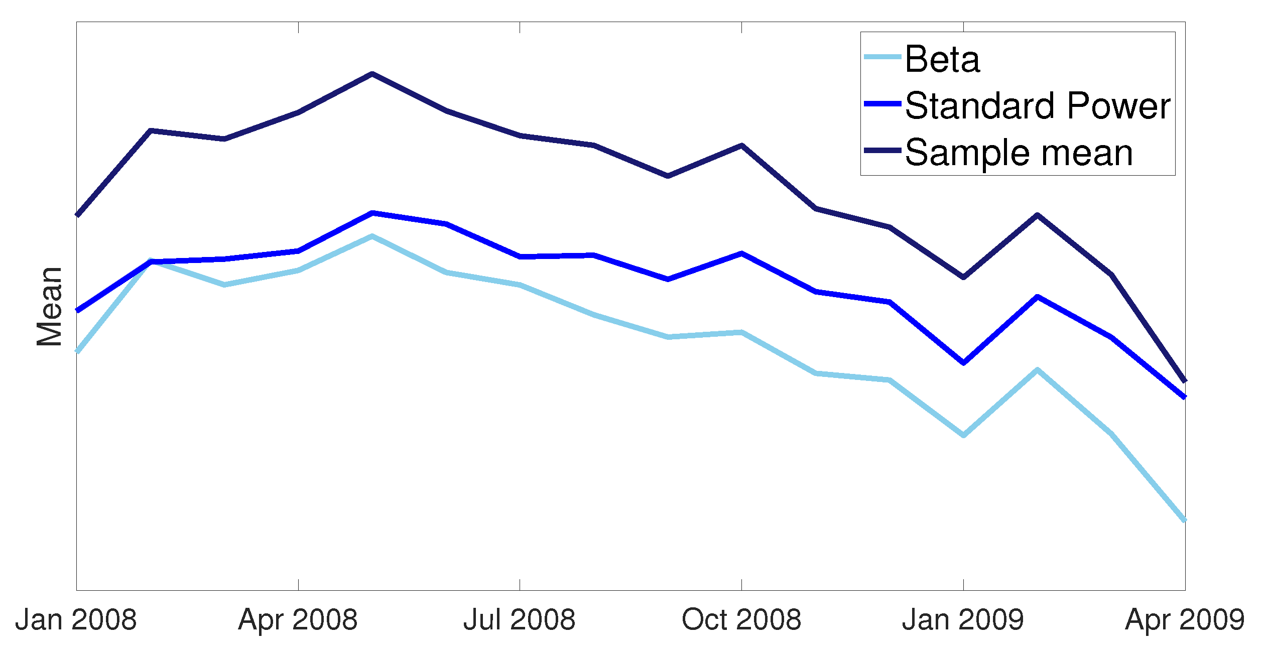
Figure 8.
QQ-plot of February 2008 LGD data against fitted beta distribution.

Figure 9.
Densities for February 2008 and March 2009 LGD data. On the left, the kernel density is compared to the fitted MSP model, while on the right, the two contributing SP fitted densities of the MSP model are shown, driven by and , respectively.
Figure 9.
Densities for February 2008 and March 2009 LGD data. On the left, the kernel density is compared to the fitted MSP model, while on the right, the two contributing SP fitted densities of the MSP model are shown, driven by and , respectively.
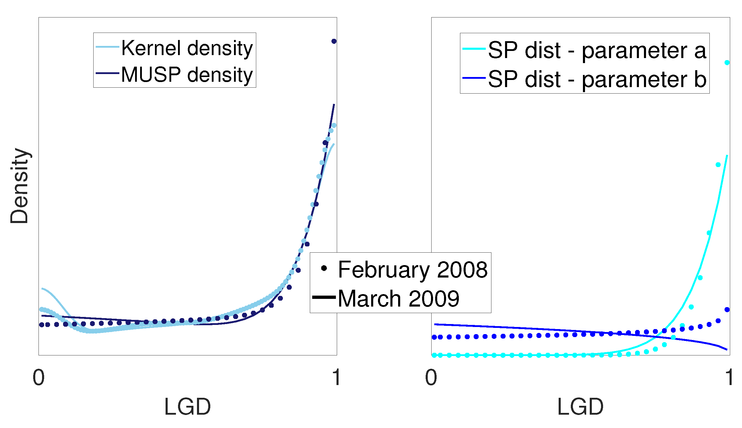
Figure 10.
The AIC of the ZOIB as well as ZOIMSP and ZOIMUSP models, plotted for each month.

Figure 11.
The empirical bias of the fitted ZOIMSP, ZOIMUSP, and benchmark ZOIB models plotted for each month.
Figure 11.
The empirical bias of the fitted ZOIMSP, ZOIMUSP, and benchmark ZOIB models plotted for each month.

Figure 12.
The bootstrap estimated mean of the AIC and BIC for ZOIB, ZOIMSP, and ZOIMUSP models for a sample size of . The shaded area represents a confidence interval for the mean of the ZOIMUSP model.
Figure 12.
The bootstrap estimated mean of the AIC and BIC for ZOIB, ZOIMSP, and ZOIMUSP models for a sample size of . The shaded area represents a confidence interval for the mean of the ZOIMUSP model.

Figure 13.
Bootstrap estimated mean of the AIC and BIC for the ZOIB, ZOIMSP, and ZOIMUSP models for a sample size of . The shaded area represents a confidence interval for the mean of the ZOIMUSP model.
Figure 13.
Bootstrap estimated mean of the AIC and BIC for the ZOIB, ZOIMSP, and ZOIMUSP models for a sample size of . The shaded area represents a confidence interval for the mean of the ZOIMUSP model.
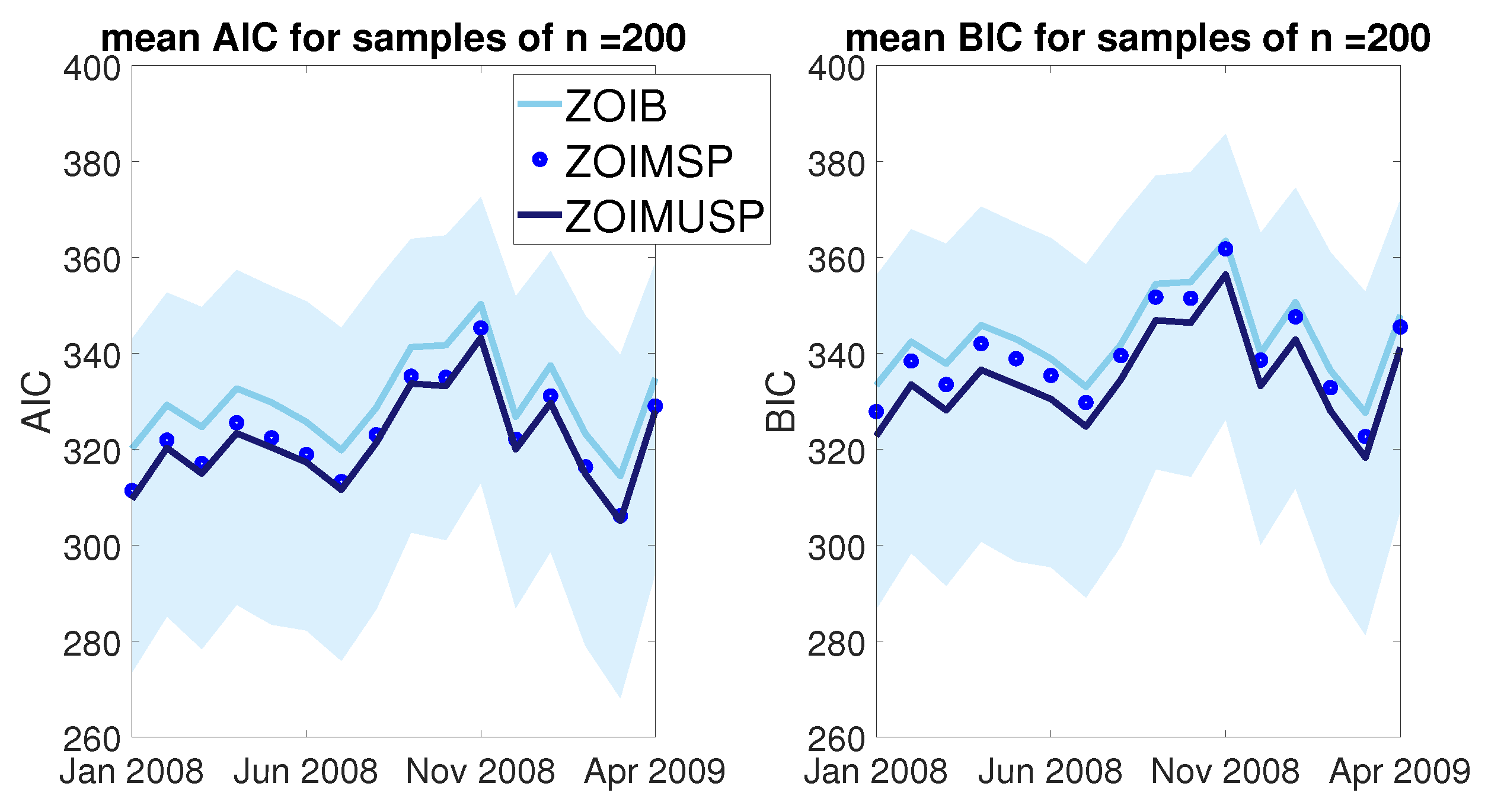
Figure 14.
Bootstrap estimated mean of the AIC and BIC for the ZOIB, ZOIMSP, and ZOIMUSP models for a sample size of . The shaded area represents a confidence interval for the mean of the ZOIMUSP model.
Figure 14.
Bootstrap estimated mean of the AIC and BIC for the ZOIB, ZOIMSP, and ZOIMUSP models for a sample size of . The shaded area represents a confidence interval for the mean of the ZOIMUSP model.

Figure 15.
Bootstrap estimates of the probability that the AIC (or BIC) for the fitted ZOIMSP and ZOIMUSP models is less than the AIC (or BIC) of the fitted ZOIB model over several months and for sample sizes of , and 500.
Figure 15.
Bootstrap estimates of the probability that the AIC (or BIC) for the fitted ZOIMSP and ZOIMUSP models is less than the AIC (or BIC) of the fitted ZOIB model over several months and for sample sizes of , and 500.


Table 1.
Parameter estimates of benchmark model.
| Bernoulli | Beta | |||
|---|---|---|---|---|
| Month | ||||
| 200801 | 0.266 | 0.881 | 0.303 | 0.653 |
| 200802 | 0.277 | 0.952 | 0.27 | 0.658 |
| 200803 | 0.276 | 0.934 | 0.277 | 0.646 |
| 200804 | 0.281 | 0.938 | 0.26 | 0.66 |
| 200805 | 0.286 | 0.939 | 0.255 | 0.643 |
| 200806 | 0.297 | 0.932 | 0.271 | 0.63 |
| 200807 | 0.296 | 0.916 | 0.298 | 0.626 |
| 200808 | 0.305 | 0.92 | 0.281 | 0.636 |
| 200809 | 0.319 | 0.908 | 0.277 | 0.655 |
| 200810 | 0.329 | 0.922 | 0.266 | 0.65 |
| 200811 | 0.316 | 0.925 | 0.256 | 0.682 |
| 200812 | 0.323 | 0.922 | 0.317 | 0.634 |
| 200901 | 0.318 | 0.933 | 0.311 | 0.672 |
| 200902 | 0.291 | 0.896 | 0.302 | 0.643 |
| 200903 | 0.265 | 0.872 | 0.319 | 0.651 |
| 200904 | 0.274 | 0.889 | 0.297 | 0.698 |
Table 2.
Parameter estimates with estimated standard errors in parenthesis of the ZOIB and ZOISP models on rounded LGD data.
Table 2.
Parameter estimates with estimated standard errors in parenthesis of the ZOIB and ZOISP models on rounded LGD data.
| Bernoulli | Beta | Standard Power | |||
|---|---|---|---|---|---|
| Month | |||||
| 200801 | 0.393 | 0.596 | 0.94 (0.019) | 0.525 (0.009) | 0.54 (0.008) |
| 200802 | 0.428 | 0.616 | 1.003 (0.02) | 0.521 (0.009) | 0.52 (0.007) |
| 200803 | 0.418 | 0.617 | 0.962 (0.02) | 0.51 (0.009) | 0.519 (0.008) |
| 200804 | 0.438 | 0.602 | 0.972 (0.021) | 0.509 (0.009) | 0.516 (0.008) |
| 200805 | 0.444 | 0.605 | 0.966 (0.021) | 0.493 (0.009) | 0.501 (0.008) |
| 200806 | 0.437 | 0.634 | 0.931 (0.019) | 0.488 (0.009) | 0.505 (0.018) |
| 200807 | 0.417 | 0.65 | 0.959 (0.018) | 0.508 (0.008) | 0.518 (0.007) |
| 200808 | 0.435 | 0.645 | 0.916 (0.018) | 0.496 (0.008) | 0.518 (0.007) |
| 200809 | 0.452 | 0.641 | 0.918 (0.019) | 0.506 (0.009) | 0.527 (0.008) |
| 200810 | 0.466 | 0.651 | 0.891 (0.018) | 0.489 (0.009) | 0.517 (0.008) |
| 200811 | 0.466 | 0.627 | 0.887 (0.019) | 0.503 (0.009) | 0.532 (0.008) |
| 200812 | 0.427 | 0.698 | 0.891 (0.018) | 0.508 (0.009) | 0.537 (0.008) |
| 200901 | 0.429 | 0.692 | 0.897 (0.016) | 0.533 (0.009) | 0.562 (0.008) |
| 200902 | 0.41 | 0.636 | 0.898 (0.016) | 0.507 (0.007) | 0.534 (0.007) |
| 200903 | 0.377 | 0.613 | 0.867 (0.014) | 0.514 (0.008) | 0.552 (0.006) |
| 200904 | 0.4 | 0.609 | 0.832 (0.014) | 0.527 (0.008) | 0.578 (0.007) |
Table 3.
Information criteria for the fitted ZOIB and ZOISP distributions.
| ZOIB | ZOISP | |||
|---|---|---|---|---|
| Month | AIC | BIC | AIC | BIC |
| 200801 | 13240 | 13268 | 13248 (0.06%) | 13269 (0.01%) |
| 200802 | 13418 | 13446 | 13416 (−0.01%) | 13437 (−0.07%) |
| 200803 | 12535 | 12563 | 12537 (0.02%) | 12558 (−0.04%) |
| 200804 | 12852 | 12880 | 12852 (0%) | 12873 (−0.05%) |
| 200805 | 13174 | 13202 | 13174 (0%) | 13195 (−0.05%) |
| 200806 | 12263 | 12291 | 12272 (0.07%) | 12293 (0.02%) |
| 200807 | 13817 | 13846 | 13820 (0.02%) | 13841 (−0.04%) |
| 200808 | 13900 | 13929 | 13918 (0.13%) | 13939 (0.07%) |
| 200809 | 14171 | 14199 | 14186 (0.11%) | 14207 (0.06%) |
| 200810 | 14699 | 14727 | 14730 (0.21%) | 14751 (0.16%) |
| 200811 | 15578 | 15606 | 15613 (0.22%) | 15634 (0.18%) |
| 200812 | 13102 | 13130 | 13133 (0.24%) | 13154 (0.18%) |
| 200901 | 15142 | 15170 | 15172 (0.2%) | 15194 (0.16%) |
| 200902 | 18403 | 18432 | 18443 (0.22%) | 18465 (0.18%) |
| 200903 | 17309 | 17338 | 17384 (0.43%) | 17406 (0.39%) |
| 200904 | 18401 | 18431 | 18526 (0.68%) | 18548 (0.63%) |
Table 4.
Parameter estimates with estimated standard errors in parenthesis for MSP and MUSP models.
| MSP | MUSP | ||||
|---|---|---|---|---|---|
| Month | |||||
| 200801 | 14.727 (0.722) | 0.892 (0.05) | 0.338 (0.02) | 13.618 (0.518) | 0.378 (0.007) |
| 200802 | 14.945 (0.753) | 0.798 (0.04) | 0.324 (0.02) | 13.047 (0.527) | 0.407 (0.007) |
| 200803 | 12.81 (0.601) | 0.879 (0.057) | 0.382 (0.023) | 11.983 (0.463) | 0.428 (0.008) |
| 200804 | 12.609 (0.615) | 0.82 (0.051) | 0.367 (0.024) | 11.575 (0.437) | 0.438 (0.008) |
| 200805 | 13.932 (0.676) | 0.769 (0.041) | 0.352 (0.021) | 12.447 (0.476) | 0.447 (0.008) |
| 200806 | 13.755 (0.717) | 0.739 (0.038) | 0.327 (0.021) | 12.329 (0.473) | 0.438 (0.008) |
| 200807 | 14.305 (0.726) | 0.768 (0.036) | 0.315 (0.019) | 12.466 (0.463) | 0.415 (0.007) |
| 200808 | 14.586 (0.747) | 0.761 (0.036) | 0.308 (0.02) | 12.522 (0.457) | 0.414 (0.007) |
| 200809 | 13.918 (0.713) | 0.816 (0.046) | 0.329 (0.022) | 12.318 (0.492) | 0.406 (0.008) |
| 200810 | 11.369 (0.561) | 1.041 (0.076) | 0.451 (0.024) | 11.522 (0.427) | 0.439 (0.008) |
| 200811 | 12.026 (0.581) | 0.974 (0.066) | 0.397 (0.023) | 11.827 (0.452) | 0.407 (0.008) |
| 200812 | 9.182 (0.439) | 1.411 (0.107) | 0.515 (0.02) | 11.651 (0.48) | 0.403 (0.008) |
| 200901 | 7.001 (0.415) | 1.873 (0.329) | 0.584 (0.063) | 10.77 (0.428) | 0.391 (0.008) |
| 200902 | 13.489 (0.551) | 0.911 (0.046) | 0.36 (0.019) | 12.641 (0.402) | 0.394 (0.006) |
| 200903 | 9.698 (0.392) | 1.375 (0.078) | 0.488 (0.015) | 12.241 (0.421) | 0.383 (0.006) |
| 200904 | 8.164 (0.32) | 1.708 (0.087) | 0.515 (0.012) | 12.455 (0.471) | 0.344 (0.007) |
Table 5.
Information criteria for the fitted ZOIMSP and ZOIMUSP models compared to the ZOIB model.
| ZOIB | ZOIMSP | ZOIMUSP | ||||
|---|---|---|---|---|---|---|
| Month | AIC | BIC | AIC | BIC | AIC | BIC |
| 200801 | 13240 | 13268 | 12822 (−3.2%) | 12858 (−3.1%) | 12825 (−3.1%) | 12853 (-3.1%) |
| 200802 | 13418 | 13446 | 13047 (−2.8%) | 13082 (−2.7%) | 13063 (−2.6%) | 13091 (−2.6%) |
| 200803 | 12535 | 12563 | 12156 (−3%) | 12190 (−3%) | 12155 (−3%) | 12183 (−3%) |
| 200804 | 12852 | 12880 | 12489 (−2.8%) | 12524 (−2.8%) | 12492 (−2.8%) | 12520 (−2.8%) |
| 200805 | 13174 | 13202 | 12791 (−2.9%) | 12826 (−2.8%) | 12801 (−2.8%) | 12829 (−2.8%) |
| 200806 | 12263 | 12291 | 11952 (−2.5%) | 11987 (−2.5%) | 11961 (−2.5%) | 11988 (−2.5%) |
| 200807 | 13817 | 13846 | 13458 (−2.6%) | 13494 (−2.5%) | 13476 (−2.5%) | 13505 (−2.5%) |
| 200808 | 13900 | 13929 | 13588 (−2.2%) | 13624 (−2.2%) | 13606 (−2.1%) | 13634 (−2.1%) |
| 200809 | 14171 | 14199 | 13852 (−2.2%) | 13887 (−2.2%) | 13858 (−2.2%) | 13887 (−2.2%) |
| 200810 | 14699 | 14727 | 14328 (−2.5%) | 14363 (−2.5%) | 14326 (−2.5%) | 14355 (−2.5%) |
| 200811 | 15578 | 15606 | 15269 (−2%) | 15304 (−1.9%) | 15267 (−2%) | 15295 (−2%) |
| 200812 | 13102 | 13130 | 12812 (−2.2%) | 12847 (−2.2%) | 12813 (−2.2%) | 12841 (−2.2%) |
| 200901 | 15142 | 15170 | 14717 (−2.8%) | 14753 (−2.8%) | 14735 (−2.7%) | 14763 (−2.7%) |
| 200902 | 18403 | 18432 | 17928 (−2.6%) | 17965 (−2.5%) | 17929 (−2.6%) | 17958 (−2.6%) |
| 200903 | 17309 | 17338 | 16779 (−3.1%) | 16816 (−3%) | 16787 (−3%) | 16817 (−3%) |
| 200904 | 18401 | 18431 | 18007 (−2.1%) | 18043 (−2.1%) | 18039 (−2%) | 18068 (−2%) |
Publisher’s Note: MDPI stays neutral with regard to jurisdictional claims in published maps and institutional affiliations. |
© 2022 by the authors. Licensee MDPI, Basel, Switzerland. This article is an open access article distributed under the terms and conditions of the Creative Commons Attribution (CC BY) license (https://creativecommons.org/licenses/by/4.0/).
Share and Cite
MDPI and ACS Style
Larney, J.; Grobler, G.L.; Allison, J.S. Introducing Two Parsimonious Standard Power Mixture Models for Bimodal Proportional Data with Application to Loss Given Default. Mathematics 2022, 10, 4520. https://doi.org/10.3390/math10234520
AMA Style
Larney J, Grobler GL, Allison JS. Introducing Two Parsimonious Standard Power Mixture Models for Bimodal Proportional Data with Application to Loss Given Default. Mathematics. 2022; 10(23):4520. https://doi.org/10.3390/math10234520
Chicago/Turabian StyleLarney, Janette, Gerrit Lodewicus Grobler, and James Samuel Allison. 2022. "Introducing Two Parsimonious Standard Power Mixture Models for Bimodal Proportional Data with Application to Loss Given Default" Mathematics 10, no. 23: 4520. https://doi.org/10.3390/math10234520
Note that from the first issue of 2016, this journal uses article numbers instead of page numbers. See further details here.