Prediction of Sea Level with Vertical Land Movement Correction Using Deep Learning

Abstract

Sea level rise (SLR) in small island countries such as Kiribati and Tuvalu have been a significant issue for decades. There is an urgent need for more accurate and reliable scientific information regarding SLR and its trend and for more informed decision making. This study uses the tide gauge (TG) dataset obtained from locations in Betio, Kiribati and Funafuti, Tuvalu with sea level corrections for vertical land movement (VLM) at these locations from the data obtained by the Global Navigation Satellite System (GNSS) before the sea level trend and rise predictions. The oceanic feature inputs of water temperature, barometric pressure, wind speed, wind gust, wind direction, air temperature, and three significant lags of sea level are considered in this study for data modeling. A new data decomposition method, namely, successive variational mode decomposition (SVMD), is employed to extract intrinsic modes of each feature that are processed for selection by the Boruta random optimizer (BRO). The study develops a deep learning model, namely, stacked bidirectional long short-term memory (BiLSTM), to make sea level (target variable) predictions that are benchmarked by three other AI models adaptive boosting regressor (AdaBoost), support vector regression (SVR), and multilinear regression (MLR). With a comprehensive evaluation of performance metrics, stacked BiLSTM attains superior results of 0.994207, 0.994079, 0.988219, and 0.899868 for correlation coefficient, Wilmott’s Index, the Nash–Sutcliffe Index, and the Legates–McCabe Index, respectively, for Kiribati, and with values of 0.996806, 0.996272, 0.992316, and 0.919732 for correlation coefficient, Wilmott’s Index, the Nash–Sutcliffe Index, and the Legates–McCabe Index, respectively, for the case of Tuvalu. It also shows the lowest error metrics in prediction for both study locations. Finally, trend analysis and linear projection are provided with the GNSS-VLM-corrected sea level average for the period 2001 to 2040. The analysis shows an average sea level rate rise of 2.1 mm/yr for Kiribati and 3.9 mm/yr for Tuvalu. It is estimated that Kiribati and Tuvalu will have a rise of 80 mm and 150 mm, respectively, by the year 2040 if estimated from year 2001 with the current trend.

1. Introduction

Sea level rise (SLR) is an important global issue and ranks among the top climate change issues, with international organizations concerned with the devastating impacts of climate change. The sixth assessment report of the Intergovernmental Panel on Climate Change (IPCC) [1,2] highlights that risks from SLR for coastal ecosystems and people are very likely to increase by tenfold if no adaptation and mitigation strategies are implemented as agreed by parties to the Paris agreement by the year 2100. The report further states that the global mean sea level (GMSL) has risen by 0.2 m since the year 1901 and is projected to rise further in the coming years. This also impacts the frequency of extreme sea levels, which are projected to increase by a median of 20–30 times across tide gauges by the year 2050 [2]. The global sea level rise (GSLR) rate has significantly increased from 1.7 mm/year to 3.4 mm/year since 1993 [3]. Sea level is a sensitive climate variable affected by various oceanic parameters. The rise in sea level has been attributed to the melting of glaciers and ice sheets, thereby adding water volume to the ocean [4]. The rate of melting has significantly increased over the past decade, and global warming has been stated as the major reason for this [3,5]. The impact of SLR could have devastating effects with a loss of 30–80% of coastal wetlands, which include salt marshes and mangroves [6]. A study on coastal hazard exposure of cultural, natural, and African heritage sites [7] found that by 2050, exposure to these areas will more than triple, reaching almost 200 sites as a result of climate change.

GSLR provides an estimate of the impact; however, the actual impact and rate of rise varies according to geographic location and other related climate variables. Miller and Douglas [8] stated the GSLR rate for the 20th Century to be between 1.5–2 mm/year, whereas Wadhams and Munk [9] found a lower rate of 1.1 mm/year in the same period of study. According to the IPCC report [10,11,12], small island nations are most vulnerable to SLR. Among these are South Pacific countries such as Kiribati and Tuvalu. Given the nature of these island states surrounded by oceans, SLR poses a major threat to their infrastructure and socioeconomic activities [12]. While the main aspect of SLR is highlighted as the inundation of coastal areas, the most critical and long term threat of impact will be on freshwater quality and availability [13]. The impacts of climate change on these island nations have been continuously highlighted in climate reports and media. However, as stated in [14], scientific knowledge and study in these islands have been relatively slow.

Sea level change is assessed by using three types of measurements, namely, tide gauge (TG) data, Global Navigation Satellite System (GNSS) time series, and observations of levelling [15,16]. TG provides a measure of sea level variation relative to a TG attached to a wharf. A problem associated with TG measurement is its inability to differentiate between sea level change and movement of the TG. In the case of land subsidence on which the tide gauge is situated, it records the relative sea level change [17]. In this study, tide gauge observations are corrected for land subsidence using the GNSS recorded measurements. GNSS measures the vertical crustal motion of the Earth with respect to the center of the Earth. Geoscience Australia (GA) operates the GNSS network, which includes the South Pacific countries, and provides this information under the Australian Aid-funded Pacific Sea Level and Geodetic Monitoring (PSLGM) Project. This technique has been successfully used in past studies for accurate sea level estimation. A study [18] using existing GNSS stations in Taiwan estimated the sea level change by removing vertical land motion (VLM) from the TG sea level measurement. Another study [19] claims that GNSS is able to provide VLM monitoring with an accuracy higher than 1 mm/year and hence is an effective tool to improve the estimation of sea level rise rates. VLM consideration in estimating accurate sea level rise is extremely important, as it removes a wide range of natural and anthropogenic influences from the tide gauge-measured sea level [16,20].

Furthermore, this study also addresses another important gap in study by utilizing new artificial intelligence (AI) methodologies, such as deep learning, to provide SLR trends and future localized projections for small islands such as Kiribati and Tuvalu in the South Pacific. The use of AI model predictions has been successfully carried out for various climate variables in many studies [21,22,23,24,25,26]. However, its implementation for the prediction of sea level with the VLM-corrected tide gauge dataset with data decomposition and feature selection techniques for South Pacific countries has not been considered so far. Therefore, this study proposes a deep learning architecture-based stacked bidirectional long short-term memory (BiLSTM) model as the objective model integrated with successive variational mode decomposition (SVMD) data decomposition and Boruta random forest optimizer feature selection for prediction of sea level. This is benchmarked by three AI models (adaptive boosting (AdaBoost) regressor, multilinear regression (MLR), and support vector regression (SVR). In addition, the corrected sea level average values are computed for a linear projection with the sea level rate rise for Kiribati and Tuvalu.

2. Materials and Methods

2.1. Study Area and Dataset

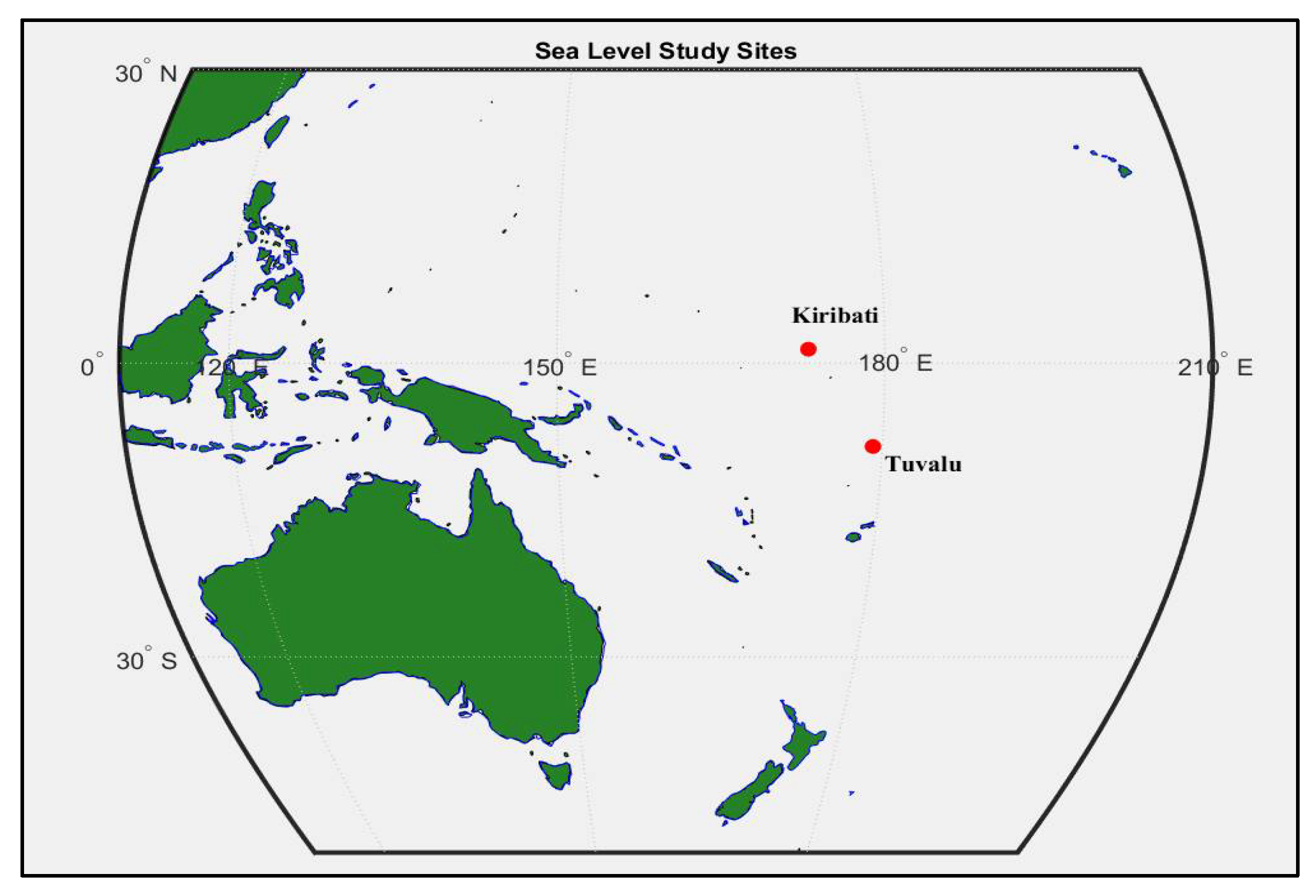
As mentioned previously, the two countries selected for this study are Kiribati and Tuvalu, located in the South Pacific Ocean. Figure 1 and

Table 1. Specific geographical location and description of the two data sites.

Country	Island/ Atoll	Town/ District	Seaframe Sensor Benchmark (SSBM)	Geographical Location
Kiribati	Tawara	Betio	4.6301	01°21′45″ N, 172°55′48″ E
Tuvalu	Funafuti	Fongafale	5.2468	08°30′10″ S, 179°12′33″ E

show the study area map and geographical locations of the two small island nations.

The study utilized a 60 min interval-recorded sea level (meters), water temperature (°C), air temperature (°C), barometric pressure (hPa), wind direction (degrees True), wind gust (m/s), and wind speed (m/s) dataset for the period of 2010–2021 acquired from the Bureau of Meteorology (BOM), Australia (Pacific Sea Level and Geodetic Monitoring Project File information and Instructions (bom.gov.au accessed on 10 February 2022)). The Pacific climate change data portal was developed with BOM under the Pacific Climate Change Science Program (PCCSP; 2009–2011). The sea level observations were recorded by the tide gauges deployed at the study sites mentioned in Table 1. The TG is one component of a water monitoring station and uses fitted sensors to collect measurements. Apart from sea level heights, the new technology is capable of measuring other oceanic parameters such as wind gusts and speed, air and water temperatures, and barometric pressure.

2.2. Data Preprocessing and Input Selection

An important aspect of any study based on data analysis is the quality of the data and scientific correctness of addressing the missing values [27]. This study used the interpolation method in Python using the Pandas library. The default status of linear was implemented, given the close relationship with the data points in the dataset. The effectiveness of machine learning modeling depends on this process, and deletion of rows is not an ideal option [28]. The next step was to confirm the stationarity of the dataset, which was done using the Augmented Dickey Fuller (ADF) test. ADF is used for large datasets and tests the null hypothesis on the presence of the unit root in the data. A larger negative value than the given critical value indicates that null hypothesis can be rejected. Hence, if no unit root is present, the dataset satisfies the stationarity criteria [29].

A time series dataset as used in this study is a collection of time ordered observations. Many studies [30,31,32,33] use lagged values as model inputs, as they help to reduce redundant features and improve the model prediction accuracy [34,35]. Figure 2 below shows the Auto Correlation Function (ACF) and the Partial Autocorrelation Function (PACF) plots of the sea level time series, which show the antecedent behavior of the lags for Kiribati. ACF shows the correlation of how any two values of the sea level series change as their separation changes. The ACF sinusoidal curve shows the seasonality and measures the association between current and past values, which will be useful in predicting future values in AI modelling [36]. The PACF analysis helps to show partial correlation of the series with its own lagged values. As shown in Figure 2, the line graph shows the level of correlation with each lag. Following the graph analysis for both time series (Kiribati and Tuvalu), three lags of sea level time series were chosen as inputs for the AI models.

The lags and all other oceanic parameters were tested for correlation, as shown in Figure 3. This correlation matrix calculates the correlation between each oceanic parameter with the sea level. The darker rectangle blocks show higher correlations between the parameters. Taking sea level as the target variable for prediction,

Table 2. Input features and description.

Input Oceanic Features
Air Temperature
Water Temperature
Wind Direction
Wind Gust
Wind Speed
Barometric Pressure
Sea Level Lags (t-1, t-2, t-3)

shows the input oceanic parameters and lagged values used for the AI models.

2.3. GNSS VLM Correction

The GNSS dataset is collected by Geoscience Australia (GA) using its infrastructure in Kiribati and Tuvalu. The three-dimensional GNSS position is computed every week with respect to the center of the Earth [37]. Figure 4 and Figure 5 show the graphs of GNSS and tide gauge variation from the average height. The tide gauge movement for absolute sea level analysis for Kiribati is provided as −3.4 ± 2.8 mm/year and Tuvalu as −1.5 ± 1.3 mm/year.

2.4. Data Normalization

All the model input and target data were normalized [38,39,40] for the values to be within [0,1] for modelling by Equation (1) below:

$$x_n=\frac{x_{\mathrm{actual}}-x_{\min }}{x_{\max }-x_{\min }}$$

(1)

After the modeling process, these values are computed to convert back to their original values. The $x_{\mathrm{actual}}$ in Equation (1) is made the subject, as shown in Equation (4).

$$x_{\mathrm{actual}}=x_n\left(x_{\max }-x_{\min }\right) +x_{\min }$$

(2)

where $x_n$ is the input dataset, $x_{\min }$ is the minimum value in the dataset, and $x_{\max }$ is the maximum value in the dataset.

2.5. Data Decomposition by Successive Variational Mode Decomposition (SVMD)

This study used successive variational mode decomposition (SVMD) proposed in [41], which successively extracts the modes without the need to know the number of modes. This new proposed method based on the same concept used in variational mode decomposition (VMD) decomposes the signal with lower computational complexity [41,42]. Variational mode extraction (VME) was applied successively on the input signal by adding constraints to negate convergence on the extracted modes in the previous step. This continued until all modes were extracted. To find a signal with the maximum compact spectrum L^th, an optimization problem is solved when this L^th mode reaches the extracted mode sum that reduces the reconstruction error. Figure 6 below shows the intrinsic mode decomposition (IMF) of Tuvalu sea level (lag) as an example of 500 data points. All input signals were decomposed into their IMFs for model inputs after Boruta feature selection, as used in many studies [43,44,45] to improve prediction accuracy.

2.6. Input Feature Selection Using Boruta Random Forest Optimizer (BRFO)

The algorithm of Boruta feature selection is based on the random forest classifier. The selection of the classifier is based on decision trees. The algorithm randomizes the input dataset, and duplicates are created as shadow attributes. The random forest classifier is then trained on the larger set using a feature importance measure to collect the z-scores. The maximum z-score is calculated within the shadow attributes, which form the critical values whereby attributes with higher than these values are included in the selected set. A statistical two-sided test of equality with attributes that had an undetermined importance is then performed. All the attributes with lower z-scores were removed from the set. Hence, all selected features were then ready for AI training and modeling for prediction [33,46,47].

2.7. Data Partition

There is no set rule for data partition; however, following past successful studies [23,48,49], the oceanic dataset was divided, as shown in

Table 3. The study data partition according to the timeline is shown in the table below.

Partition	Training (60%)	Validation (20%)	Testing (20%)
Oceanic Dataset	January 2000–December 2012	January 2013–June 2017	July 2017–December 2021

.

2.8. Objective Model Theoretical Background: Stacked Bidirectional Long Short-Term Memory (BiLSTM)

The LSTM-based models overcome a significant problem of RNNs of vanishing gradient and capture long term dependencies in the data modeling process. This deep learning architecture learns what information to preserve and what to remove. There are three gates (forget, input, and output), which handle the process, as shown in Figure 7.

The BiLSTM model extends the LSTM network in which each training sequence facilitates both forward and backward recurrent nets [33,50,51]. The input data passes through two LSTMs in this network model. The architecture uses full sequential information of all data points before with the movement through the layers [52,53]. There are two movements of input data, where data are first fed into the forward layer, and then the reverse form of input data are fed into the backward layer, as shown in Figure 8 [54]. The mathematical functions are given below for the units in the architecture:

Forget Gates:

$$f_t={\delta }_g\left(W_f{x}_t+U_f{h}_{t-1}+b_f\right)$$

(3)

Input Gates:

$$i_t={\delta }_g\left(W_i{x}_t+U_i{h}_{t-1}+b_i\right)$$

(4)

Output Gates:

$$o_t={\delta }_g\left(W_o{x}_t+U_o{h}_{t-1}+b_o\right)$$

(5)

Sigmoid Function:

$${\delta }_g\left(x\right)=\frac{1}{1+e^{-x}}$$

(6)

Cell Input State:

$$\check{c_t}=tanh\left(W_c{x}_t+U_c{h}_{t-1}+b_c\right)$$

(7)

Hypertangent Function:

$$tanh\left(x\right)=\frac{e^x-e^{-x}}{e^x+e^{-x}}$$

(8)

The $b_f$, $b_{i }$, $b_o$, and $b_c$play the role of bias vectors. The$U_f$,$U_i,$ $U_o,$ and $U_c$ are weight matrices that form the connection between the input cell state and the previous cell output state. $W_f,$ $W_i,$ $W_o,$ and $W_c$ are weight matrices of the forget gate. The network uses sigmoid (${\delta }_g$), which acts as the gate activation function [55]. The cell output $c_t$ and output $h_t$ are computed at each iteration $t$ as follows:

$$c_t=f_t\ast c_{t-1}+i_t\ast \check{c_t}$$

(9)

$$h_t=o_t\ast tanh(c_t)$$

(10)

Figure 8 shows how the data are processed in both directions with separate hidden layers. All the data input features go through BiLSTM layers in the network architecture. At the final stage, prediction output is given as $Y_t=[\dots y_{t-1}$,$y_t$,$y_{t+1}\dots ]$. The $y_t$value is found using the merge mode as:

$$y_t=\delta \left(\overrightarrow{h_t},\overleftarrow{h_t}\right)$$

(11)

2.9. Objective Model Development: Stacked Bidirectional Long Short-Term Memory (BiLSTM)

Model parameters are selected using a grid-search technique, which provides optimum values for the BiLSTM model. Figure 9 and

Table 4. The grid-search hyperparameter optimized parameters for BiLSTM modelling.

Optimizer	Activation Function	Weight Regularization	Dropout	Early Stopping
Adam	Rectified Linear Unit (ReLU)	L1 = 0, L2 = 0.01	0.1	Mode = Minimum, Patience = 20

show the tuning of parameters using grid-search and stacked BiLSTM deep learning architecture in Python during the modeling process.

2.10. Benchmark Models

The benchmark models have been widely used in predictions for many real-life applications. A robust ensemble method which combined random forest and gradient boosting to predict design routability and design rule checking (DRC) was used in [56]. In another study, ML algorithms are used to combine ensemble and heuristic greedy search methods for identifying design constraints and DRC [57]. SVR is regarded as an efficient ML model and shows high determination coefficients in [58] to predict evaporation amounts. One study [59] found high estimation results using MLR for the prediction of organic potato yield using tillage systems and soil properties. These models provide a sound comparative platform for the stacked BiLSTM model for the evaluation of performance in this study.

2.10.1. Support Vector Regression (SVR)

The support vector (SV) algorithm [60] based on non-linear generalization of the generalized portrait algorithm [60,61] was developed by Vapnik and co-workers. While it is generally used for classification, it can also be effectively applied for regression (SVR) problems. The regression version was also developed by Vapnik, Steven Golowich, and Alex Smola in 1997 [62]. The SVR algorithm uses a symmetrical loss function to train the dataset. The SVR computation complexity has the advantage of non-dependence on the dimensionality of the input space [63,64].

2.10.2. Adaptive Boosting Regressor (AdaBoost)

The adaptive boosting algorithm was first introduced by Freund and Schapire [65] in 1995. It is based on meta-estimation, where the dataset is fitted with a regressor. Following this, additional copies of the regressor is also fitted on the original dataset with an adjustment of the weights of instances with respect to predictor error [66].

2.10.3. Multilinear Regression (MLR)

Multilinear regression is a statistical technique, where many explanatory variables are used to predict a response variable [67]. It examines how multiple independent variables are related to a single dependent variable. The MLR assumptions are based on normal distribution, linearity, and freedom from extreme values, and observations are independent [68].

2.11. The Performance Evaluation Metrics for AI Models

All the models were evaluated using eight statistical metrics as given by Equations (12)–(19) on the testing dataset.

• Correlation Coefficient (r)

$$r={\left[\frac{{{\displaystyle \sum }}_{i=1}^n\left(D{O}_i-MDO\right)\left(D{S}_i-MDS\right)}{\sqrt{{{\displaystyle \sum }}_{i=1}^n{\left(D{O}_i-MDO\right)}^2{{\displaystyle \sum }}_{i=1}^n{\left(D{S}_i-MDS\right)}^2} }\right]}^2$$

(12)

2.

Willmott’s Index of Agreement (d)

$$d=1-\left[\frac{{{\displaystyle \sum }}_{i=1}^n{\left(D{O}_i-D{S}_i\right)}^2}{{{\displaystyle \sum }}_{i=1}^n{\left(\left|D{S}_i-MDO\left|+\right|D{O}_i-MDS\right|\right)}^2}\right]$$

(13)

3.

Nash–Sutcliffe Coefficient (NS)

$$NS=1-\left[\frac{{{\displaystyle \sum }}_{i=1}^n{\left(D{O}_i-D{S}_i\right)}^2}{{{\displaystyle \sum }}_{i=1}^n{\left(D{O}_i-MDO\right)}^2}\right],-\infty \le NS\le 1$$

(14)

4.

Legates and McCabe’s Index (LM)

$$LM=1-\left[\frac{{{\displaystyle \sum }}_{i=1}^n\left|\left(D{S}_i-D{O}_i\right)\right| }{{{\displaystyle \sum }}_{i=1}^n\left|D{O}_i-MDS\right|} \right], 0\le L\le 1$$

(15)

5.

Root Mean Square Error (RMSE)

$$RMSE=\sqrt{\frac{1}{n}{\displaystyle \sum }_{i=1}^n{\left(D{S}_i-D{O}_i\right)}^2}$$

(16)

6.

Mean Absolute Error (MABE)

$$MAE=\frac{1}{n}{\displaystyle \sum }_{i=1}^n\left|\left(D{S}_i-D{O}_i\right)\right|$$

(17)

7.

Relative Root Mean Square Error (RRMSE)

$$RRMSE=\frac{\sqrt{\left(\frac{1}{n}\right){{\displaystyle \sum }}_{i=1}^n{\left(D{S}_i-D{O}_i\right)}^2}}{\frac{1}{n}{{\displaystyle \sum }}_{i=1}^{n}D{O}_i}\times 100$$

(18)

8.

Mean Absolute Percentage Error (MAPE)

$$MAPE=\frac{1}{n} \left({\displaystyle \sum }_n^{i=1}\left|\frac{\left(D{S}_i-D{O}_i\right)}{D{O}_i} \right|\right)\times 100$$

(19)

where $D{S}_i$—simulated data, $D{O}_i$—observed data.

2.12. Schematic Diagram of the Data Analysis and Modelling

Figure 10 shows the steps involved in the preprocessing and VLM correction for absolute sea level. The initial block is critical for accurate and reliable results as key aspects of dataset preparation, such as the stationarity test, creation of lags, data normalization, and correlation analysis. Data decomposition into its intrinsic modes is an essential statistical step of the time series dataset, as it helps to extract features such as seasonality and trends. The Boruta random forest optimizer selects the significant features for the AI models. All preprocessed datasets are fed into the AI models, and the prediction output data are denormalized for conversion to actual sea level values.

3. Results

The preprocessed time series dataset with GNSS correction of VLM were divided into three sets, namely, training, validation, and testing. These were then put into the AI models as feature inputs and target variables. The prediction model was developed in each case for sea level prediction. The evaluation was divided in two parts, firstly, the efficiency metrics measuring the accuracy of the models, and secondly, error metrics for predicted values. The correlation coefficient (r) is a widely used statistical measure that determines the relationship between two variables [69]. It indicates the strength of association, and in this case, the degree of association between the observed and predicted sea level values for all models. Wilmott’s Index [70] is a standardized dimensionless measure that indicates the ratio of the mean of square error and the potential error. It detects the additive and proportional differences in the means and variances between observed and predicted values [70,71]. Nash–Sutcliffe (NS) [72] is a normalized metric that provides model accuracy with goodness of fit [73,74]. The index uses three quantities, namely, measured values, means of measured values, and the predicted values [73]. The Legates and McCabe Index [75] is considered to be a more advanced and efficient statistical index, where the adjustment of comparisons in the evaluation of WI is utilized [76]. There are four error metrics utilized for analyses of all models at both study sites, namely, root mean square error (RMSE), mean absolute error (MABE), relative root mean square error (RRMSE), and mean absolute percentage error (MAPE).

3.1. Objective and Benchmark Model Results for Kiribati and Tuvalu

The model performance and error metrics are shown in

Table 5. Model performance metrics for Kiribati.

Model	Correlation Coefficient (r)	Willmott’s Index of Agreement (d)	Nash–Sutcliffe Coefficient (NS)	Legates and McCabe Index (L)
AdaBoost	0.964311	0.957647	0.923809	0.733546
MLR	0.758946	0.672739	0.368981	0.217703
SVR	0.988909	0.987155	0.974866	0.852321
BiLSTM	0.994207	0.994079	0.988219	0.899868

,

Table 6. Model error metrics for Kiribati.

Model	RMSE	MABE	RRMSE	MAPE
AdaBoost	0.137814	0.111508	7.990359	7.322568
MLR	0.396610	0.327382	22.995112	21.019548
SVR	0.079154	0.061802	4.589257	3.889261
BiLSTM	0.054191	0.041904	3.141943	2.672222

,

Table 7. Model performance metrics for Tuvalu.

Model	Correlation Coefficient (r)	Willmott’s Index of Agreement (d)	Nash–Sutcliffe Coefficient (NS)	Legates and McCabe Index (L)
AdaBoost	0.963663	0.959991	0.925800	0.744654
MLR	0.967652	0.908565	0.822057	0.592441
SVR	0.981239	0.979752	0.960339	0.807352
BiLSTM	0.996806	0.996272	0.992316	0.919732

and

Table 8. Model error metrics for Tuvalu.

Model	RMSE	MABE	RRMSE	MAPE
AdaBoost	0.127630	0.101366	6.061497	4.998458
MLR	0.197646	0.161790	9.386780	7.673520
SVR	0.093310	0.076476	4.431582	3.759054
BiLSTM	0.041071	0.031864	1.950591	1.625925

.

3.2. Scatterplot with Correlation and Histogram Error Results for Kiribati and Tuvalu Models

A scatterplot is considered as one of the most powerful data analysis tools [77]. It is a plot of two variables (observed and predicted) to show the association between them. This technique emerged with the need to examine bivariate relationships between separate variables directly [78]. The linear regression fit with a coefficient of determination (r²) further adds to more information on the scatterplot about the behavior between the variables in the study [79]. The stacked BiLSTM as the objective model for this study, as shown in Figure 11, shows more compactness in the scatter of points between observed and predicted values, indicating that higher accuracy and higher r² further supports this graphical representation. The MLR plot shows wider scattering with the lowest r² value, indicating lower model accuracy.

A histogram is another widely used and common display chart in scientific study and coined by famous statistician Karl Pearson [80]. It is constructed using attributes (absolute prediction error) by partitioning the data distribution into "buckets" or "bins" with their frequency in the allocated ranges [80,81]. It is an effective graphical method to evaluate the performance of model prediction, as it shows the frequency of prediction error and its distribution within the "bins". The stacked BiLSTM model plot in Figure 12 shows the bars in the lower bracket indicating lesser amounts of absolute prediction error. On the contrary, other benchmark models in Figure 11 have more bars extending to the right, indicating higher absolute prediction error.

4. Discussion

4.1. Objective and Benchmark Model Performance Evaluation

As shown in Figure 13, all efficiency metrics discussed previously show superior performance by the stacked BiLSTM model for both study sites. It attains high performance values of 0.994207, 0.994079, 0.988219, and 0.899868 for the correlation coefficient, Wilmott’s Index, the Nash–Sutcliffe Index, and the Legates–McCabe Index, respectively, for Kiribati. The SVR model has also performed well as a benchmark model attaining values of 0.988909, 0.987155, 0.974866, and 0.852321 for the correlation coefficient, Wilmott’s Index, the Nash–Sutcliffe Index, and the Legates–McCabe Index, respectively. MLR performed very poorly at both study locations with values of 0.758946, 0.672739, 0.368981, and 0.217703 for Kiribati. Compared with other models, this is also similar for Tuvalu, as shown in Figure 14 but with better performance values of 0.967652, 0.908565, 0.822057, and 0.592441 for the correlation coefficient, Wilmott’s Index, the Nash–Sutcliffe Index, and the Legates–McCabe Index, respectively. Stacked BiLSTM has also shown superior results for Tuvalu with values of 0.996806, 0.996272, 0.992316, and 0.919732. AdaBoost as a benchmark model has also shown good performance for both study sites, attaining values of 0.137814, 0.111508, 7.990359, and 7.322568 for Kiribati and 0.963663, 0.959991, 0.925800, and 0.744654 for Tuvalu.

4.2. Objective and Benchmark Model Error Evaluation

To support the performance metrics above, error calculations were done for each model with their prediction results. Error evaluation is a significant aspect of model evaluation, as shown in many past studies using AI models for prediction [33,45]. Four error metrics are computed in this study for error analysis. Figure 15 and Figure 16 show the bar charts for model errors at both study sites. It is clearly evident that the stacked BiLSTM model outperformed all other models with the lowest values of 0.041071, 0.031864, 1.950591, and 1.625925 for root mean square error (RMSE), mean absolute error (MABE), relative root mean square error (RRMSE), and mean absolute percentage error (MAPE), respectively. This is similar for Tuvalu with values of 0.041071, 0.031864, 1.950591, and 1.625925 in the same order. MLR had the highest error values in both cases with 0.396610, 0.327382, 22.995112, and 21.019548 (Kiribati) and 0.197646, 0.161790, 9.386780, and 7.673520 (Tuvalu) for root mean square error (RMSE), mean absolute error (MABE), relative root mean square error (RRMSE), and mean absolute percentage error (MAPE), respectively.

4.3. Times Series Comparison of Models for Kiribati and Tuvalu Sea Levels

Figure 17 shows a time series comparison of all model results between 23 December 2021 and 31 December 2021. The data points show the tracking of observed and predicted data points within the testing phase of modeling. All AI models are able to track the observed data; however, stacked BiLSTM shows the best fit, and all predicted points overlap, indicating greater accuracy than all benchmark models. The MLR model shows most deviation between the observed and predicted points. AdaBoost and SVR also show better tracking of the GNSS-VLM sea level than the MLR model with the predicted dataset.

4.4. GNSS-VLM-Corrected Sea Level Trend Analysis and Linear Projection

Figure 18 shows the annual sea level average with VLM correction with 2 per moving average, which shows an increasing trend based on the analysis of the tide gauge dataset located in Tarawa, Kiribati. The GNSS-VLM measurement was adjusted from each observation for the analysis. The annual rate of increase is estimated to be 2.1 mm/year, and with a linear projection, the sea level is expected to reach close to 1.75 m in 2040. This is an estimated increase from 1.67 m at an average of 80 mm. According to [82], there is a significant increase in the extreme water level according to Betio tide gauge data since 1984 (>2.8 m above datum) due to decadal variability in the frequency of “Central Pacific” El Niño events. Furthermore, it states that sea level variability could increase by 20–40 mm by the end of century due to the evolution of ENSO dynamics and including other factors. In another study of Tarawa in Kiribati [83], a sea level rise rate trend of 3.9 mm per year was found from 1992 to 2008.

Figure 19 shows the annual average GNSS-VLM-corrected sea level trend for Tuvalu. The rate of rise is higher in the case of Tuvalu, with an annual average rate rise of 3.9 m/year. The linear projection shows an estimate rise to 2.16 m for 2040 with an increase of 150 mm from 2.01 m. Other studies, such as Donner and Webber [84], of sea level rise in Tuvalu, with a 16-year TG data analysis from 2008, found a higher average rate rise of 5.9 mm/year. The higher values can be attributed to a different timeline considered as this study considers the dataset from 2001 to 2021 and the consideration of GNSS-VLM TG adjustment in sea level observations.

5. Conclusions

Based on the implementation of artificial intelligence models, including new deep learning analysis with data decomposition, it can be clearly seen with the comprehensive evaluation of all AI models shown that the GNSS-VLM-corrected sea level trend can be predicted with high accuracy. The objective stacked BiLSTM model outperformed all benchmark models in the study with greater accuracy. The trend assessment and linear forecast with the new GNSS-VLM-corrected average values provides insight into the highly debated issue of sea level rise with climate change in small island countries. With use of a recent dataset and improved accuracy of predicted rise, stakeholders can make better decisions on adaptation and mitigation strategies for Kiribati and Tuvalu. There is no doubt that the sea level is rising and that the extent and nature of its impact is different across the world. As seen in the analysis of this study, the expected rate of rise in Kiribati (2.1 mm/year) is not the same as in Tuvalu (3.9 mm/year) despite being in the South Pacific region. This information needs to be considered with other factors such as the topological changes in the land area to assess how the impacts may occur on the atoll islands with their vulnerability to flooding and inundation. Each island state has its own context of geographic, topographic, and cultural variety which must be assessed for real impacts of sea level rise [85]. This can be a future scope for the extension of this study.

References

- Pörtner, H.-O.; Roberts, D.C.; Adams, H.; Adler, C.; Aldunce, P.; Ali, E.; Begum, R.A.; Betts, R.; Kerr, R.B.; Biesbroek, R.; et al. Climate Change 2022: Impacts, Adaptation, and Vulnerability. Contribution of Working Group II to the Sixth Assessment Report of the Intergovernmental Panel on Climate Change; IPCC: Geneva, Switzerland, 2022. [Google Scholar]
- Cooley, S.; Schoeman, D.; Bopp, L.; Boyd, P.; Donner, S.; Ito, S.-I.; Kiessling, W.; Martinetto, P.; Ojea, E.; Racault, M.-F.; et al. Oceans and Coastal Ecosystems and Their Services. In IPCC AR6 WGII; Cambridge University Press: Cambridge, UK, 2022. [Google Scholar]
- Lindsey, R. Climate Change: Global Sea Level. Available online: Climate.gov (accessed on 14 August 2020).
- Braddock, S.; Hall, B.L.; Johnson, J.S.; Balco, G.; Spoth, M.; Whitehouse, P.L.; Campbell, S.; Goehring, B.M.; Rood, D.H.; Woodward, J. Relative sea-level data preclude major late Holocene ice-mass change in Pine Island Bay. Nat. Geosci. 2022, 15, 568–572. [Google Scholar] [CrossRef]
- Meehl, G.A.; Washington, W.M.; Collins, W.D.; Arblaster, J.M.; Hu, A.; Buja, L.E.; Strand, W.G.; Teng, H. How much more global warming and sea level rise? Science 2005, 307, 1769–1772. [Google Scholar] [CrossRef] [PubMed] [Green Version]
- Van Dobben, H.F.; De Groot, A.V.; Bakker, J.P. Salt marsh accretion with and without deep soil subsidence as a proxy for sea-level rise. Estuaries Coasts 2022, 45, 1562–1582. [Google Scholar] [CrossRef]
- Vousdoukas, M.I.; Clarke, J.; Ranasinghe, R.; Reimann, L.; Khalaf, N.; Duong, T.M.; Ouweneel, B.; Sabour, S.; Iles, C.E.; Trisos, C.H.; et al. African heritage sites threatened as sea-level rise accelerates. Nat. Clim. Change 2022, 12, 256–262. [Google Scholar] [CrossRef]
- Miller, L.; Douglas, B.C. Mass and volume contributions to twentieth-century global sea level rise. Nature 2004, 428, 406–409. [Google Scholar] [CrossRef] [PubMed] [Green Version]
- Wadhams, P.; Munk, W. Ocean freshening, sea level rising, sea ice melting. Geophys. Res. Lett. 2004, 31. [Google Scholar] [CrossRef] [Green Version]
- Watson, T.R.; Zinyowera, M.C.; Moss, R.H. Climate Change 1995. Impacts, Adaptations and Mitigation of Climate Change: Scientific-Technical Analyses; Cambridge University Press: Cambridge, UK, 1996. [Google Scholar]
- Githeko, A.K.; Woodward, A. International consensus on the science of climate and health: The IPCC Third Assessment Report. In Climate Change and Human Health: Risks and Responses; World Health Organization: Geneva, Switzerland, 2003; pp. 43–60. [Google Scholar]
- Nurse, L.A.; Sem, G.; Hay, J.E.; Suarez, A.G.; Wong, P.P.; Briguglio, L.; Ragoonaden, S. Small island states. In Climate Change; Cambridge University Press: Cambridge, UK, 2001; pp. 843–875. [Google Scholar]
- Burns, W.C. The Impact of Climate Change on Pacific Island Developing Countries in the 21st Century. In Climate Change in the South Pacific: Impacts and Responses in Australia, New Zealand, and Small Island States; Springer: Berlin/Heidelberg, Germany, 2000; pp. 233–250. [Google Scholar]
- Campbell, J.; Barnett, J. Climate Change and Small Island States: Power, Knowledge and the South Pacific; Routledge: Oxfordshire, UK, 2010. [Google Scholar]
- Santamaría-Gómez, A.; Watson, C.; Gravelle, M.; King, M.; Wöppelmann, G. Levelling co-located GNSS and tide gauge stations using GNSS reflectometry. J. Geod. 2015, 89, 241–258. [Google Scholar] [CrossRef]
- Wöppelmann, G.; Marcos, M. Vertical land motion as a key to understanding sea level change and variability. Rev. Geophys. 2016, 54, 64–92. [Google Scholar] [CrossRef] [Green Version]
- Blewitt, G.; Altamimi, Z.; Davis, J.; Gross, R.; Kuo, C.-Y.; Lemoine, F.G.; Moore, A.W.; Neilan, R.E.; Plag, H.-P.; Rothacher, M. Geodetic observations and global reference frame contributions to understanding sea-level rise and variability. In Understanding Sea-Level Rise and Variability; Blackwell Publishing Ltd.: Hoboken, NJ, USA, 2010; pp. 256–284. [Google Scholar]
- Lee, C.-M.; Kuo, C.-Y.; Sun, J.; Tseng, T.-P.; Chen, K.-H.; Lan, W.-H.; Shum, C.; Ali, T.; Ching, K.-E.; Chu, P. Evaluation and improvement of coastal GNSS reflectometry sea level variations from existing GNSS stations in Taiwan. Adv. Space Res. 2019, 63, 1280–1288. [Google Scholar] [CrossRef]
- Dawidowicz, K. Sea level changes monitoring using GNSS technology–A review of recent efforts. Acta Adriat. Int. J. Mar. Sci. 2014, 55, 145–161. [Google Scholar]
- Anzidei, M.; Antonioli, F.; Benini, A.; Lambeck, K.; Sivan, D.; Serpelloni, E.; Stocchi, P. Sea level change and vertical land movements since the last two millennia along the coasts of southwestern Turkey and Israel. Quat. Int. 2011, 232, 13–20. [Google Scholar] [CrossRef]
- Ghimire, S.; Deo, R.C.; Downs, N.J.; Raj, N. Global solar radiation prediction by ANN integrated with European Centre for medium range weather forecast fields in solar rich cities of Queensland Australia. J. Clean. Prod. 2019, 216, 288–310. [Google Scholar] [CrossRef]
- Ghimire, S.; Deo, R.C.; Raj, N.; Mi, J. Wavelet-based 3-phase hybrid SVR model trained with satellite-derived predictors, particle swarm optimization and maximum overlap discrete wavelet transform for solar radiation prediction. Renew. Sustain. Energy Rev. 2019, 113, 109247. [Google Scholar] [CrossRef]
- Neupane, A.; Raj, N.; Deo, R.; Ali, M. Development of data-driven models for wind speed forecasting in Australia. In Predictive Modelling for Energy Management and Power Systems Engineering; Elsevier: Amsterdam, The Netherlands, 2021; pp. 143–190. [Google Scholar]
- Ahmed, A.M.; Deo, R.C.; Raj, N.; Ghahramani, A.; Feng, Q.; Yin, Z.; Yang, L. Deep learning forecasts of soil moisture: Convolutional neural network and gated recurrent unit models coupled with satellite-derived MODIS, observations and synoptic-scale climate index data. Remote Sens. 2021, 13, 554. [Google Scholar] [CrossRef]
- Liu, Y.; Li, D.; Wan, S.; Wang, F.; Dou, W.; Xu, X.; Li, S.; Ma, R.; Qi, L. A long short-term memory-based model for greenhouse climate prediction. Int. J. Intell. Syst. 2022, 37, 135–151. [Google Scholar] [CrossRef]
- Tsekouras, G.E.; Trygonis, V.; Maniatopoulos, A.; Rigos, A.; Chatzipavlis, A.; Tsimikas, J.; Mitianoudis, N.; Velegrakis, A.F. A Hermite neural network incorporating artificial bee colony optimization to model shoreline realignment at a reef-fronted beach. Neurocomputing 2018, 280, 32–45. [Google Scholar] [CrossRef]
- Rahm, E.; Do, H.H. Data cleaning: Problems and current approaches. IEEE Data Eng. Bull. 2000, 23, 3–13. [Google Scholar]
- Brownlee, J. Data Preparation for Machine Learning: Data Cleaning, Feature Selection, and Data Transforms in Python; Machine Learning Mastery: San Juan, Puerto Rico, 2020. [Google Scholar]
- Mushtaq, R. Augmented dickey fuller test. SSRN Electron. J. 2011. [Google Scholar] [CrossRef]
- Ghimire, S.; Deo, R.C.; Raj, N.; Mi, J. Deep solar radiation forecasting with convolutional neural network and long short-term memory network algorithms. Appl. Energy 2019, 253, 113541. [Google Scholar] [CrossRef]
- Sharma, E.; Deo, R.C.; Soar, J.; Prasad, R.; Parisi, A.V.; Raj, N. Novel hybrid deep learning model for satellite based PM10 forecasting in the most polluted Australian hotspots. Atmos. Environ. 2022, 279, 119111. [Google Scholar] [CrossRef]
- Mouatadid, S.; Raj, N.; Deo, R.C.; Adamowski, J.F. Input selection and data-driven model performance optimization to predict the Standardized Precipitation and Evaporation Index in a drought-prone region. Atmos. Res. 2018, 212, 130–149. [Google Scholar] [CrossRef]
- Raj, N.; Brown, J. An EEMD-BiLSTM Algorithm Integrated with Boruta Random Forest Optimiser for Significant Wave Height Forecasting along Coastal Areas of Queensland, Australia. Remote Sens. 2021, 13, 1456. [Google Scholar] [CrossRef]
- Ribeiro, G.H.; Neto, P.S.d.M.; Cavalcanti, G.D.; Tsang, R. Lag selection for time series forecasting using particle swarm optimization. In The 2011 International Joint Conference on Neural Networks; IEEE: Manhattan, NY, USA, 2011. [Google Scholar]
- Muttil, N.; Chau, K.-W. Machine-learning paradigms for selecting ecologically significant input variables. Eng. Appl. Artif. Intell. 2007, 20, 735–744. [Google Scholar] [CrossRef] [Green Version]
- Flores, F.J.H.; Engel, P.M.; Pinto, R.C. Autocorrelation and partial autocorrelation functions to improve neural networks models on univariate time series forecasting. In The 2012 International Joint Conference on Neural Networks (IJCNN); IEEE: Manhattan, NY, USA, 2012. [Google Scholar]
- Jia, M. The South Pacific Sea Level & Climate Monitoring Project; Australian Government, Bureau of Meteorology: Melbourne Docklands, VIC, Australia, 2011.
- Kotsiantis, S.; Kanellopoulos, D.; Pintelas, P. Data preprocessing for supervised leaning. Int. J. Comput. Sci. 2006, 1, 111–117. [Google Scholar]
- Deo, R.C.; Ghimire, S.; Downs, N.J.; Raj, N. Optimization of windspeed prediction using an artificial neural network compared with a genetic programming model. In Handbook of Research on Predictive Modeling and Optimization Methods in Science and Engineering; IGI Global: Hershey, PA, USA, 2018; pp. 328–359. [Google Scholar]
- Ghimire, S.; Deo, R.C.; Downs, N.J.; Raj, N. Self-adaptive differential evolutionary extreme learning machines for long-term solar radiation prediction with remotely-sensed MODIS satellite and Reanalysis atmospheric products in solar-rich cities. Remote Sens. Environ. 2018, 212, 176–198. [Google Scholar] [CrossRef]
- Nazari, M.; Sakhaei, S.M. Successive variational mode decomposition. Signal Process. 2020, 174, 107610. [Google Scholar] [CrossRef]
- Wang, X.; Ma, J. Weak Fault Feature Extraction of Rolling Bearing Based on SVMD and Improved MOMEDA. Math. Probl. Eng. 2021, 2021, 9966078. [Google Scholar] [CrossRef]
- Peng, T.; Zhou, J.; Zhang, C.; Zheng, Y. Multi-step ahead wind speed forecasting using a hybrid model based on two-stage decomposition technique and AdaBoost-extreme learning machine. Energy Convers. Manag. 2017, 153, 589–602. [Google Scholar] [CrossRef]
- Da Silva, R.G.; Ribeiro, M.H.D.M.; Mariani, V.C.; dos Santos Coelho, L. Forecasting Brazilian and American COVID-19 cases based on artificial intelligence coupled with climatic exogenous variables. Chaos Solitons Fractals 2020, 139, 110027. [Google Scholar] [CrossRef]
- Raj, N.; Gharineiat, Z.; Ahmed, A.A.M.; Stepanyants, Y. Assessment and Prediction of Sea Level Trend in the South Pacific Region. Remote Sens. 2022, 14, 986. [Google Scholar] [CrossRef]
- Kursa, M.B.; Rudnicki, W.R. Feature selection with the Boruta package. J. Stat. Softw. 2010, 36, 1–13. [Google Scholar] [CrossRef] [Green Version]
- Kotsiantis, S.B. Decision trees: A recent overview. Artif. Intell. Rev. 2013, 39, 261–283. [Google Scholar] [CrossRef]
- Deo, C.R.; Samui, P.; Kim, D. Estimation of monthly evaporative loss using relevance vector machine, extreme learning machine and multivariate adaptive regression spline models. Stoch. Environ. Res. Risk Assess. 2016, 30, 1769–1784. [Google Scholar] [CrossRef]
- Deo, R.C.; Ghorbani, M.A.; Samadianfard, S.; Maraseni, T.; Bilgili, M.; Biazar, M. Multi-layer perceptron hybrid model integrated with the firefly optimizer algorithm for windspeed prediction of target site using a limited set of neighboring reference station data. Renew. Energy 2018, 116, 309–323. [Google Scholar] [CrossRef]
- Siami-Namini, S.; Tavakoli, N.; Namin, A.S. A comparative analysis of forecasting financial time series using arima, lstm, and bilstm. arXiv 2019, arXiv:1911.09512. [Google Scholar]
- Livieris, I.E.; Pintelas, E.; Stavroyiannis, S.; Pintelas, P. Ensemble deep learning models for forecasting cryptocurrency time-series. Algorithms 2020, 13, 121. [Google Scholar] [CrossRef]
- Zhang, S.; Zheng, D.; Hu, X.; Yang, M. Bidirectional long short-term memory networks for relation classification. In Proceedings of the 29th Pacific Asia Conference on Language, Information and Computation, Shanghai, China, 30 October–1 November 2015. [Google Scholar]
- Sun, S.; Xie, Z. Bilstm-based models for metaphor detection. In Natural Language Processing and Chinese Computing, Proceedings of the National CCF Conference on Natural Language Processing and Chinese Computing, Dalian, China, 8–12 November 2017; Springer: Cham, Switzerland, 2017; pp. 431–442. [Google Scholar]
- Siami-Namini, S.; Tavakoli, N.; Namin, A.S. The performance of LSTM and BiLSTM in forecasting time series. In Proceedings of the 2019 IEEE International Conference on Big Data (Big Data), Los Angeles, CA, USA, 9–12 December 2019; IEEE: Manhattan, NY, USA, 2019. [Google Scholar]
- DasGupta, B.; Schnitger, G. The power of approximating: A comparison of activation functions. Adv. Neural Inf. Process. Syst. 1992, 5. [Google Scholar]
- Islam, R.; Shahjalal, M.A. Soft voting-based ensemble approach to predict early stage drc violations. In Proceedings of the 2019 IEEE 62nd International Midwest Symposium on Circuits and Systems (MWSCAS), Dallas, TX, USA, 4–7 August 2019; IEEE: Manhattan, NY, USA, 2019. [Google Scholar]
- Islam, R. Feasibility Prediction for Rapid IC Design Space Exploration. Electronics 2022, 11, 1161. [Google Scholar] [CrossRef]
- Baydaroğlu, Ö.; Koçak, K. SVR-based prediction of evaporation combined with chaotic approach. J. Hydrol. 2014, 508, 356–363. [Google Scholar] [CrossRef]
- Abrougui, K.; Gabsi, K.; Mercatoris, B.; Khemis, C.; Amami, R.; Chehaibi, S. Prediction of organic potato yield using tillage systems and soil properties by artificial neural network (ANN) and multiple linear regressions (MLR). Soil Tillage Res. 2019, 190, 202–208. [Google Scholar] [CrossRef]
- Basak, D.; Pal, S.; Patranabis, D.C. Support vector regression. Neural Inf. Process. Lett. Rev. 2007, 11, 203–224. [Google Scholar]
- Smola, A.J.; Schölkopf, B. A tutorial on support vector regression. Stat. Comput. 2004, 14, 199–222. [Google Scholar] [CrossRef] [Green Version]
- Vapnik, V.; Golowich, S.E.; Smola, A.J. Support vector method for function approximation, regression estimation and signal processing. In Advances in Neural Information Processing Systems; MIT Press: Cambridge, MA, USA, 1997. [Google Scholar]
- Wang, E. Decomposing core energy factor structure of US residential buildings through principal component analysis with variable clustering on high-dimensional mixed data. Appl. Energy 2017, 203, 858–873. [Google Scholar] [CrossRef]
- Liu, Y.; Wang, R. Study on network traffic forecast model of SVR optimized by GAFSA. Chaos Solitons Fractals 2016, 89, 153–159. [Google Scholar] [CrossRef]
- Freund, Y.; Schapire, R.E. A decision-theoretic generalization of on-line learning and an application to boosting. J. Comput. Syst. Sci. 1997, 55, 119–139. [Google Scholar] [CrossRef] [Green Version]
- Solomatine, D.P.; Shrestha, D.L. AdaBoost. RT: A boosting algorithm for regression problems. In Proceedings of the 2004 IEEE International Joint Conference on Neural Networks (IEEE Cat. No. 04CH37541), Budapest, Hungary, 25–29 July 2004; IEEE: Manhattan, NY, USA, 2004. [Google Scholar]
- Uyanık, G.K.; Güler, N. A study on multiple linear regression analysis. Procedia Soc. Behav. Sci. 2013, 106, 234–240. [Google Scholar] [CrossRef]
- Tranmer, M.; Elliot, M. Multiple Linear Regression; The Cathie Marsh Centre for Census and Survey Research (CCSR): Manchester, UK, 2008; Volume 5, pp. 1–5. [Google Scholar]
- Taylor, R. Interpretation of the correlation coefficient: A basic review. J. Diagn. Med. Sonogr. 1990, 6, 35–39. [Google Scholar] [CrossRef]
- Willmott, J.C.; Robeson, S.M.; Matsuura, K. A refined index of model performance. Int. J. Climatol. 2012, 32, 2088–2094. [Google Scholar] [CrossRef]
- Willmott, C.J.; Ackleson, S.G.; Davis, R.E.; Feddema, J.J.; Klink, K.M.; Legates, D.R.; O’donnell, J.; Rowe, C.M. Statistics for the evaluation and comparison of models. J. Geophys. Res. Ocean. 1985, 90, 8995–9005. [Google Scholar] [CrossRef] [Green Version]
- Nash, J.E.; Sutcliffe, J.V. River flow forecasting through conceptual models part I—A discussion of principles. J. Hydrol. 1970, 10, 282–290. [Google Scholar] [CrossRef]
- McCuen, H.R.; Knight, Z.; Cutter, A.G. Evaluation of the Nash–Sutcliffe efficiency index. J. Hydrol. Eng. 2006, 11, 597–602. [Google Scholar] [CrossRef]
- Knoben, J.W.; Freer, J.E.; Woods, R.A. Inherent benchmark or not? Comparing Nash–Sutcliffe and Kling–Gupta efficiency scores. Hydrol. Earth Syst. Sci. 2019, 23, 4323–4331. [Google Scholar] [CrossRef] [Green Version]
- Legates, D.R.; McCabe, G.J. A refined index of model performance: A rejoinder. Int. J. Climatol. 2013, 33, 1053–1056. [Google Scholar] [CrossRef]
- Legates, D.R.; McCabe, G.J., Jr. Evaluating the use of “goodness-of-fit” measures in hydrologic and hydroclimatic model validation. Water Resour. Res. 1999, 35, 233–241. [Google Scholar] [CrossRef]
- Cleveland, W.S.; McGill, R. The many faces of a scatterplot. J. Am. Stat. Assoc. 1984, 79, 807–822. [Google Scholar] [CrossRef]
- Friendly, M.; Denis, D. The early origins and development of the scatterplot. J. Hist. Behav. Sci. 2005, 41, 103–130. [Google Scholar] [CrossRef]
- Asuero, G.A.; Sayago, A.; González, A. The correlation coefficient: An overview. Crit. Rev. Anal. Chem. 2006, 36, 41–59. [Google Scholar] [CrossRef]
- Ioannidis, Y. The history of histograms (abridged). In Proceedings of the 2003 VLDB Conference, Berlin, Germany, 9–12 September 2003; Elsevier: Amsterdam, The Netherlands, 2003. [Google Scholar]
- Rufilanchas, D. On the origin of Karl Pearson’s term histogram. Rev. Estadística Española 2017, 59, 29–35. [Google Scholar]
- Donner, S.D.; Webber, S. Obstacles to climate change adaptation decisions: A case study of sea-level rise and coastal protection measures in Kiribati. Sustain. Sci. 2014, 9, 331–345. [Google Scholar] [CrossRef]
- Aung, T.; Singh, A.; Prasad, U. A study of sea–level changes in the Kiribati area for the last 16 years. Weather 2009, 64, 203–206. [Google Scholar] [CrossRef]
- Aung, T.; Singh, A.; Prasad, U. Sea level threat in Tuvalu. Am. J. Appl. Sci. 2009, 6, 1169. [Google Scholar] [CrossRef] [Green Version]
- Lewis, J. The vulnerability of small island states to sea level rise: The need for holistic strategies. Disasters 1990, 14, 241–249. [Google Scholar] [CrossRef] [PubMed]
Figure 1.
Study site map showing locations of both countries (Kiribati and Tuvalu) in the South Pacific Ocean.
Figure 2.
ACF and PACF for Kiribati time series.
Figure 3.
Correlation matrix showing sea level correlation with its lags and associated oceanic parameters.
Figure 4.
(a) The height changes of the GNSS site from the Betio tide gauge. The dots show the GNSS site heights recorded on a weekly basis. The error bars are shown with the light blue line given at a 95% confidence interval. (b) The absolute height changes of the tide gauge with the error bars at a 95% confidence interval. Source: Pacific Sea Level Monitoring Project (bom.gov.au accessed on 10 February 2022).
Figure 5.
(a) The height changes of the GNSS site from the Funafuti tide gauge. The grey dots show the GNSS site heights recorded on a weekly basis. The error bars are shown with the light blue line given at a 95% confidence interval. (b) The absolute height change of the tide gauge with the error bars at a 95% confidence interval. Source: Pacific Sea Level Monitoring Project (bom.gov.au accessed on 10 February 2022).
Figure 6.
SVMD mode decomposition of Tuvalu sea level (lag) signal into its IMFs for 500 data points.
Figure 7.
Figure shows the cell block representation on how the input is processed within the LSTM network.
Figure 8.
The BiLSTM architecture showing the network and the forward and backward LSTM layers.
Figure 9.
The stacked BiLSTM model development layers are shown during the modelling process.
Figure 10.
Schematic flow chart view of the sea level forecasting using AI for Kiribati and Tuvalu.
Figure 11.
Scatterplot subplots of Kiribati and Tuvalu for all models showing the line of best fit and r2 values between observed and predicted values.
Figure 12.
Histogram of absolute prediction error for all models showing the error bins and their frequencies.
Figure 13.
Bar chart of model performance for Kiribati.
Figure 14.
Bar chart of model performance for Tuvalu.
Figure 15.
Bar chart of error metrics for Kiribati.
Figure 16.
Bar chart of error metrics for Tuvalu.
Figure 17.
Time series comparison of observed and predicted values of 200 data points for a duration from 23/12/21 to 31/12/21.
Figure 18.
Annual GNSS VLM-corrected sea level average from 2001 to 2021 with 2 per moving average and linear projection to the year 2040 for Kiribati.
Figure 19.
Annual GNSS VLM-corrected sea level average from 2001 to 2021 with 2 per moving average, and linear projection to the year 2040 for Tuvalu.