Parameters Optimization of Taguchi Method Integrated Hybrid Harmony Search Algorithm for Engineering Design Problems

Abstract

Performance of convergence to the optimum value is not completely a known process due to characteristics of the considered design problem and floating values of optimization algorithm control parameters. However, increasing robustness and effectiveness of an optimization algorithm may be possible statistically by estimating proper algorithm parameters values. Not only the algorithm which utilizes these estimated-proper algorithm parameter values may enable to find the best fitness in a shorter time, but also it may supply the optimum searching process with a pragmatical manner. This study focuses on the statistical investigation of the optimum values for the control parameters of the harmony search algorithm and their effects on the best solution. For this purpose, the Taguchi method integrated hybrid harmony search algorithm has been presented as an alternative method for optimization analyses instead of sensitivity analyses which are generally used for the investigation of the proper algorithm parameters. The harmony memory size, the harmony memory considering rate, the pitch adjustment rate, the maximum iteration number, and the independent run number of entire iterations have been debated as the algorithm control parameters of the harmony search algorithm. To observe the effects of design problem characteristics on control parameters, the new hybrid method has been applied to different engineering optimization problems including several engineering-optimization examples and a real-size engineering optimization design. End of extensive optimization and statistical analyses to achieve optimum values of control parameters providing rapid convergence to optimum fitness value and handling constraints have been estimated with reasonable relative errors. Employing the Taguchi method integrated hybrid harmony search algorithm in parameter optimization has been demonstrated as it is a reliable and efficient manner to obtain the optimum results with fewer numbers of run and iteration.

1. Introduction

The well-functioning optimum designs, which aim to reach stable and economic or productive mechanisms in engineering regulation, are based on mathematical theorems and approaches. While optimization methods were applied by Newton, Lagrange, Cauchyeski, and so on for smaller-sized problems in ancient times, today produce the solutions with improved or hybrid versions of the optimization algorithms for large-size complex engineering designs. In this conjuncture, metaheuristic optimization algorithms that enable them to achieve reasonable solutions in a shorter time have been commonly employed in complicated engineering designs, since environmental and global phenomena due to developing technology and increasing population have been raised in the last two decades [1]. Although each of them adopts a different process and texture within itself, many effective and robust metaheuristic optimization algorithms hitherto have been developed dealing with better optimization processes than previous ones.

Metaheuristic optimization methods are the algorithms that generate solutions to large-scale design optimization problems which are inspired by natural events such as swarms (bird, fish, etc.), physics, evolution, or uniqueness [2]. Major metaheuristic optimization algorithms improved by mimicking the characteristics and feeling of swarms that try to survive and meet some needs such as nutrition, defense, and migration in nature are the ant colony optimization (ACO) [3], the particle swarm optimization (PSO) [4], the artificial bee colony algorithm (ABC) [5], and the whale optimization algorithm (WOA) [6]. While the gravitational search algorithm (GSA) [7] and big bang-big crunch algorithm (BB-BC) [8] are evaluated as based on physics, optimization methods such as the cuckoo search algorithm (CSA) [9], the firefly algorithm (FA) [10], and the bat algorithm (BA) [11] are inspired by animals’ nature. The differential evolution (DE) [12] and the biogeography-based optimization (BBO) [13] are based on evolution concepts such as the genetic algorithm (GA) [14] and the simulated annealing algorithm (SA) [15].

As different from the other algorithms the harmony search algorithm (HSA) presented by Geem et al. [16] is based on the music and mimics the process of finding the best harmony of the notes performed by musicians’ intuition. The HSA, which is a powerful and effective optimization method because of its simple algorithm scheme, gives fast results, has an easy-to-apply algorithm, has been exceedingly employed by the researchers for design optimization analysis. Thanks to the implementation of the algorithm to design optimization problems effectively and convergence achievement of optimum solutions, hybrid and improved versions of HSA have been employed in the several fields of civil, electrical, industrial, software, mechanical engineering, scheduling, clustering, networking, image processing, and so on [2].

To boost the convergence performance of metaheuristic algorithms and their capacity to produce solutions with fewer iterations, improved versions [17,18] and hybrid versions of algorithms [19,20,21] combined each other have been proposed by researchers. In Figure 1a, the number and the percentage of conducted studies considering hybrid optimization algorithms in literature [22] are demonstrated as a comparison graph by years. It is seen that the usage of hybrid metaheuristic optimization algorithms has increased considerably in the last two decades. The distribution of hybrid optimization studies for the different fields has been examined by utilizing the Web of Science database and obtained results are given in Figure 1b [22]. Although other studies except for the fields given in the figure correspond to 78% out of whole fields, it is obvious that the hybrid optimization algorithm studies have a considerable extent of usage in, especially multidisciplinary engineering studies. Hybrid HSA studies included setting algorithm parameters and hybridization of HSA with other metaheuristic algorithms as well as collocation of the artificial intelligence algorithms, which are depicted in Figure 1c as the result of a comprehensive literature survey [23]. According to the graph, harmony search hybrid optimization studies carried out in the last five years being 72% out of all studies published between 2008 and 2021 shows that hybrid studies of HSA substantially have been preferred by researchers. Results given in Figure 1 belong to all types of studies such as research articles, proceeding papers, early access, book chapters, review articles, and so on.

In the literature, the number of optimization studies carried out utilizing metaheuristic algorithms and their improved or hybrid versions so far is mainly due to the researcher’s effort to reach better convergence to the optimum solution. The literature survey has been demonstrated the popularity of these algorithms in applying engineering design problems even for real-size complex ones. While the possibility of finding new solutions has increased by adding some algorithm parameters to the optimum search process, formed mathematical expressions combining two or more optimization algorithms effectively enable to reach optimum results. Even though new or hybrid versions of metaheuristic algorithms have been suggested in this manner, investigating the reasonable values of the current algorithm parameters is an important issue for convergence to the optimum with fewer computational attempts. To investigate reasonable factors, design comprehensive sensitivity analyses have been performed considering different values of algorithm control parameters [24]. Although sensitivity analyses are employed as a path for the researcher to converge to the optimum result, it takes time because it follows a trial-and-error method. In addition, it can’t guarantee the appropriate value of a parameter when it is closest to the optimum solution. In most of the studies using metaheuristic algorithms, the values of the algorithm parameters are chosen by referring to the studies in the literature. As it may vary depending on discrete-continuous design variables, constraint-unconstrained cases, and the size of the current design problem with the numbers of design variables and constraints and so on in the search for the appropriate value of the metaheuristic algorithm parameter, it would be a better manner to find algorithm parameter values considering the current handled optimization problem. According to a study presented by Uray et al. [25] which investigated optimum values of the scatter search algorithm parameters by the Taguchi method, it has been seen that it is possible to estimate the statistically appropriate values of the algorithm parameters according to a selected objective.

One of the statistical experimental design methods commonly utilized to investigate the parameter effect on the quality in the manufacturing or design process of goods is the Taguchi method [26,27]. Thanks to this successful and robust design method, it can estimate the optimum value of considering effective parameters according to specific response values depending on desired aim. Studies for Taguchi method hybridization of the metaheuristic optimization algorithms such as the simulated annealing (SA) algorithm [28], the genetic algorithm (GA) [29,30], and particle swarm optimization (PSO) [31] are instances to overcome problems encountered in their field and obtained better results. In the study, which is conducted shape optimization design by employing Taguchi method hybrid version with the HSA, more optimum design variable values have been acquired regardless of the investigating for optimum values of the HSA parameters [32]. In the study which used statistical mathematical models improved by considering the Taguchi method employed as objective function and design constraints, the optimum design of the cantilever retaining wall has been investigated via HSA [33]. According to the extensive research results in the literature, no study has been found in which the optimum values for the number of runs and the number of maximum iterations with optimum HSA control parameters have been investigated based on the Taguchi method with different engineering problems.

Thus, in this study, some of the considered complex benchmark engineering design optimization problems and a real-size engineering design optimization problem have been employed to examine HSA parametric effect and to investigate the optimum values of algorithmic parameters. In this scope, statistical and optimization analyses to be presented in this paper have been conducted as follows:

• The effect of variable run values on finding the optimum solution by employing different complex benchmark engineering design optimization problems and a real-size engineering design problem, frequently considered in optimization analyzes in the literature has been investigated;
• Taguchi method integrated hybrid harmony search algorithm (TIHHSA) has been generated based on the HSA and Taguchi method, namely the proposed hybridization can be defined as initial optimization for optimum algorithm parameter values of HSA;
• The effect of HSA parameters on the objective function and the optimum number of runs and maximum iterations with optimum HSA control parameters have been examined for different engineering optimization design problems utilizing TIHHSA;
• Whether the variation of the optimum values of the HSA parameters depending on the nature of the engineering design optimization problem has been evaluated;
• According to accomplished optimum results for engineering design optimization problems, the robustness, and the benefits of TIHHSA presented a new method have been interpreted and evaluated with previously reported studies in the literature.

2. Materials and Methods

2.1. Complex Benchmark Engineering Design Optimization Problems

In this section, the welded beam design (WBD), the pressure vessel design (PVD), the gear train design (GTD), and the speed reducer design (SRD) engineering design optimization problems demonstrated in Figure 2 have been presented with their design variables, constraints, and objective functions.

2.1.1. Welded Beam Design Problem

The first considered benchmark engineering design example is the design of the weld joint of thickness h and length l between the bar and beam with cross-section b x t and the total length L + l (Figure 2a). The welded beam benchmark engineering design problem (WBD) [34], which considers the shear stress in the weld (τ), bending stress in the beam (σ), buckling load on the bar (Pc), end deflection of the beam (δ), and side constraints for the minimum cost, are employed in the optimization analyses (Equation (A1), Appendix A section). Design variables are the thickness of the weld (h) as x₁ within the range [0.1 in., 2 in.], the length of the welded joints (l) as x₂ within the range [0.1 in., 10 in.], the width of the beam (t) as x₃ within the range [0.1 in., 10 in.], and the thickness of the beam (b) as x₄ within the range [0.1 in., 2 in.].

2.1.2. Pressure Vessel Design Problem

The pressure vessel design (PVD) problem [35], in which a cylindrical pressure vessel is capped with hemispherical heads at both ends of a vertical cylindrical shell by using the welded joint, is demonstrated in Figure 2b. For PVD, the thickness of the shell (T_s), the thickness of the head (T_h), inner radius (R), and the length of the cylindrical section of the vessel (without including the head) are treated as the design variables. It is one of the well-known complex engineering design optimization problems that gives its minimum cost, including material, forming, and welding, under the influence of constraints such as the thickness of heads and shell, certain values of working pressure, volume, and shell length.

While the design variables of R (x₃) and L (x₄) are taken as continuous, which are between ranges in [10 in., 200 in.], the discrete integer design variables as multiples of 0.0625 between ranges in [(0.0625 × 99) in., (0.0625 × 99) in.] are considered for T_s (x₁) and T_h (x₂), due to the available thicknesses of rolled steel plates (Equation (A2), Appendix A section).

2.1.3. Gear Train Design

Sandgren [35] introduced the gear train design (GTD) with discrete and integer design variables, then it has been treated as an engineering design optimization problem to research the numbers of teeth on each gear with the desired gear ratio. The output shaft’s angular velocity ratio to the input shaft’s angular velocity should be close to 1/6.931 for the desired gear ratio. In the GTD problem, each design variable corresponds to T_a (x₁), T_b (x₂), T_d (x₃), and T_f (x₄), which takes a value between 12 and 60 as an integer due to considering the number of them (Figure 2c).

The objective function without constraints, which aims to minimize the difference between desired gear ratio and the current gear ratio, is given by Equation (A3) (Appendix A section).

2.1.4. Speed Reducer Design

Speed reducer design (SRD), one of the complex benchmark engineering design optimization problems, was first studied by Golinski [36]. The SRD problem satisfies eleven constraints at the minimum gear box’s weight and is accepted as a benchmark for the new metaheuristic optimization methods. The design consists of gears between the engine and propeller working at its most efficient speed of rotating with seven design variables. In the design problem demonstrated in Figure 2d, face width, b (x₁), teeth module, m (x₂), number of pinion teeth (x₃), shaft length 1 (x₄), shaft length 2 (x₅), shaft diameter 1 (x₆), and shaft diameter 2 (x₇) are considered as design variables.

Design variables of the design problem are determined following ranges, [2.6 cm, 3.6 cm] is for x₁, [0.7 cm, 0.8 cm] is for x₂, [17 pieces, 28 pieces] is for x₃, [7.3 cm, 8.3 cm] is for x₄ and x₅, [2.9 cm, 3.9 cm] is for x₆, and [5.0 cm, 5.5 cm] is for x₇. Mathematical formulations for the objective function and the constraints include the limits on the bending stress of the gear teeth, surface stress, transverse deflections of shafts 1 and 2 due to transmitted force, and stresses in shafts 1 and 2 (Equation (A4), Appendix A section).

2.2. Real-Size Engineering Design Optimization Problem

In today’s world, where obtaining the most economical designs in a short time gains importance, metaheuristic optimization algorithms have become an alternative method. In this context, Afzal et al. [37] have reported that hundreds of retaining wall design optimization studies for solving such real-life designs were conducted in the literature. In geotechnical engineering, the design of a cantilever retaining wall is a complex engineering problem used to provide stability against lateral soil loads that happen between two soil levels. Furthermore, the trial-error method utilized in the traditional wall design is challenging, and finding the safe design is time-consuming considering many iterations due to the existence of various soil and slope properties.

The reinforced concrete cantilever retaining wall design (RCRW) (Figure 3) has been selected as a real-size engineering design optimization problem because of the abovementioned cases. In investigating optimum RCRW designs, Building Code Requirements for Structural Concrete (ACI 318-05) and commentary (ACI 318R-05) [38] have been considered as design provisions for stable and safe design. Arranged mathematical expressions by investigating some of the optimum RCRW studies in the literature [39,40,41,42,43] have been presented in this section. In the design problem demonstrated in Figure 3a, base width (x₁), toe extension, (x₂), stem bottom width (x₃), stem top width (x₄), base thickness (x₅), key distance from toe (x₆), key width (x₇), key thickness (x₈), vertical steel area in the stem per unit length of the wall (x₉), horizontal steel area of the toe slab (x₁₀), horizontal steel area of the heel slab (x₁₁), and vertical steel area of the shear key per unit length of the wall (x₁₂) are considered as design variables in the design optimization of an RCRW. The RCRW design stability conditions taken as design constraints in the optimization process are checked according to acting loads on the wall demonstrated in Figure 3b for geotechnical external and internal reinforced concrete stability conditions.

The steel areas (As) of x₉, x₁₀, x₁₁, and x₁₂ design variables have been determined with the number (n) and diameter (d_b) of the rebar. The steel areas for x₉, x₁₀, x₁₁, and x₁₂ design variables have been determined by considering together the number and diameter of reinforcement for the stem, toe, heel, and key of the wall, respectively.

By employing the limit bounds of the design variables tabulated in

Table 1. The design variables and limit bounds for wall dimensions and reinforcement.

Design Variables		Lower Bound	Upper Bound
x1 (m)		1.96	5.50
x2 (m)		0.65	1.16
x3 (m)		0.25	0.50
x4 (m)		0.25	0.50
x5 (m)		0.40	0.50
x6 (m)		1.96	5.50
x7 (m)		0.20	0.50
x8 (m)		0.20	0.50
x9, x10, x11, x12	n (piece)	3	30
	db (mm)	10	30
	As (cm2)	2.356	212.0575

the design space has been formed. Input parameters utilized for geotechnical and design as RCRW design problem are demonstrated in Table 2.

Mathematical formulations of sliding, overturning, and bearing capacity safety factors detailed given in Equation (A5) (Appendix A section) have been utilized to satisfy of geotechnical external stability of the wall [44].

Table 2. Input parameters for optimization analyses of RCRW.

Input Parameters	Symbol	Value	Unit
Stem height	H	4.5	m
Surcharge load	q	30	kPa
Backfill slope	β	0	°
Internal friction angle of the retained soil and the base soil	Ør and Øb	36 and 34	°
Unit weight of retained soil, base soil, and concrete	γr, γb, and γc	17.5, 18.5, 23.5	kPa
Cohesion of base and retained soils	cb and cr	0	kPa
Depth of soil in front of the wall	Df	0.75	m
Terzaghi bearing capacity factors for Øb = 34° [45]	Nc, Nq, Nγ	52.64, 36.50, 38.04	–
The factor of safety for sliding and overturning stability	SFss and SFso	1.50	–
The factor of safety for bearing capacity	SFsb	3.00	–
Reinforcing steel yield strength	fy	400	MPa
Concrete compressive strength	fc	21	MPa
Concrete cover	cc	0.07	m
Shrinkage and temperature reinforcement percentage	ρst	0.002	–
Nominal strength coefficient for the flexural moment	ϕm	0.90	–
Nominal strength coefficient for shear force	ϕ	0.75	–
Reinforcement location factor (1.0 for concrete below < 30.48 cm)	ψt	1.00	–
Coating factor (for uncoated bars)	ψe	1.00	–
Lightweight aggregate concrete factor (1.0 for normal-weight conc.)	λ	1.00	–
Cost of steel and concrete	Cs and Cc	0.4 and 40	$/kg and $/m3

Table 2. Input parameters for optimization analyses of RCRW.

Input Parameters	Symbol	Value	Unit
Stem height	H	4.5	m
Surcharge load	q	30	kPa
Backfill slope	β	0	°
Internal friction angle of the retained soil and the base soil	Ør and Øb	36 and 34	°
Unit weight of retained soil, base soil, and concrete	γr, γb, and γc	17.5, 18.5, 23.5	kPa
Cohesion of base and retained soils	cb and cr	0	kPa
Depth of soil in front of the wall	Df	0.75	m
Terzaghi bearing capacity factors for Øb = 34° [45]	Nc, Nq, Nγ	52.64, 36.50, 38.04	–
The factor of safety for sliding and overturning stability	SFss and SFso	1.50	–
The factor of safety for bearing capacity	SFsb	3.00	–
Reinforcing steel yield strength	fy	400	MPa
Concrete compressive strength	fc	21	MPa
Concrete cover	cc	0.07	m
Shrinkage and temperature reinforcement percentage	ρst	0.002	–
Nominal strength coefficient for the flexural moment	ϕm	0.90	–
Nominal strength coefficient for shear force	ϕ	0.75	–
Reinforcement location factor (1.0 for concrete below < 30.48 cm)	ψt	1.00	–
Coating factor (for uncoated bars)	ψe	1.00	–
Lightweight aggregate concrete factor (1.0 for normal-weight conc.)	λ	1.00	–
Cost of steel and concrete	Cs and Cc	0.4 and 40	$/kg and $/m3

In terms of providing internal reinforced concrete stability, the flexural strengths (Mn_s,t,h,k) resistance to design moments (Md_s,t,h,k) have been examined for four critical cross-sections; (i) the section linked stem to base slab, (ii) the initial section of the toe extension from the stem, (iii) initial section of heel extension from the stem, (iv) the section linked the key to base slab (Figure 3c). In the same way, the design shear forces (Vd_s,t,h,k) should be safely fulfilled by nominal shear strength (Vn_s,t,h,k) at critical cross-sections of the wall. The nominal shear and flexural strengths for the critical cross-sections of the wall have been computed via Equation (A6) (Appendix A section) [38]. In Equation (A6), b is the width of the section (1000 mm), d is the height of the section, and a is the depth of the equivalent rectangular stress block. Design shear forces (Vd_s,t,h,k) and moments (Md_s,t,h,k) due to lateral soil and surcharge loads given Figure 3b at critical cross-sections, which are stem, toe, heel, and key have been determined by utilizing Equation (A7) (Appendix A section), respectively [39,41,45,46].

Randomly selected steel areas (As_s,t,h,k) from the design pool for calculating flexural strengths (Mn_s,t,h,k) should be greater than the minimum steel area (As_mins,t,h,k) and smaller than the maximum steel area (As_maxs,t,h,k). Furthermore, obtained reinforcement bar lengths in the optimum design should be satisfied bond strength as minimum development length (Ld_s,t,h,k) or minimum hook development length (Ldh_s,t,h,k) for all members according to design code. The abovementioned design criteria with required details have been demonstrated by Equation (A8) (Appendix A section) [38].

The mathematical expression of an RCRW design categorized as one of the most challenging real-size engineering design optimization problems is given in Equation (A9) (Appendix A section). The equation is presented each of stem (s), toe (t), heel (h), and key (k) critical cross-sections of RCRW. Due to the necessity of satisfying external and internal stability conditions RCRW optimum design is a complex engineering problem with 12 design variables and 26 design and side constraints.

2.3. Harmony Search Algorithm

The harmony search algorithm which is applied to many complex and real-size engineering design problems successfully is based on the principle of finding the best harmony with the notes played by the musicians in an orchestra [16]. In this process of reaching the best harmony, each musician may play notes or choose any notes randomly from whole possible combinations in their mind, which correspond to design space filled with different values of design variables. The harmony memory (HM) matrix, which stores the design variables values of the problem in the algorithm, is created by mimicking the situation which plays the notes from the musicians’ minds in the music-making process. The HM matrix is depicted by Equation (1).

$$\mathrm{HM}={\left[\begin{array}{cccccc}{\mathrm{x}}_{(1,1)}& {\mathrm{x}}_{(2,1)}& \dots & \dots & {\mathrm{x}}_{({\mathrm{N}}_{\mathrm{var}}-1,1)}& {\mathrm{x}}_{({\mathrm{N}}_{\mathrm{var}},1)}\\ {\mathrm{x}}_{(1,2)}& {\mathrm{x}}_{(2,2)}& \dots & \dots & {\mathrm{x}}_{({\mathrm{N}}_{\mathrm{var}}-1,2)}& {\mathrm{x}}_{({\mathrm{N}}_{\mathrm{var}},2)}\\ \dots & \dots & \dots & \dots & \dots & \dots \\ \dots & \dots & \dots & \dots & \dots & \dots \\ {\mathrm{x}}_{(1,\mathrm{HMS}-1)}& {\mathrm{x}}_{(2,\mathrm{HMS}-1)}& \dots & \dots & {\mathrm{x}}_{({\mathrm{N}}_{\mathrm{var}}-1,\mathrm{HMS}-1)}& {\mathrm{x}}_{({\mathrm{N}}_{\mathrm{var}},\mathrm{HMS}-1)}\\ {\mathrm{x}}_{(1,\mathrm{HMS})}& {\mathrm{x}}_{(2,\mathrm{HMS})}& \dots & \dots & {\mathrm{x}}_{({\mathrm{N}}_{\mathrm{var}}-1,\mathrm{HMS})}& {\mathrm{x}}_{({\mathrm{N}}_{\mathrm{var}},\mathrm{HMS})}\end{array}\right]}_{\mathrm{HMS} \times {\mathrm{N}}_{\mathrm{var}}}$$

(1)

where HMS and N_var correspond to harmony memory matrix size and the number of design variables, respectively.

A new harmony (solution vector) improves by considering three cases which are memory consideration, random selection, and pitch adjustment mechanisms. In memory consideration and a random selection, whether selecting the note in the mind of the musician or not is decided according to the value of harmony memory consideration rate (HMCR), which is an algorithm control parameter. If a random number (rnd (0,1)) assigned in the algorithm is smaller than HMCR, a harmony is selected from HM. Otherwise, a random harmony is selected from the design space with the possibility of (1−HMCR). The probabilistic process of updating for each design variable value depending on HMCR, where x_i′ is the new solution vector and X_i is a random selection from the defined range of design variables in design space, is given by Equation (2).

$${\mathrm{x}}_{\mathrm{i}}^{\prime }=\{\begin{array}{ll}{\mathrm{x}}_{\mathrm{i}}^{\prime }\in \left\{{\mathrm{x}}_{\mathrm{i}}^1,{\mathrm{x}}_{\mathrm{i}}^2,{\mathrm{x}}_{\mathrm{i}}^3,\dots ,{\mathrm{x}}_{\mathrm{i}}^{\mathrm{HMS}}\right\}& \mathrm{w}.\mathrm{p}.\left(\mathrm{HMCR}\right)\\ {\mathrm{x}}_{\mathrm{i}}^{\prime }\in {\mathrm{X}}_{\mathrm{i}}=\left\{{\mathrm{x}}_{\mathrm{i}}\left(1\right),{\mathrm{x}}_{\mathrm{i}}\left(2\right),\dots ,{\mathrm{x}}_{\mathrm{i}}\left(\mathrm{K}\right)\right\}& \mathrm{w}.\mathrm{p}.(1-\mathrm{HMCR})\end{array}$$

(2)

Similar to the process of achieving the best harmony by tuning each musical instrument appropriately, the pitch adjustment mechanism in the algorithm is applied considering pitch adjustment rate (PAR) if HMCR possibility is valid in updating the value of the current design variable. If assigned new rnd (0,1) value for current design variable is smaller than PAR, design variable is updated according to possibility HMCRxPAR which is given in Equation (3). Otherwise, the updating process is not applied (1 − PAR) [16,47].

$${\mathrm{x}}_{\mathrm{i}}^{\prime }=\{\begin{array}{ll}{\mathrm{x}}_{\mathrm{i}}(\mathrm{k}+\mathrm{m})& \mathrm{w}.\mathrm{p}. \mathrm{HMCRxPARx}\times \mathrm{PAR}\times 0.5\\ {\mathrm{x}}_{\mathrm{i}}(\mathrm{k}-\mathrm{m})& \mathrm{w}.\mathrm{p}. \mathrm{HMCR}\times \mathrm{PAR}\times 0.5\\ {\mathrm{x}}_{\mathrm{i}}\left(\mathrm{k}\right)& \mathrm{w}.\mathrm{p}. \mathrm{HMCR}\times (1-\mathrm{PAR})\end{array}$$

(3)

Here, x_i(k) and m correspond to the k^th element in X_i and neighboring value (usually is taken a value of 1), respectively.

In addition, the steps of classical HSA are itemized as follows:

• Step 1: HSA is initialized by determining the constant algorithm parameters (HMS, HMCR, PAR, and maximum iteration number) and generating design space with design variable values according to range limitation;
• Step 2: HM matrix is formed randomly by selecting from design space;
• Step 3: Improvisation of a new HM matrix conceiving memory consideration, random selection, and pitch adjustment mechanisms is carried out;
• Step 4: HM matrix is updated depending on whether a better solution is obtained, and then the worst solution is drawn from HM by replacing the better one;
• Step 5: Until the current iteration is reached the predefined maximum iteration number, Step 3 and Step 4 are repeated. If it is conducted HSA is ended.

2.4. Taguchi Method Background

By determining the proper orthogonal array for the current problem is possible to limit the number of analyses required for pre-research in the Taguchi method [26,27], which is based on statistical and a robust design manner. Thus, the orthogonal array which has a specific array configuration with an extraordinary set of Latin Squares reduces research costs and allows parametric analysis with fewer trials [48]. The general representation of orthogonal array is L_d(a)^k or Ld mean that d is the total number of trials; a is the number of levels; k is the number of parameters; L is the type of the orthogonal array. In the Taguchi design, initially, the parameters that are assumed to be effective on the response value are determined, and the appropriate orthogonal arrays tabulated in

Table 3. Orthogonal array.

Ld Ld(a)k	L4	L4	L8	L8	L9	L9	L9	L18	L16	L16	L16	L16	L25	L25	L25	L25
d	4	4	8	8	9	9	9	18	16	16	16	16	25	25	25	25
k	2	2	4	5	2	3	4	5	2	3	4	5	2	3	4	5
a	2	3	2	2	3	3	3	3	4	4	4	4	5	5	5	5

are selected according to the definite number of parameters and the number of levels.

Finding the best combination of parameters from the cluster which is formed with different levels of the parameter is possible by using Taguchi Method with less trial, contrary to performing all analyses as in the full factorial design. For instance, if it is desired to investigate the parameter effect and the optimum values of the parameters in a design problem that has five parameters with four levels, 1024 (4⁵) trials are required in a full factorial design demonstrated schematically in Figure 4. The data set of 1024 combinations is repeated with each other with a specific rule and in order. The harmony search algorithm must be run to find the best combination from between 1024 algorithm parameter combinations, including all values of design parameters with their levels. Here, the best combination means the minimum value of the objective function for the best-acquired value of parameters. In Figure 4, P_mn (m = 1,…,k; n = 1,…,a) corresponds to design parameters with their levels, which have an impact on the response. The number of design parameters (k) and their levels (m) have been taken as five and four, respectively.

However, only 16 trials are performed, which is sufficient to predict the desired results with an acceptable error employing the L16 orthogonal array according to the Taguchi method. Calculating the Signal/Noise (S/N) ratio is another of two important steps in the Taguchi design method. The Signal/Noise ratio (S/N) is described by Taguchi to decrease variance and is used as performance criteria in experiment design. The S/N ratio is divided into three depending on the purpose of application; smaller is better, nominal is best, larger is better as given in, respectively, Equations (4)–(6).

$$\mathrm{S}/\mathrm{N}=-10\log \left[{\displaystyle \sum }\left({\mathrm{Y}}^2\right)/\mathrm{n}\right]$$

(4)

$$\mathrm{S}/\mathrm{N}=-10\log \left[{\displaystyle \sum }\left(\overline{\mathrm{Y}}\right)/{\mathsf{\sigma }}^2\right]$$

(5)

$$\mathrm{S}/\mathrm{N}=-10\log \left[{\displaystyle \sum }\left(1/{\mathrm{Y}}^2\right)/\mathrm{n}\right]$$

(6)

Here, Y is the response value; n is the number of repetitions; $\overline{\mathrm{Y}}$ and σ are the arithmetic mean and the standard deviation of the Y values. The S/N ratios are determined for the obtained Y values by the Taguchi designs. By employing the ascertained S/N ratios, the arithmetic mean of all S/N ratios (η) is calculated and then η_ij is determined via Equation (7). While η_ij informs about the change depending on the response value in all levels of each parameter, (S/N)_ij is the sum of the S/N ratios whose levels are equal to j for the i^th design parameter. The effect of the parameters on the selected response value is determined by the variance value which shows the distance of the numbers in the series to the mean of all the numbers in the series. The variance (ν_i), which is defined as the sum of the squares of the deviations of the data from the arithmetic mean, is calculated according to the η_i values, and variance analyses (ANOVA) are performed (Equation (8)). In the Taguchi approach, the prediction of the response value (η_prediction) by considering the value that has the most influential parameter level on the design for each parameter is ascertained via Equation (9), which η_pi is the average S/N ratio value in the estimated optimum parameter level for the current parameter. The relative error (ε) is calculated by employing the predicted response value (η_prediction) and the real value of response (η_real) which is acquired by substituting the predicted optimum parameter level of parameters by Equation (10).

$${\mathsf{\eta }}_{\mathrm{ij}}=\frac{{(\mathrm{S}/\mathrm{N})}_{\mathrm{ij}}}{\mathrm{a}} (\mathrm{i}=1,\dots ,\mathrm{k}; \mathrm{j}=1,\dots ,\mathrm{a})$$

(7)

$${\mathsf{\nu }}_{\mathrm{i}}^2=\left[{\displaystyle \sum _{\mathrm{i}=1}^j{({\mathsf{\eta }}_{\mathrm{ij}}-\mathsf{\eta })}^2}\right]\frac{1}{\mathrm{a}-1}$$

(8)

$${\mathsf{\eta }}_{\mathrm{prediction}}=\mathsf{\eta }+\sum _{\mathrm{i}=1}^{\mathrm{k}}({\mathsf{\eta }}_{\mathrm{pi}}-\mathsf{\eta })$$

(9)

$$\mathsf{\epsilon }=\frac{{\mathsf{\eta }}_{\mathrm{prediction}}-{\mathsf{\eta }}_{\mathrm{real}}}{{\mathsf{\eta }}_{\mathrm{real}}}\times 100$$

(10)

2.5. A New Hybrid Method Based on Taguchi for Optimum Values of Algorithm Parameters

In this study, a novel Taguchi method integrated hybrid harmony search algorithm (TIHHSA) has been presented that enables optimum algorithm parameter values by statistically predicting the best fitness value. The TIHHSA flowchart, which explains of forming Taguchi design matrix, initializing HSA, and performing Taguchi analyses, is depicted as three sections in Figure 5.

2.5.1. Forming Taguchi Design Matrix

Finding the best combination is possible by using Taguchi Method with the least trial, contrary to performing 1024 analyses such as full factorial design which is involved formed by design parameters with their parameter levels. Initially, the design parameters and their defined ranges which affect the response value of the optimization problem to investigate the best combinations that give the minimum fitness (objective) value are specified according to the process of forming the Taguchi design matrix given in Figure 5.

As the Taguchi design matrix (DM) is not created randomly or repetitively according to a certain rule, the parameter and its parameter level given differently for each design in the orthogonal array table are considered for generating DM. In this study, the harmony memory size (HMS), the harmony memory consideration rate (HMCR), the pitch adjustment rate (PAR), the maximum iteration number (MAXITER), and the independent run number of whole iterations (RUN) have been accepted as design parameters that directly affect the convergence rate to the desired fitness value. Parameter levels have been set as 20, 30, 40, 50 for HMS, 0.80, 0.85, 0.90, 0.95 for HMCR, 0.10, 0.20, 0.30, 0.40 for PAR, 2000, 4000, 6000, 8000 for MAXITER and 30, 100, 500, 1000 for RUN. To generate the Taguchi design matrix (DM), the appropriate orthogonal array L16 (L₁₆(4)⁵) from Table 3 has been chosen by five different design parameters, each of which has four levels. If an example is given for the creation of the 8 of design no in the DM, the parameter levels take as 2 for HMS, 4 for HMCR, 3 for PAR, 2 for MAXITER, and 2 for the RUN as seen in

Table 4. L16 orthogonal array and Taguchi design matrix.

Design No	Design Parameters with Levels					DM
	P1	P2	P3	P4	P5	HMS	HMCR	PAR	MAXITER	RUN
1	1	1	1	1	1	20	0.80	0.10	2000	30
2	1	2	2	2	2	20	0.85	0.20	4000	100
3	1	3	3	3	3	20	0.90	0.30	6000	500
4	1	4	4	4	4	20	0.95	0.40	8000	1000
5	2	1	2	3	4	30	0.80	0.20	6000	1000
6	2	2	1	4	3	30	0.85	0.10	8000	500
7	2	3	4	1	2	30	0.90	0.40	2000	100
8	2	4	3	2	1	30	0.95	0.30	4000	30
9	3	1	3	4	2	40	0.80	0.30	8000	100
10	3	2	4	3	1	40	0.85	0.40	6000	30
11	3	3	1	2	4	40	0.90	0.10	4000	1000
12	3	4	2	1	3	40	0.95	0.20	2000	500
13	4	1	4	2	3	50	0.80	0.40	4000	500
14	4	2	3	1	4	50	0.85	0.30	2000	1000
15	4	3	2	4	1	50	0.90	0.20	8000	30
16	4	4	1	3	2	50	0.95	0.10	6000	100

. Accordingly, design no 8 is generated by selecting 30 for HMS, 0.95 for HMCR, 0.30 for PAR, 2000 for MAXITER, and 100 for the RUN. Similarly, the other designs are formed according to parameter level for the current parameter.

2.5.2. Initializing HSA Process

The process of HSA is performed by employing pre-defined design variables, design constraints, and objective function of complex benchmark engineering design optimization problems which are the welded beam (WBD), the pressure vessel (PVD, the gear train (GTD), and the speed reducer (SRD) engineering design problems and the real-size reinforced concrete cantilever retaining wall (RCRW) design.

In the optimization process of 16 designs, the algorithm parameters are assigned by considering DM tabulated in Table 4. End of the optimization process the best fitness values are acquired as response values for each row of DM and engineering design optimization problems.

2.5.3. Performing Taguchi Analyses

In this section, the S/N ratios of response value have been calculated via Equation (4), which is given for smaller is the better purpose, for WBD, PVD, GTD, SRD, and RCRW engineering design optimization problems, separately. The graphs that show the variation between the determined η_ij values via Equation (7) and the design parameter with their levels were drawn. The variance (ν) values of design parameters by employing η and η_i values according to Equation (8) and the parameter effect (PE) on response value based on the sum of squares for the design parameters are specified.

And then the verification analyses are performed vis a vis estimated optimum values of design parameters which are suggested for η_prediction value depicted in Equation (9). By assigning the HMS, HMCR, PAR, MAXITER, and RUN optimum values that come from the Taguchi approach results to HSA, optimization analyses are conducted again for each design optimization problem and η_real is determined. The relative error (ε) which is a reliability criterion of the Taguchi design is calculated by Equation (10).

3. Design Experiments and Results

In this section, the optimization analysis results reached by the HSA and the proposed TIHHSA method have been given with the aim of investigating different engineering optimization design problem’s characteristic effect on the fitness value. In the optimization analyses performed with HSA, the variation of the fitness values achieved for different numbers of run values according to the characteristics of different engineering optimization problems has been examined. The robustness of the proposed TIHHSA method has been evaluated for engineering optimization design problems and the optimum values of the algorithm parameters have been estimated with the HMS, HMCR, PAR, MAXITER, and RUN effects obtained from the variance analyses (ANOVA).

3.1. Optimization Analyses of Engineering Design Problems and Real-Size Engineering Design Optimization Problem

In this section, the optimization analyses result of the welded beam (WBD), the pressure vessel (PVD), the gear train (GTD), and the speed reducer (SRD) benchmark engineering design problems and the real-size reinforced concrete cantilever retaining wall (RCRW) design have been presented. In the optimization analysis through harmony search algorithm (HSA) [16], the algorithm parameters are selected as HMS = 20, HMCR = 0.90, and PAR = 0.35 [47]. Deb’s rules [49] are implemented as a constraint-handling strategy. The best solution is determined according to penalty values of all constraints with the fitness values. The best solution is evaluated according to the current fitness value if solutions have the same penalty value or no penalty.

Different run cases (R30, R100, R500, R1000) have been chosen to investigate the effect of variable run values on the minimum objective function, in the optimization analyses. HS algorithm is performed until maximum iteration numbers reach 30,000. This process has been repeated for different independent runs as 30, 100, 500, and 1000. In the evaluation of the results, while the best iteration number (BIN) corresponds to the iteration in which no more minimum objective function value is yielded with ongoing analysis, the best run number (BRN) is the best-obtained fitness value among all runs for each case. The best, the worst, the mean, the standard deviation (StD), and the median values of the minimum objective function (fitness value) have been determined for BRN and BIN, separately.

Achieved statistical evaluations of optimization analyses satisfied the constraints are tabulated in

Table 5. Statistical results for f(x) optimum values of engineering design optimization problems.

	Case	Run						Iteration
		BRN	Best	Mean	Worst	StD	Median	BIN	Best	Mean	Worst	StD	Median
WBD ($)	R30	14(47%)	1.85149	2.62202	3.67302	0.463237	2.57699	28,383(95%)	1.85149	2.10940	7.12472	0.295862	1.97920
	R100	33(33%)	1.80231	2.71590	4.23073	0.467682	2.51094	22,548(75%)	1.80231	1.95674	7.35794	0.309656	1.82127
	R500	34(7%)	1.75598	2.70736	4.48978	0.500434	2.61591	21,170(71%)	1.75598	2.16143	4.28967	0.312273	2.32239
	R1000	276(28%)	1.74026	2.69101	4.89958	0.492996	2.61779	28,817(96%)	1.74026	1.76394	2.36984	0.104493	1.74136
PVD($)	R30	21(70%)	6089.66	6815.66	7428.54	404.478	6856.34	16,355(55%)	6089.66	6342.58	43,582.4	2212.31	6094.59
	R100	13(13%)	6195.10	6970.5	7502.81	367.191	7038.74	24,997(83%)	6195.10	6436.25	44,557.6	1508.82	6228.33
	R500	216(43%)	6000.09	6865.0	7497.80	415.43	6898.75	23,513(78%)	6000.09	6265.77	55,383.2	1979.37	6051.16
	R1000	795(80%)	5959.86	6887.8	7557.39	400.214	6919.51	24,449(82%)	5959.86	6417.04	25,980.4	1918.94	6065.6
GTD (unitless)	R30	7 (23%)	1.54505 × 10−10	4.7459 × 10−8	5.3303 × 10−7	1.0461 × 10−7	1.6106 × 10−8	512 (2%)	1.54505 × 10−10	9.0999 × 10−8	4.7841 × 10−5	2.0475 × 10−6	1.5451 × 10−10
	R100	77 (77%)	2.70086 × 10−12	5.8049 × 10−8	7.7986 × 10−7	1.2036 × 10−7	1.3531 × 10−8	12,552 (42%)	2.70086 × 10−12	8.2076 × 10−7	6.1311 × 10−3	7.0792 × 10−5	2.7009 × 10−12
	R500	34 (7%)	2.70086 × 10−12	4.9250 × 10−8	1.3811 × 10−6	1.0699 × 10−7	1.8274 × 10−8	210 (1%)	2.70086 × 10−12	2.4972 × 10−5	1.0236 × 10−2	4.8766 × 10−4	2.7009 × 10−12
	R1000	198 (20%)	2.70086 × 10−12	4.5731 × 10−8	1.0883 × 10−6	9.0341 × 10−8	1.8274 × 10−8	10 (0%)	2.70086 × 10−12	2.7009 × 10−12	2.7009 × 10−2	7.5126 × 10−26	2.7009 × 10−12
SRD (kg)	R30	5(17%)	2994.93	2999.97	3090.64	17.1989	2996.53	22,048(73%)	2994.93	3008.39	4933.98	66.3806	2996.80
	R100	59(59%)	2994.79	2996.69	3001.84	1.21818	2996.37	23,877(80%)	2994.79	3002.48	3260.32	28.4670	2997.22
	R500	244(49%)	2994.90	2997.30	3098.08	6.27332	2996.60	25,612(85%)	2994.90	3010.85	5137.55	91.5543	2995.26
	R1000	112(11%)	2994.84	2997.23	3092.00	4.29835	2996.55	20,879(70%)	2994.84	3006.64	5430.07	88.7313	3000.99

NOTE: The bolded values are the best fitness.

for WBD, PVD, GTD, and SRD.

According to Table 5, the minimum fitness value of the WBD problem has been found for the R1000 case as $1.74026 in 28,817 iterations, which corresponds to 96% of the optimum search process performed with 30,000 iterations. After this value was accomplished for 276 runs out of 1000 (276/1000 × 100 = 28%), no more minimum fitness was not reached during continuing runs. For the other run cases (R30, R100, R500), while the optimum values have been achieved on the average of 80% of 30,000 iterations, it is seen that the average of 38% of all runs is enough for this search process.

It is clearly shown that the minimum fitness value of PVD has been gained for the R1000 case as $5959.86 in 82% out of 30,000 iterations and 795 runs out of 1000 (80%). While the minimum fitness values have been found in an average of 70% of the optimum search process, an average of 42% of independently operated runs has been sufficient to acquire the minimum objective function value for R30, R100, and R500 cases.

Though increasing the run number has been caused that the algorithm obligates to investigate more optimum value, the only best fitness value of GTD problem has revealed as 2.70086 × 10⁻¹² in the case of R100. While the algorithm has been reached the best fitness value in 210 and 10 trials out of 30,000 iterations, it is seen that 34 and 198 runs are enough to find the optimum solution for R500 and R1000 cases, respectively.

When the values tabulated for the SRD problem are examined, it is observed that the best fitness value (2994.79 kg) has been just attained for the R100 case alike for the GTD problem, even though the optimization process for more runs which is ongoing. The searching process for the minimum fitness value of the SRD problem has been performed with 30,000 iterations and the best value has been found in 23,877 iterations out of entire iterations that means 80% of the process. The more minimum fitness value has not been reached for increasing runs.

Since the algorithm cannot reach a better solution after reaching the best solution, the process is conducted again to possibly find a more minimum result with different runs. It is observed that more fitness values have been generally yielded with increasing runs for different design problems. The fitness values of WBD and PVD design problems have been achieved for the R1000 case when given statistical result tables are examined. The fitness value of GTD and SRD design problems has been obtained for the R100 case in optimization analyses which are seen that the fitness value is not changing with continuing analysis any longer.

It has been seen from the statistical results given in

Table 6. Statistical results for f(x) optimum values of real-size RCRW engineering design optimization problem.

	Case	Run						Iteration
		BRN	Best	Mean	Worst	StD	Median	BIN	Best	Mean	Worst	StD	Median
RCRW1 ($/m)	R30	11(37%)	180.082	185.85	194.525	4.52073	185.329	29,447(98%)	180.082	186.376	627.563	21.5973	181.305
	R100	76(76%)	179.842	186.153	198.7	4.39706	186.333	29,975(99%)	179.842	186.275	468.5	21.6613	181.156
	R500	359(72%)	179.449	186.049	200.756	4.72074	185.306	29,405(98%)	179.449	184.779	480.697	21.1682	180.267
	R1000	379(38%)	179.693	186.064	200.572	4.6882	185.019	23,496(78%)	179.693	184.553	462.683	19.8148	179.699
RCRW2 (kg/m)	R30	4(13%)	5886.67	5964.16	6411.61	128.141	5898.14	26,196(87%)	5886.67	5987.62	9578.21	348.742	5894.12
	R100	38(38%)	5883.61	5962.77	6302.54	108.939	5910.18	25,444(85%)	5883.61	5964.5	11,125.5	358.102	5884.06
	R500	319(64%)	5883.64	5958.45	6764.28	126.388	5903.05	22,311(74%)	5883.64	6007	9570.89	401.738	5892.82
	R1000	735(74%)	5884.09	5955.51	6966.85	115.767	5901.38	28,442(96%)	5884.09	6005.54	9984.8	449.616	5884.82

NOTE: the bolded values are the best fitness values.

for the optimum cost (RCRW1) and the optimum weight (RCRW2) of the real-size engineering design optimization problem (RCRW) that the optimum results are not achieved at the equal runs for different objective functions of the same optimization problem. The optimum results have been reached in the R500 case for RCRW1 as $179.449/m and the R100 case for RCRW2 as 5883.61 kg/m. For RCRW1, the optimization process has been completed in 98% iterations out of whole iterations and 359(72%) run out of 500 runs. In contrast with RCRW1, it has been seen that this process for RCRW2 is conducted at the time when is operated in 25,444 iterations out of 30,000 and 38 runs out of 500 runs.

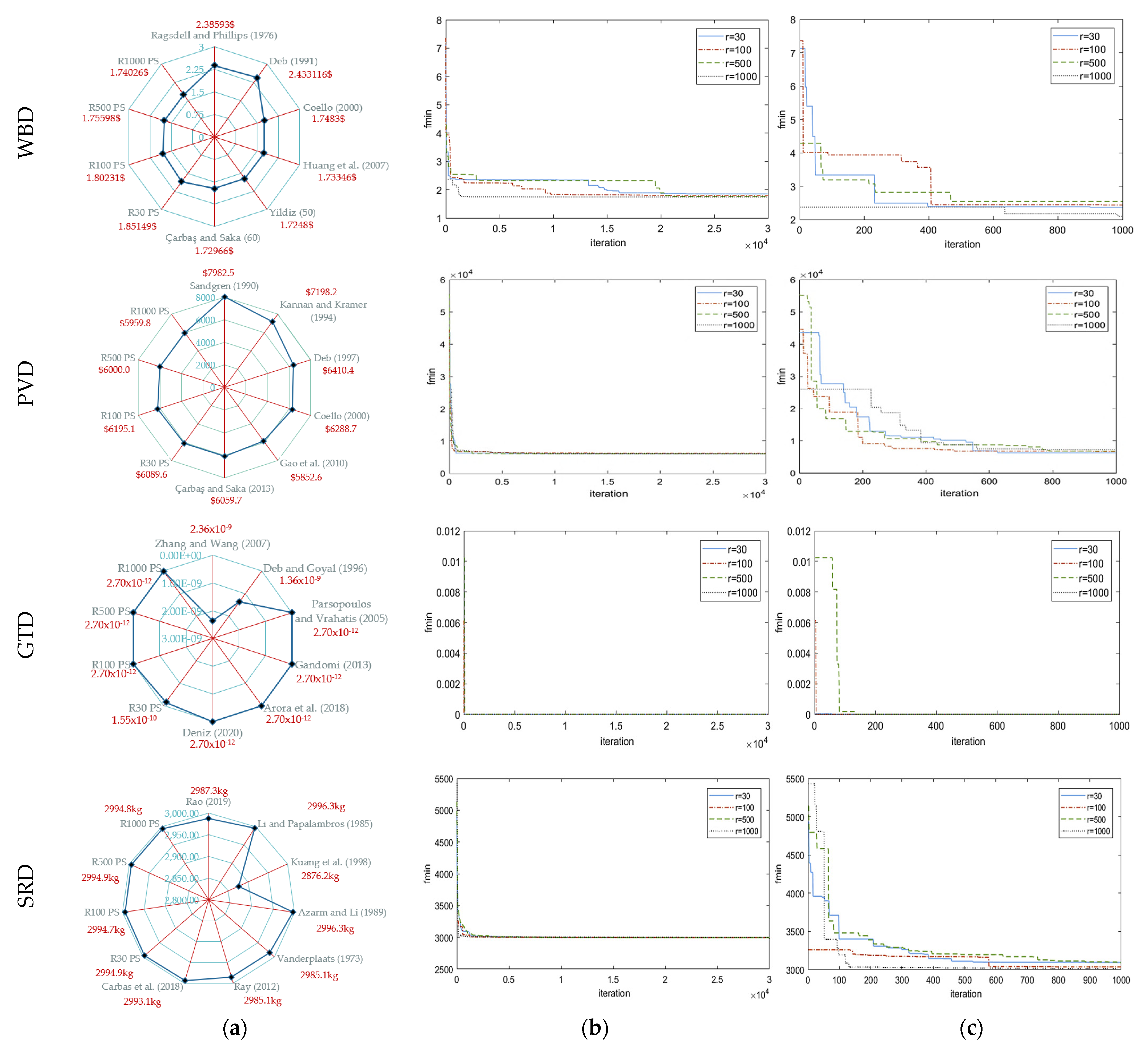
The minimum objective function value comparison between the previously reported studies in the literature which were conducted by utilizing different metaheuristic algorithms and the obtained results of design optimization problems are given for WBD, PVD, GTD, and SRD in Figure 6a [35,50,51,52,53,54,55,56,57,58,59,60,61,62,63,64,65,66,67,68,69,70]. In the same figure, general (b) and zoomed (c) view iteration history graphs of the best solution (fmin) for the best run among all runs are demonstrated. Detailed comparisons of results for design problems of WBD, PVD, GTD, and SRD with the studies in the literature are given for optimum solutions in

Table A1. Optimum values and comparison of the best solutions in literature for WBD.

Optimum Solutions		x1(h)(in.)	x2(l) (in.)	x3(t) (in.)	x4(b) (in.)	f(x) ($)
Literature	Ragsdell and Phillips [50]	0.24550	6.1960	8.2730	0.2455	2.38593
	Deb [51]	0.2489	6.173	8.1789	0.2533	2.433116
	Coello [52]	0.2088	3.4205	8.9975	0.21	1.7483
	Huang et al. [53]	0.203137	3.542998	9.033498	0.206179	1.73346
	Yildiz [54]	0.20573	3.47042	9.03649	0.205735	1.7248
	Çarbaş and Saka [55]	0.203907	3.499898	9.063898	0.205594	1.72966
Case PS	R30	0.206741	3.65285	8.54856	0.231265	1.85149
	R100	0.171535	4.42418	8.98313	0.208289	1.80231
	R500	0.198864	3.66442	8.94678	0.209895	1.75598
	R1000	0.19823	3.64539	9.02857	0.206407	1.74026
	WBD-5P	0.195872	3.70387	9.07235	0.205574	1.7455
	WBD-4P	0.188171	3.95948	8.91723	0.21133	1.78312

^PS Present study.

,

Table A2. Optimum values and comparison of the best solutions in literature for PVD.

Optimum Solutions		x1(Ts) (in.)	x2(Th) (in.)	x3(R) (in.)	x4(L) (in.)	f(x) ($)
Literature	Sandgren [35]	1.125	0.625	48.97	106.72	7982.5
	Kannan and Kramer [56]	1.25	0.625	50	120	7198.20
	Deb [57]	0.9375	0.50	48.329	112.679	6410.381
	Coello [52]	0.8125	0.4375	40.3239	200.0	6288.7445
	Gao et al. [58]	0.75	0.375	38.8441	221.612	5852.639
	Çarbaş and Saka [55]	0.8125	0.4375	42.09845	176.6366	6059.7143
Case PS	R30	0.876366	0.434563	45.3293	140.344	6089.66
	R100	0.915835	0.454142	47.2497	121.872	6195.1
	R500	0.833985	0.413952	43.1577	163.94	6000.09
	R1000	0.814181	0.403799	42.1533	176.032	5959.86
	PVD-5P	0.84119	0.430252	43.5749	159.245	6054.14
	PVD-4P	0.822121	0.409189	42.367	173.44	6005.19

^PS Present study.

,

Table A3. Optimum values and comparison of the best solutions in literature for GTD.

Optimum Solutions		x1(Ta) (piece)	x2(Tb) (piece)	x3(Td) (piece)	x4 (Tf) (piece)	Gear ratio	f(x) (unitless)
Literature	Zhang and Wang [59]	43	16	19	49	0.1442	2.36 × 10−9
	Deb and Goyal [60]	33	14	17	50	0.1442	1.362 × 10−9
	Parsopoulos and Vrahatis [61]	43	16	19	49	0.1442	2.701 × 10−12
	Gandomi [62]	43	16	19	49	0.1442	2.701 × 10−12
	Arora et al. [63]	43	16	19	49	0.1442	2.701 × 10−12
	Deniz [64]	43	16	19	49	0.1442	2.701 × 10−12
Case PS	R30	44	13	21	43	0.144292	1.54505 × 10−10
	R100	43	16	19	49	0.144281	2.70086 × 10−12
	R500	49	16	19	43	0.144281	2.70086 × 10−12
	R1000	49	16	19	43	0.144281	2.70086 × 10−12
	GTD-5P	49	16	19	43	0.144281	2.70086 × 10−12
	GTD-4P	49	16	19	43	0.144281	2.70086 × 10−12

^PS Present study.

and

Table A4. Optimum values and comparison of the best solutions in literature for SRD.

Optimum Solutions		x1 (cm)	x2 (cm)	x3 (piece)	x4 (cm)	x5 (cm)	x6 (cm)	x7 (cm)	f(x) (kg)
Literature	Li and Papalambros [65]	3.50	0.70	17.00	7.30	7.71	3.3500000	5.2900000	2996.30977
	Kuang et al. [66]	3.60	0.70	17.00	7.30	7.80	3.4000000	5.0000000	2876.22
	Azarm and Li [67]	3.50	0.70	17.00	7.30	7.71	3.3500000	5.2900000	2996.30978
	Vanderplaats [68]	3.50	0.70	17.00	7.30	7.30	3.3502145	5.2865176	2985.15188
	Ray [69]	3.50	0.70	17.00	7.30	7.30	3.3502145	5.2865176	2985.15188
	Carbas et al. [70]	3.50	0.70	17.00	7.17984	7.70889	3.35009	5.28668	2993.13917
Case PS	R30	3.5001	0.700016	17.0017	7.30052	7.71562	3.35025	5.28667	2994.93
	R100	3.50014	0.700021	17.0002	7.30117	7.71637	3.35053	5.28667	2994.79
	R500	3.50029	0.700019	17.0001	7.3009	7.71572	3.35053	5.28681	2994.90
	R1000	3.50025	0.700016	17.0004	7.30034	7.71652	3.35036	5.28673	2994.84
	SRD-5P	3.50184	0.700073	17.0008	7.3036	7.72133	3.35036	5.28679	2995.97
	SRD-4P	3.50006	0.700006	17.0034	7.30108	7.71868	3.3516	5.28677	2995.63

^PS Present study.

and for constraints in

Table A5. Constraint values of WBD, PVD, and SRD optimization problems.

		R30	R100	R500	R1000	5P	4P			R30	R100	R500	R1000	5P	4P
WBD	g1(x)	−8.821	−0.086	−7.948	−7.525	−65.745	−32.706	SRD	g1(x)	0.92592	0.92598	0.92595	0.92595	0.92536	0.92587
	g2(x)	−178.142	−14.670	−1.819	−45.079	−213.275	−7.722		g2(x)	0.80178	0.80190	0.80188	0.80187	0.80134	0.80165
	g3(x)	−0.025	−0.037	−0.011	−0.008	−0.010	−0.023		g3(x)	0.50085	0.50086	0.50081	0.50079	0.50141	0.50012
	g4(x)	−3.317	−3.338	−3.400	−3.414	−3.407	−3.368		g4(x)	0.09535	0.09539	0.09536	0.09539	0.09555	0.09545
	g5(x)	−0.082	−0.047	−0.074	−0.073	−0.071	−0.063		g5(x)	0.99994	0.99944	0.99944	0.99974	0.99975	0.99752
	g6(x)	−0.235	−0.235	−0.235	−0.236	−0.236	−0.235		g6(x)	0.99998	0.99998	0.99982	0.99991	0.99985	0.99987
	g7(x)	−2211.802	−202.416	−330.005	−55.908	−1.921	−446.574		g7(x)	0.29754	0.29751	0.29751	0.29751	0.29755	0.29756
PVD	g1(x)	−0.002	−0.002	−0.004	−0.001	−0.001	0.000		g8(x)	0.99999	0.99999	0.99994	0.99995	0.99958	0.99999
	g2(x)	−0.002	−0.002	−0.003	−0.002	−0.002	−0.015		g9(x)	0.41667	0.41667	0.41669	0.41669	0.41684	0.41667
	g3(x)	−89.466	−89.466	−636.323	−9.038	−412.835	−498.618		g10(x)	0.94861	0.94859	0.94862	0.94866	0.94824	0.94882
	g4(x)	−99.656	−99.656	−118.128	−76.060	−63.968	−80.755		g11(x)	0.99996	0.99987	0.99997	0.99986	0.99924	0.99958

of the Appendix A section.

It is seen that the optimal fmin value ($1.74026) acquired with the HSA algorithm when is R1000 case in this study is approximately 1% greater than the value ($1.7248) yielded with the hybrid Taguchi harmony search algorithm [54] according to comparison given in Figure 6a for WBD. The fmin value acquired as $5959.86 in the R1000 case for PVD is above the best fitness value with 2% ($5852.6394) presented according to the study by Gao et al. [58], which utilized the HSA with the bandwidth improvisation to the pitch adjustment rate. The reached optimum value of GTD in the R30 case which is 2.70086 × 10⁻¹² is the same as the best values presented in the literature [61,62,63,64]. The acquired optimum value (2994.79 kg) for SRD is higher than the best fitness value (2876.22 kg) presented in the literature study [66] with 4% obtained according to the Taguchi-aided optimization search method.

The comparison between obtained minimum objective function values of RCRW designs of the optimum cost (RCRW1) and the optimum weight (RCRW2) and the optimization study of retaining wall design in the literature are shown in Figure 7a [40]. The optimum search process at the run value which is the best solution (fmin) for R30, R100, R500, and R1000 is given as the general view and zoomed view of iteration history graphs in Figure 7b,c, respectively. Detailed results with the comparison of the optimum values in the literature for RCRW1 and RCRW2 designs are listed in

Table A6. Optimum values of RCRW design for the optimum cost (RCRW1).

Optimum Solutions		x1 (m)	x2 (m)	x3 (m)	x4 (m)	x5 (m)	x6 (m)	x7 (m)	x8 (cm2)	x9 (cm2)	x10 (cm2)	x11 (cm2)	x12 (cm2)	f(x) ($/kg)
Literature	Gandomi [40]	2.709	1	0.412	0.25	0.4	2.455	0.2	0.2	21.9911	11.7809	11.7809	4.7124	163.98
	Gandomi [40]	2.727	1.035	0.36	0.28	0.401	2.274	0.293	0.296	32.1699	13.3517	13.8544	8.6394	182.79
	Gandomi [40]	2.816	0.988	0.447	0.294	0.422	2.223	0.367	0.203	21.9911	15.2681	15.2681	12.7234	185.05
	Gandomi [40]	2.694	0.836	0.403	0.27	0.405	2.346	0.227	0.445	23.7504	12.7234	22.6195	26.1380	182.84
CasePS	R30	3.3439	1.1598	0.3526	0.2504	0.4	2.5435	0.2002	0.2	21.2999	14.3212	18.8016	7.1532	180.082
	R100	3.3431	1.1596	0.3917	0.25	0.4001	2.4623	0.2001	0.2002	18.8963	14.2586	18.9194	9.5172	179.842
	R500	3.3351	1.1593	0.4418	0.25	0.4001	3.0523	0.2004	0.2002	16.6776	14.3189	16.557	7.2319	179.449
	R1000	3.3394	1.1593	0.3916	0.2501	0.4	2.7275	0.2004	0.2003	18.691	14.392	18.7638	7.2583	179.693
	RCRW1−5P	3.36761	1.15955	0.391877	0.250366	0.400094	2.84595	0.200248	0.201545	18.7689	14.4128	18.7273	10.0995	181.035
	RCRW1−4P	3.34757	1.15992	0.394711	0.250081	0.400157	2.37294	0.202173	0.201494	18.7718	14.1765	18.7523	9.34978	180.301

^PS Present study.

and

Table A7. Optimum values of RCRW design for the optimum weight (RCRW2).

Optimum Solutions		x1 (m)	x2 (m)	x3 (m)	x4 (m)	x5 (m)	x6 (m)	x7 (m)	x8 (cm2)	x9 (cm2)	x10 (cm2)	x11 (cm2)	x12 (cm2)	f(x) ($/kg)
Literature	Gandomi [40]	2.709	1	0.412	0.25	0.4	2.455	0.2	0.2	21.9911	11.7809	11.7809	4.7124	5668.5
	Gandomi [40]	2.727	1.035	0.36	0.28	0.401	2.274	0.293	0.296	32.1699	13.3517	13.8544	8.6394	6034.4
	Gandomi [40]	2.816	0.988	0.447	0.294	0.422	2.223	0.367	0.203	21.9911	15.2681	15.2681	12.7234	6095.9
	Gandomi [40]	2.694	0.836	0.403	0.27	0.405	2.346	0.227	0.445	23.7504	12.7234	22.6195	26.1380	6094.4
CasePS	R30	3.342	1.1599	0.2505	0.2504	0.4	3.1292	0.2001	0.2001	35.1479	14.1715	21.5672	7.0299	5886.67
	R100	3.3426	1.16	0.2501	0.2501	0.4	3.0709	0.2001	0.2002	35.1127	15.0607	21.2321	7.0677	5883.61
	R500	3.343	1.1581	0.25	0.25	0.4001	3.0355	0.2001	0.2002	35.247	14.4184	21.3267	7.3429	5883.64
	R1000	3.3434	1.1594	0.2501	0.25	0.4	3.1304	0.2001	0.2001	35.2741	14.1095	21.2558	9.3741	5884.09
	RCRW1−5P	2.709	1	0.412	0.25	0.4	2.455	0.2	0.2	21.9911	11.7809	11.7809	4.7124	5668.5
	RCRW1−4P	2.727	1.035	0.36	0.28	0.401	2.274	0.293	0.296	32.1699	13.3517	13.8544	8.6394	6034.4

^PS Present study.

of the Appendix A section, respectively.

According to the comparison of optimum designs with the literature studies given in Figure 7a, it is obvious that RCRW1 and RCRW2 optimum objective function values ($179.4495/m and 5883.61 kg/m) are greater than the best values ($163.98/m and 5668.5 kg/m) presented by Gandomi et al. [40] as 9% and 4%, respectively. In this study, it has been determined that the optimum solutions yielded by the HSA for two different objective functions of a real size engineering design optimization problem are close to the literature values which were reached by using different algorithms in general for comparison. Although it is presented as the best solution acquired with the biogeography-based optimization (BBO) algorithm considering the optimization problem, it is not specified whether the optimum solution of the 26 constraints utilized in the study is provided. Since it is important to obtain the best solution that provides all constraints of the optimization problem, the values of the constraints accomplished for this study, in which the mathematical model of the optimization problem is compared, are given in

Table A8. Constraint values of RCRW designs for optimum cost and optimum weight.

	Optimum Cost (RCRW1)						Optimum Weight (RCRW2)
	R30	R100	R500	R1000	5P	4P	R30	R100	R500	R1000
g1(x)	−0.0462	−0.043	−0.037	−0.0421	−0.0497	−0.0441	−0.0536	−0.0537	−0.0543	−0.0541
g2(x)	−0.638	−0.6334	−0.6224	−0.6305	−0.6613	−0.6376	−0.6468	−0.6472	−0.648	−0.6484
g3(x)	−2.5539	−2.569	−2.5824	−2.5638	−2.6425	−2.5813	−2.5106	−2.5112	−2.5092	−2.5137
g4(x)	−0.1129	−0.1141	−0.0221	−0.0199	−1.8384	−0.3677	−0.0072	−0.0142	−0.0149	−0.0925
g5(x)	−0.0001	−0.0004	0.0000	−0.0002	−0.0009	−0.0085	−0.0633	−0.0615	−0.061	−0.0615
g6(x)	−0.4023	−0.4058	−0.4103	−0.4057	−0.4115	−0.4066	−0.3937	−0.4242	−0.3951	−0.3944
g7(x)	−0.0326	−0.0701	−0.0052	−0.0728	−0.0531	−0.07	−0.062	−0.0482	−0.0464	−0.0472
g8(x)	−0.9964	−0.9973	−0.9964	−0.9964	−0.9974	−0.9973	−0.9964	−0.9964	−0.9964	−0.9973
g9(x)	−0.3955	−0.4637	−0.5333	−0.4635	−0.464	−0.4684	−0.1169	−0.1154	−0.115	−0.1154
g10(x)	−0.4032	−0.4065	−0.4107	−0.4064	−0.4096	−0.407	−0.3956	−0.3955	−0.3964	−0.3959
g11(x)	−0.065	−0.0845	−0.1132	−0.0858	−0.0767	−0.0847	−0.0179	−0.0175	−0.0167	−0.017
g12(x)	−0.9936	−0.9935	−0.9936	−0.9935	−0.9934	−0.9936	−0.9935	−0.9935	−0.9935	−0.9935
g13(x)	−0.4189	−0.2727	−0.0625	−0.2729	−0.2724	−0.2671	−0.7519	−0.7523	−0.7524	−0.7523
g14(x)	−0.0097	−0.0095	−0.0095	−0.0097	−0.0095	−0.0093	−0.0097	−0.0618	−0.0095	−0.0097
g15(x)	−0.2573	−0.2571	−0.151	−0.2573	−0.2571	−0.257	−0.3504	−0.3408	−0.3406	−0.3408
g16(x)	−0.0087	−0.2569	−0.0077	−0.0077	−0.3028	−0.2492	−0.0092	−0.0092	−0.0092	−0.2569
g17(x)	−0.6471	−0.7181	−0.7813	−0.718	−0.7182	−0.7202	−0.1734	−0.1721	−0.1718	−0.1721
g18(x)	−0.7929	−0.793	−0.793	−0.7929	−0.793	−0.793	−0.7929	−0.7814	−0.793	−0.7929
g19(x)	−0.7239	−0.724	−0.7585	−0.7239	−0.724	−0.724	−0.6844	−0.689	−0.689	−0.689
g20(x)	−0.7931	−0.7241	−0.7934	−0.7934	−0.7059	−0.7269	−0.793	−0.793	−0.793	−0.7241
g21(x)	−0.5477	−0.536	−0.5199	−0.5356	−0.5393	−0.5356	−0.578	−0.5781	−0.5788	−0.5784
g22(x)	−0.1795	−0.2036	−0.0247	−0.1232	−0.0954	−0.2308	−0.0038	−0.0214	−0.0321	−0.0039
g23(x)	−0.2382	−0.3654	−0.3654	−0.3652	−0.3654	−0.3655	−0.3652	−0.3652	−0.3654	−0.3652
g24(x)	−0.6364	−0.6365	−0.6365	−0.6364	−0.6365	−0.6365	−0.6364	−0.4909	−0.6365	−0.6364
g25(x)	−0.6364	−0.6365	−0.6365	−0.6364	−0.6365	−0.6365	−0.4182	−0.5636	−0.5638	−0.5636
g26(x)	−0.1113	−0.3654	−0.1115	−0.1113	−0.1115	−0.3655	−0.1113	−0.1113	−0.1115	−0.3652

of the Appendix A section.

Conducted analyses have been shown that the appropriate numbers of iteration and the independent run of entire iterations, which formed the extent of the acquiring optimum process, are significant to reaching the best fitness value instead of many or fewer numbers of them. The reaching process of the maximum iteration number defined as the run is accepted 30 times in the literature of optimization studies and the most minimum fitness value satisfying the design constraints is presented as the optimum result. The minimum fitness values have been yielded by operating different design problems with different runs when the number of the runs is greater than 30 according to the results given in the tables. It observed that while the more minimum fitness values generally are obtained with the increasing runs in some engineering design problems, the minimum result may not be found with larger runs too in some of them. This brings to the fore the necessity that the number of executions of the optimization algorithm may have an optimum value.

3.2. Taguchi Analyses

The best combination, which provided the best fitness value for the welded beam design (WBD), the pressure vessel design (PVD), the gear tear design (GTD), the speed reducer design (SRD), the reinforced concrete cantilever retaining wall design (RCRW1) optimization problems have been investigated in terms of design parameters effective on the searching optimum solutions via the Taguchi method integrated hybrid harmony search algorithm (TIHHSA) as visualized in Figure 5.

3.2.1. Part I: Investigation of Five Optimum Design Parameter Values with Effect on the Fitness Value

For the abovementioned aim, by considering different values of design parameters, the harmony memory size (HMS), the harmony memory consideration rate (HMCR), the pitch adjustment rate (PAR), maximum iteration number (MAXITER), and the independent run number of the whole iterations (RUN), 16 designs given in Table 4 formed according to L16 orthogonal array have been performed. By utilizing obtained the minimum objective function values, f(x), for each design optimization problem, the Signal/Noise ratios (S/N), defined in Equation (4) with the aim of the case of smaller is better, have been calculated and listed with the response values of different engineering design optimization problems in

Table 7. Response values (f(x)) and S/N ratios of response values.

Design No	f(x)					S/N
	WBD ($)	PVD ($)	GTD (Unitless)	SRD (kg)	RCRW1 ($/kg)	WBD	PVD	GTD	SRD	RCRW1
1	2.1880	6595.36	9.94 × 10−11	3002.24	196.841	−6.8010	−76.38	200.052	−69.5489	−45.882
2	1.8766	6315.66	2.70 × 10−12	2996.59	183.264	−5.4672	−76.01	231.37	−69.5325	−45.262
3	1.8656	6040.75	2.70 × 10−12	2996.09	181.325	−5.4165	−75.62	231.37	−69.5311	−45.169
4	1.8073	5985.52	2.70 × 10−12	2996.03	180.652	−5.1405	−75.54	231.37	−69.5309	−45.137
5	1.8383	6039.20	2.70 × 10−12	2995.6	183.881	−5.2881	−75.62	231.37	−69.5297	−45.291
6	1.8528	6014.33	2.70 × 10−12	2995.81	181.395	−5.3564	−75.58	231.37	−69.5303	−45.173
7	2.1053	6116.35	2.31 × 10−11	3002.82	189.297	−6.4661	−75.73	212.736	−69.5506	−45.543
8	2.5046	6389.99	2.70 × 10−12	3001.70	187.417	−7.9747	−76.11	231.37	−69.5474	−45.456
9	2.1041	6257.68	2.70 × 10−12	2996.93	185.566	−6.4615	−75.93	231.37	−69.5335	−45.370
10	2.0103	6385.19	9.94 × 10−11	2998.29	186.013	−6.0654	−76.10	200.052	−69.5375	−45.391
11	1.7921	6105.73	2.70 × 10−12	2997.21	183.491	−5.0673	−75.71	231.37	−69.5343	−45.272
12	2.0951	6286.05	2.70 × 10−12	3000.60	188.117	−6.4240	−75.97	231.37	−69.5442	−45.489
13	1.9126	6136.63	2.70 × 10−12	2998.17	190.651	−5.6324	−75.76	231.37	−69.5371	−45.605
14	2.0021	6169.29	2.70 × 10−12	3002.63	195.777	−6.0298	−75.80	231.37	−69.550	−45.835
15	1.9833	6186.53	2.70 × 10−12	2998.66	183.548	−5.9477	−75.83	231.37	−69.5386	−45.275
16	2.1366	6147.29	2.70 × 10−12	2997.24	183.776	−6.5943	−75.77	231.37	−69.5344	−45.286
η	2.0047	6198.22	1.61 × 10−11	2998.50	186.313	−6.0083	−75.84	226.29	−69.5382	−45.402

.

The rank (R) which indicates the order of design parameters effect from largest to smallest have been accomplished by using η_ij values for each design optimization problem. The sum of squares (SS), variance (ν), and rank (R) values acquired from ANOVA analyses are demonstrated in

Table 8. Results of variance analyses of WBD, PVD, GTD, SRD, and RCRW1 optimization problems.

Optimization Problem	Evaluation Criteria	Design Parameter
		HMS	HMCR	PAR	MAXITER	RUN
WBD	SS	0.6492	1.7416	1.2039	1.1445	4.0607
	ν	0.216309	0.580439	0.401491	0.381525	1.35359
	R	5	2	3	4	1
PVD	SS	0.0754	0.0865	0.0188	0.1542	0.4473
	ν	0.02515	0.028833	0.006269	0.051393	0.149109
	R	4	3	5	2	1
GTD	SS	164.432	164.432	456.416	456.416	654.917
	ν	54.8032	54.8032	152.065	152.065	218.268
	R	4	5	2	3	1
SRD	SS	4.44 × 10−5	9.58 × 10−6	4.53 × 10−5	6.15 × 10−4	1.36 × 10−4
	ν	1.48 × 10−5	3.21 × 10−6	1.51 × 10−5	2.05 × 10−4	4.55 × 10−5
	R	4	5	3	1	2
RCRW1	SS	0.052	0.1184	0.0349	0.4879	0.0535
	ν	0.0173	0.0395	0.0116	0.1626	0.0179
	R	4	2	5	1	3

. The Taguchi method which is a fractional factorial design is a saturated model [71,72]. It means that all degrees of freedom are used in the estimation. For this reason, p values are not given in Table 8 as no residual error occurs in the Taguchi design with L₁₆(4)⁵. While the RUN is the most effective parameter being that the biggest variance value having for WBD, PVD, and GTD designs, the MAXITER is the most important parameter for SRD and RCRW1 in reaching minimum objective function. Although the possibility of obtaining the more minimum or the most minimum fitness value is triggered by extending the optimization process with more iteration such as SRD and RCRW1 designs, it occurs the outcome that unavailability of no more optimum values with continuing analyses and needed for a new independent run process such as WBD, PVD, and GTD problems.

It is observed from the variance results that the PAR and the HMS have an average or minimal effect with rank values of 3 or 5 and 3, 4 or 5. In improvising a new solution of the HSA, if the assigned random number is smaller than HMCR, the PAR is compared to a new random number. In satisfying this condition, the solution is improved, and its new fitness value is determined. As including the PAR in this process depends on the possibility of an assigned random number, it is commented that the PAR may not be a much effective parameter to find the minimum except for the GTD problem. The PAR is the second effective design parameter on the best fitness value for GTD which is an unconstrained design problem. The HMS design parameter may not be the most critical one since the solutions of HM become the same each other with increasing iteration for each different run to reach the fmin.

In addition, the prediction of the response value (η_prediction), and the optimum parameter combination have been determined separately for each design problem (

Table 9. Verification analyses data and results with optimum values of design parameters.

Optimization Problem	Optimum Parameter Combination	fmin (ηprediction)
WBD	HMS1-HMCR3-PAR2-MAXITER4-RUN4	$1.63817
PVD	HMS2-HMCR3-PAR4-MAXITER4-RUN4	$5813.73
GTD	HMS4-HMCR4-PAR2-MAXITER2-RUN3	2.60398 × 10−12
SRD	HMS1-HMCR1-PAR2-MAXITER3-RUN3	2994.16 kg
RCRW1	HMS1-HMCR3-PAR2-MAXITER4-RUN3	$177.724/m

). The real response values (η_real) which are specified by considering the optimum parameter combination have been obtained with verification analyses (

Table 10. Statistical results from verification analyses of engineering design optimization problems.

Case	Run						Iteration
	BRN	Best (ηreal)	Mean	Worst	StD	Median	BIN	Best (ηreal)	Mean	Worst	StD	Median
WBD	202/1000(20%)	1.7455	2.8743	5.10816	0.54932	2.8190	2598/8000 (32%)	1.7455	1.82	9.44763	0.418665	1.7455
PVD	897/1000(89%)	6054.14	7000.4	8272.08	427.637	7032.49	7828/8000 (98%)	6054.14	7153.31	42,950.5	3947.25	6180.14
GTD	2/500 (0.4%)	2.70086 × 10−12	5.4247 × 10−8	1.38114 × 10−6	1.34484 × 10−7	1.31252 × 10−8	312/4000 (8%)	2.70086 × 10−12	2.99998 × 10−5	5.5068 × 10−3	3.7964 × 10−3	2.70086 × 10−12
SRD	399/500 (80%)	2995.97	3004.43	3022.88	4.62559	3003.84	5746/6000 (96%)	2995.97	3062.32	5322.68	296.145	2996.6
RCRW1	425/500 (85%)	181.035	191.431	206.659	5.36727	191.363	7740/8000 (97%)	181.035	199.648	386.834	38.1441	189.368

).

Since the optimum values of MAXITER and RUN have been accomplished as their maximum values (MAXITER = 6000 and 8000 and RUN = 500 and 1000) for different optimization design problems except for GTD, it is concluded that finding more fitness values are needed more research process for constrained optimization design problems. Generally, it is detected from the yielded results that the optimum values of algorithm parameters of HSA (HMS, HMCR, PAR) have been altered according to the characteristics of the design problem. In cases with smaller HMS values (20, 30) for WBD, PVD, and RCRW1, the large HMCR value (0.90) has increased the probability that the new solutions improvised in the algorithm is selected from the HM, while the new solution has been randomly selected from the design space with the possibility of small HMCR value (0.80) for SRD. The GTD unconstrainted design problem whose optimum values are obtained for HMS = 50 and HMCR = 0.95 shows that the optimum search has been sufficient with fewer iterations and runs due to the different characteristics of the design optimization problem and its small size.

3.2.2. Part II: Investigation of Four Optimum Design Parameter Values with Effect on the Fitness Value

It is apparent from analyses that the most effective algorithm parameter for reaching the best fitness value is mostly the RUN with S/N ratios and a change percentage of parameter effect for the 5P case. Furthermore, the minimum objective function value is estimated via the TIHHSA, when the optimum RUN value equals 1000 for WBD and PVD and 500 for GTD, SRD, and RCRW1 problems. For this reason, the S/N ratios, variance, and optimum Taguchi parameter values have been repeated by analyses which are taken as fix values whose optimum RUN value for four parameters (the 4P case) to reasonably observe the parameter effect of the other design parameters. According to DM given in the first section of

Table 11. Response values (f(x)) and S/N ratios of response values.

	DM						f(x)					S/N
Design No	HMS	HMCR	PAR	MAXITER	RUN
					WBD PVD	GTD SRDR CRW1	WBD ($)	PVD ($)	GTD (Unitless)	SRD (kg)	RCRW1 ($/kg)	WBD	PVD	GTD	SRD	RCRW1
1	20	0.80	0.10	2000	1000	500	1.8162	6105.21	2.70 × 10−12	3000.31	190.785	−5.1831	−75.71	231.37	−69.54	−45.611
2	20	0.85	0.20	4000	1000	500	1.7882	6029.48	2.70 × 10−12	2996.04	183.739	−5.0485	−75.61	231.37	−69.53	−45.284
3	20	0.90	0.30	6000	1000	500	1.8059	5978.28	2.70 × 10−12	2996.04	182.141	−5.1340	−75.53	231.37	−69.53	−45.208
4	20	0.95	0.40	8000	1000	500	1.8331	6033.37	2.70 × 10−12	2996.22	180.155	−5.2637	−75.61	231.37	−69.53	−45.113
5	30	0.80	0.20	6000	1000	500	1.7931	6055.08	2.70 × 10−12	2996.34	182.660	−5.0721	−75.64	231.37	−69.53	−45.233
6	30	0.85	0.10	8000	1000	500	1.7869	5999.42	2.70 × 10−12	2996.01	181.975	−5.0420	−75.56	231.37	−69.53	−45.200
7	30	0.90	0.40	2000	1000	500	1.8419	6127.22	2.70 × 10−12	3000.97	189.144	−5.3055	−75.75	231.37	−69.55	−45.536
8	30	0.95	0.30	4000	1000	500	1.7892	6052.60	2.70 × 10−12	2997.24	183.061	−5.0532	−75.64	231.37	−69.53	−45.252
9	40	0.80	0.30	8000	1000	500	1.9165	6003.01	2.70 × 10−12	2996.23	184.049	−5.6501	−75.57	231.37	−69.53	−45.299
10	40	0.85	0.40	6000	1000	500	1.8280	6044.31	2.70 × 10−12	2996.86	182.456	−5.2397	−75.63	231.37	−69.53	−45.223
11	40	0.90	0.10	4000	1000	500	1.8945	6098.92	2.70 × 10−12	2997.09	182.774	−5.5498	−75.71	231.37	−69.53	−45.238
12	40	0.95	0.20	2000	1000	500	2.1363	6034.29	2.70 × 10−12	3002.13	189.270	−6.5932	−75.61	231.37	−69.55	−45.542
13	50	0.80	0.40	4000	1000	500	1.9349	6087.48	2.70 × 10−12	2997.00	190.329	−5.7333	−75.69	231.37	−69.53	−45.590
14	50	0.85	0.30	2000	1000	500	1.9848	6213.94	2.70 × 10−12	3001.98	199.838	−5.9544	−75.87	231.37	−69.55	−46.014
15	50	0.90	0.20	8000	1000	500	1.8826	6073.32	2.70 × 10−12	2995.93	180.585	−5.4950	−75.67	231.37	−69.53	−45.134
16	50	0.95	0.10	6000	1000	500	2.0482	6091.36	2.70 × 10−12	2997.44	182.249	−6.2276	−75.69	231.37	−69.54	−45.213
	η						1.8800	6064.21	2.70 × 10−12	2997.74	185.326	−5.4716	−75.66	231.37	−69.54	−45.356

, optimization analyzes have been performed and then response values given in the second section of Table 11 have been obtained.

In contrast to the Taguchi design with L₁₆(4)⁵, obtained p values with SS and R values which are due to the reduction of the number of parameters for the Taguchi design with L₁₆(4)⁴ are given in

Table 12. Results of variance analyses of WBD, PVD, GTD, SRD, and RCRW1 optimization problems.

Optimization Problem	Evaluation Criteria	Design Parameter
		HMS	HMCR	PAR	MAXITER
WBD	SS	1.803926	0.53773	0.061213	0.45212
	ν	0.60131	0.17924	0.020407	0.150711
	p	0.100039	0.353229	0.901733	0.405384
	R	1	2	4	3
PVD	SS	0.031716	0.001684	0.003575	0.040544
	ν	0.0105718	0.000560958	0.00119166	0.0135146
	p	0.405366	0.971217	0.921773	0.332366
	R	2	4	3	1
SRD	SS	1.98 × 10−5	1.33 × 10−6	1.20 × 10−6	5.93 × 10−6
	ν	6.57677 × 10−6	4.40671 × 10−6	4.02287 × 10−7	1.97717 × 10−4
	p	0.046127	0.077733	0.658534	0.000333
	R	3	2	4	1
RCRW1	SS	0.094191	0.092708	0.050628	0.598937
	ν	0.0314006	0.0309005	0.0168764	0.199651
	p	0.141871	0.144468	0.272054	0.012293
	R	2	3	4	1

. The variance values (Table 12) have been specified by utilizing the S/N ratios (the third section of Table 11) have been calculated with the aim of smaller is the best. MAXITER is the most effective algorithm parameter according to variance and rank values for PVD, SRD, and RCRW1 design optimization problems. While the MAXITER has the first rank value for SRD and RCRW1 problems whose sizes are higher than the others due to the number of design constraints and design variables, it hasn’t been a critical factor for the WBD problem. The HMS and HMCR design parameters are the first and second effective factors, respectively. It is noticed that the HMCR and PAR design parameters, which are included in the process of reaching the best solution according to the random number assigned in the algorithm, generally have lower variance. Conducting the statistical analysis with four design parameters instead of five has not shown reasonable and changing results for the GTD problem which is unconstrained and has a relatively small problem size.

In

Table 13. Verification analyses data and results with optimum values of design parameters.

Optimization Problem	Optimum Parameter Combination	fmin (ηprediction)
WBD	HMS2-HMCR2-PAR4-MAXITER2	$1.7291
PVD	HMS1-HMCR4-PAR2-MAXITER4	$5973.13
GTD	HMS1-HMCR1-PAR1-MAXITER1	2.70086 × 10−12
SRD	HMS1-HMCR1-PAR2-MAXITER4	2995.11 kg
RCRW1	HMS1-HMCR3-PAR2-MAXITER4	$177.842/m

, the prediction of the response value (η_prediction), and the optimum parameter combination have been demonstrated for each design problem. In verification analyses, the minimum objective function values (η_real) with the statistical evaluations have been obtained for estimated optimum values of design parameters (

Table 14. Statistical results from verification analyses of engineering design optimization problems.

Case	Run						Iteration
	BRN (%)	Best (ηreal)	Mean	Worst	StD	Median	BIN (%)	Best (ηreal)	Mean	Worst	StD	Median
WBD	373/1000(37%)	1.78312	1.88853	6.22216	0.320969	1.82613	3561/4000 (89%)	1.78312	2.82897	4.61973	0.492371	2.74472
PVD	881/1000 (88%)	6005.19	7125.64	8728.03	503.107	7169.81	7870/8000 (%98)	6005.19	7442.32	67288.7	3342.35	6395.62
GTD	89/500 (%18)	2.70086 × 10−12	5.4247 × 10−8	1.38114 × 10−6	1.34484 × 10−7	1.31252 × 10−8	1250/2000 (63%)	2.70086 × 10−12	2.99998 × 10−5	5.5068 × 10−3	3.7964 × 10−3	2.70086 × 10−12
SRD	195/500 (40%)	2995.63	3002.75	3275.14	13.0823	3001.31	7187/8000 (90%)	2995.63	3037.28	5194.7	234.639	2998.37
RCRW1	460/500 (92%)	180.301	190.495	206.994	5.28013	190.4	7841/8000 (98%)	180.301	204.729	385.939	48.688	188.459

). While the optimum value of MAXITER has been found as its maximum level as 4 (8000) for PVD, SRD, and RCRW1, its optimum level is 2 (4000) and 1 (2000) for WBD and GTD, respectively. It is observed that the optimum level of HMS is equal to 1 (20) for all optimization design problems except for WBD to reach the minimum objective function. Consequently, it is concluded that the optimum values of HSA parameters act upon properties of the considered design optimization problem although the convergence of the minimum fitness value has increased with many iterations.

4. Discussion

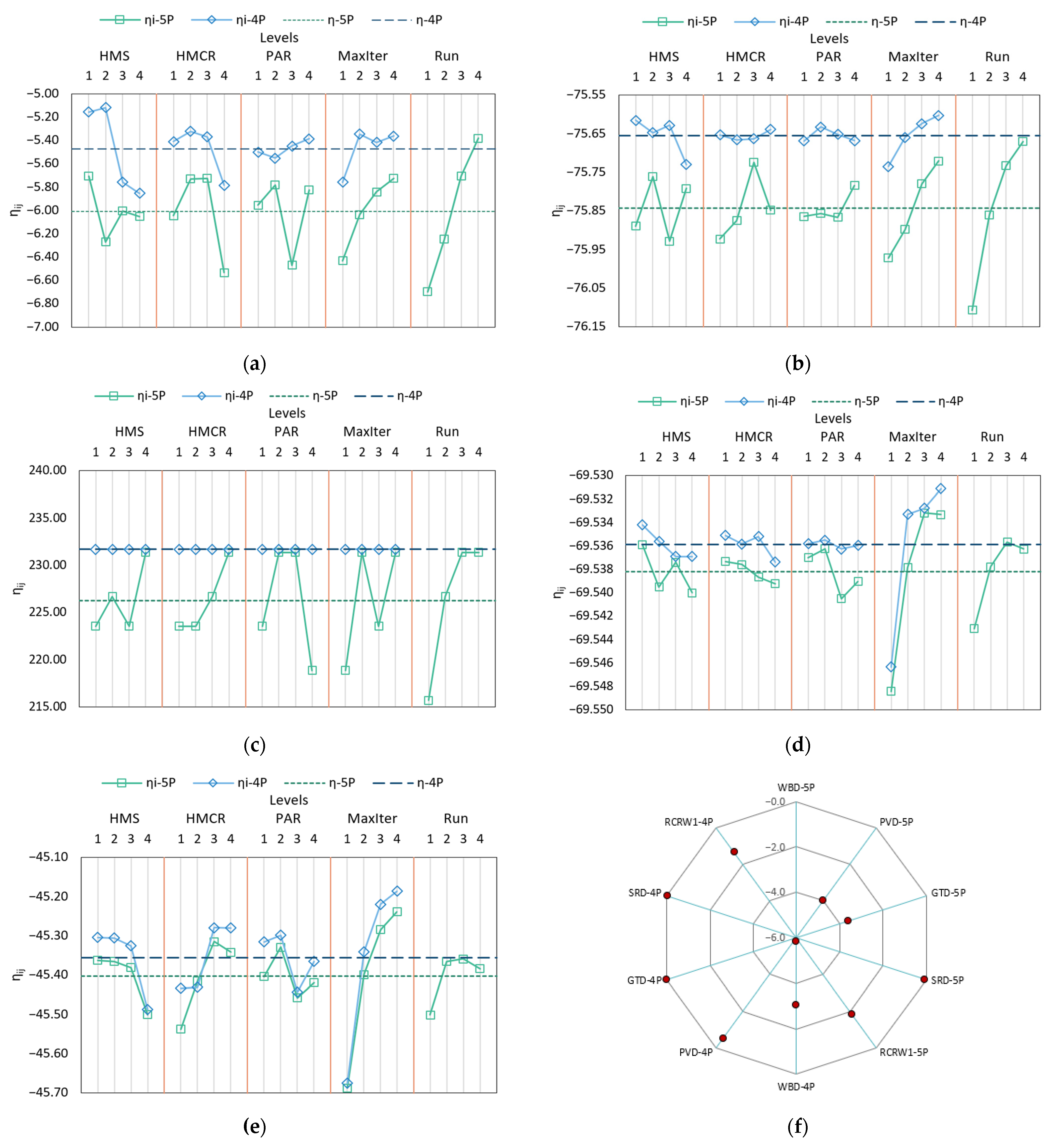
In this section, yielded results from optimization and statistical analyses by utilizing proposed TIHHSA with different design parameters have been evaluated in terms of different design optimization problems. In addition, the examination of the change of design parameters for different design problems in terms of 5P and 4P cases has been made according to the comparison graphics given in Figure 8 and Figure 9. By utilizing S/N ratios, the η_ij values have been determined and the variation between response value and design parameter levels are demonstrated for each design optimization problem according to five design parameters (the 5Pcase) and four design parameters (the 4P case) as shown in Figure 8a–e.

The S/N ratios which are control parameters in the Taguchi design supply information about the variation of the design parameters in different levels. In variation evaluations of η_ij values based on S/N ratios, three features have been observed. The first feature is belonging to the WBD problem with four design variables and seven design constraints and the PVD problem with four design variables and three design constraints and it is detected that there is an important change between S/N ratios of 5P and 4P. It is assumed that the contributions of other design parameters (HMS, HMCR, PAR, and MAXITER) are perceived more clearly, since the RUN parameter, which has the most variation in the 5P case, is taken as constant for its optimum value in the 4P case. The second feature, which has not emerged any change from 5P to 4P, is observed for the GTD problem with four design variables and no design constraints. It has been interpreted as no change because there are no design constraints, and it is a relatively small-size design optimization problem. The third feature has been determined for large-size design optimization problems which are SRD with seven design variables and eleven design constraints and RCRW1 with twelve design variables and twenty-six design constraints. As it has been apparent in the figures, since the RUN design parameter is not significantly effective in the 5P case, there is no significant change in other parameters in the 4P case.

The parameter percentage (PE, %) values which are based on the sum of squares values acquired from variance analyses are demonstrated for 4P and 5P cases of all design optimizations problems in Figure 9. In the 4P case where the RUN design parameter is taken as constant for depending on optimum values of the current design optimization problem, an increase has been monitored in the PE values yielded for the HMS, HMCR, PAR, and MAXITER design parameters compared to the 5P case. The PE values of the RUN design parameter in the 5P case have been obtained 46%, 57%, 35%, 16%, and 7% for WBD, PVD, GTD, SRD, and RCRW1 problems, respectively. When the PE values 4P and 5P cases have been compared in terms of changes in MAXITER values, it has been seen that the PE values have increased from 13% to 16% for WBD, from 20% to 52% for PVD, from 24% to 25% for GTD, from 72% to 95% for SRD and from 65% to 72% for RCRW1 problem. The HMS, HMCR, PAR, MAXITER and RUN design parameters have been the most effective factor for cases of WBD-4P (63%), GTD-4P (25%), GTD-4P (25%), SRD-4P (95%), and PVD-5P (57%), respectively.

When the optimum design parameter combinations estimated for the 4P and 5P cases of different design optimization problems (Figure 10) are compared, it is detected that a generalization cannot be made because it changes depending on the nature of the design optimization problem. This result has recognized that taking into account the different number of design variables, the process of reaching the best solution providing many design constraints has occurred differently for especially HSA design parameters. While the η_real values for 5P case have been accomplished as $1.7455, $6054.14, 2.70 × 10⁻¹², 2995.97 kg and 181.035 ($/m), they have been found for 4P case as $1.78312, $6005.14, 2.70 × 10⁻¹², 2995.63 kg, and 180.301($/m) for WBD, PVD, GTD, SRD, and RCRW1 problems, respectively. Except for the WBD problem with 2% of change, it has not been found more minimum objective function values. When the relative error (ε, %) values, which are calculated by using η_real and η_prediciton, for all design optimization problems and the cases have been examined, the maximum ε value has been marked as 6% (Figure 8f).

A comparison of the best fitness values presented in this study with those reported in the literature [73], which was shared the best fitness values of HSA and their variant, has been conducted for the WBD design optimization problem. When the mentioned study has been examined in terms of the best fitness value and the optimum values of the HS algorithm, it is seen that fmin value ($1.72489123) is obtained for HMS = 8, HMCR = 0.80, PAR = 0.30, and MaxIter = 200,000. In this study, the fmin value has been estimated as $1.7291 and has been found as $1.7455 with verification analyses at HMS = 20, HMCR = 0.95, PAR = 0.20, MAXITER = 8000, and RUN = 1000. These results show that it is possible to convergence to the best fitness value with fewer iterations in the optimization process. Besides, it is concluded that the fmin value ($1.7455) is reasonable according to compared with the optimum values acquired for other heuristic optimization methods given in Table A1 of the Appendix A section. Being almost the close fmin values eachother show that the Taguchi method is an alternative and effective in estimating the optimum algorithm parameter values of HSA.

The optimum values of MAXITER and RUN have been found as their maximum values (MAXITER = 6000 and 8000 and RUN = 500 and 1000) for different optimization design problems, except for GTD. While the f(x) minimum values of WBD and PVD for HMS = 20, HMCR = 0.90, PAR = 0.35, MAXITER= 30,000 and RUN = 1000 have been obtained as $1.74026 and $5959.86, the same values of GTD and SRD for HMS = 20, HMCR = 0.90, PAR = 0.35, MAXITER = 30,000 and RUN = 100 have been found as 2.70086 × 10⁻¹² and 2994.79 kg (Table 5). While fmin (η_real) of WBD $1.7455 which is quite close to $1.74026 has been found for HMS = 20, HMCR = 0.90, PAR = 0.20, MAXITER = 8000 and RUN = 1000, fmin (η_real) of PVD $6054.14 which is quite close to $5959.86 too has been found for HMS = 30, HMCR = 0.90, PAR = 0.40, MAXITER = 8000 and RUN = 1000.

5. Conclusions

In this study, optimum values of harmony search algorithm (HSA) design parameters, which are the harmony memory size (HMS), the harmony memory consideration rate (HMCR), the pitch adjustment rate (PAR), maximum iteration number (MAXITER), and the independent run number of whole iterations (RUN), have been investigated for complex benchmark engineering design problems (the welded beam (WBD), the pressure vessel (PVD), the gear train (GTD), and the speed reducer (SRD)) and complicated real-size reinforcement cantilever retaining wall (RCRW) design problem. To examine the optimum values of algorithm design parameters, the Taguchi method integrated hybrid harmony search algorithm (TIHHSA) has been presented as a new hybrid method based on the Taguchi Method which is a statistical-based experiment procedure utilized in boosting algorithmic quality. In addition, the effect of algorithm design parameters on the best fitness value and characteristics of the optimization problem has been studied. The results yielded according to the optimum algorithm design parameters and the best fitness values, whose values do not change with repetitive statistical, and optimization analyzes for different engineering design optimization problems, are as follows;

Accomplished results from the Taguchi analyses show that converging to the best fitness value is possible with fewer iteration numbers in a shorter time;

• The obtained estimations have a reasonable relative error in determining optimum values of algorithm design parameters without performing many trials;
• It has been seen that the optimum values of the algorithm design parameters vary depending on the nature of the design optimization problem, which includes the number of design variables, the number of design constraints, exposure to the constraints.
• Instead of taking into account the value of the algorithm parameter proposed for characteristically different optimization problems in the literature, it has been concluded that using the optimum values yielded statistically according to the nature of the problem is an effective and prosperous manner in converging to the optimum.
• Instead of the trial-error method, which is time-consuming and exhaustive, it has been concluded that the newly proposed TIHHSA is a robust and reliable method for estimating the optimum algorithm parameter values of the harmony search metaheuristic optimization technique in a shorter time without conducting sensitivity analyses which are utilized to increase convergence rate in the solution of the design optimization problem.

References

- Houssein, E.H.; Mahdy, M.A.; Shebl, D.; Mohamed, W.M. A Survey of Metaheuristic Algorithms for Solving Optimization Problems. Stud. Comput. Intell. 2021, 967, 515–543. [Google Scholar] [CrossRef]
- Dubey, M.; Kumar, V.; Kaur, M.; Dao, T.P. A Systematic Review on Harmony Search Algorithm: Theory, Literature, and Applications. Math. Probl. Eng. 2021, 2021, 5594267. [Google Scholar] [CrossRef]
- Dorigo, M.; Gambardella, L.M. Ant Colonies for the Travelling Salesman Problem. BioSystems 1997, 43, 73–81. [Google Scholar] [CrossRef] [Green Version]
- Kennedy, J.; Eberhart, R. Particle Swarm Optimization. In Proceedings of the ICNN’95—International Conference on Neural Networks, Perth, WA, Australia, 27 November–1 December 1995; IEEE: Piscataway, NJ, USA, 1995; Volume 4, pp. 1942–1948. [Google Scholar]
- Karaboga, D. An Idea Based on Honey Bee Swarm for Numerical Optimization; Technical Report TR06; Erciyes University: Kayseri, Turkey, 2005. [Google Scholar]
- Mirjalili, S.; Lewis, A. The Whale Optimization Algorithm. Adv. Eng. Softw. 2016, 95, 51–67. [Google Scholar] [CrossRef]
- Rashedi, E.; Nezamabadi-pour, H.; Saryazdi, S. GSA: A Gravitational Search Algorithm. Inf. Sci. 2009, 179, 2232–2248. [Google Scholar] [CrossRef]
- Erol, O.K.; Eksin, I. A New Optimization Method: Big Bang–Big Crunch. Adv. Eng. Softw. 2006, 37, 106–111. [Google Scholar] [CrossRef]
- Rajabioun, R. Cuckoo Optimization Algorithm. Appl. Soft Comput. 2011, 11, 5508–5518. [Google Scholar] [CrossRef]
- Yang, X.S. Firefly Algorithms for Multimodal Optimization. In International Symposium on Stochastic Algorithms. SAGA 2009: Stochastic Algorithms: Foundations and Applications; Watanabe, O., Zeugmann, T., Eds.; Lecture Notes in Computer Science; Springer: Berlin/Heidelberg, Germany, 2009; Volume 5792, pp. 169–178. ISBN 978-3-642-04943-9. [Google Scholar] [CrossRef] [Green Version]
- Yang, X.-S. A New Metaheuristic Bat-Inspired Algorithm. In Nature Inspired Cooperative Strategies for Optimization; González, J.R., Pelta, D.A., Cruz, C., Terrazas, G., Natalio, K., Eds.; Springer: Berlin/Heidelberg, Germany, 2010; Volume 284, pp. 65–74. [Google Scholar]
- Storn, R.; Price, K. Differential Evolution—A Simple and Efficient Heuristic for Global Optimization over Continuous Spaces. J. Glob. Optim. 1997, 11, 341–359. [Google Scholar] [CrossRef]
- Simon, D. Biogeography-Based Optimization. IEEE Trans. Evol. Comput. 2008, 12, 702–713. [Google Scholar] [CrossRef] [Green Version]
- Goldberg, D.E.; Kuo, C.H. Genetic Algorithms in Pipeline Optimization. J. Comput. Civ. Eng. 1987, 1, 128–141. [Google Scholar] [CrossRef]
- Kirkpatrick, S.; Gelatt, C.D.; Vecchi, M.P. Optimization by Simulated Annealing. Science 1983, 220, 671–680. [Google Scholar] [CrossRef]
- Geem, Z.W.; Kim, J.H.; Loganathan, G.V. A New Heuristic Optimization Algorithm: Harmony Search. Simulation 2001, 76, 60–68. [Google Scholar] [CrossRef]
- Hakli, H.; Ortacay, Z. An Improved Scatter Search Algorithm for the Uncapacitated Facility Location Problem. Comput. Ind. Eng. 2019, 135, 855–867. [Google Scholar] [CrossRef]
- Mahdavi, M.; Fesanghary, M.; Damangir, E. An Improved Harmony Search Algorithm for Solving Optimization Problems. Appl. Math. Comput. 2007, 188, 1567–1579. [Google Scholar] [CrossRef]
- Liu, Y. Hybrid Particle Swarm Optimizer for Constrained Optimization Problems. Qinghua Daxue Xuebao/J. Tsinghua Univ. 2013, 53, 242–246. [Google Scholar]
- Fesanghary, M.; Mahdavi, M.; Minary-Jolandan, M.; Alizadeh, Y. Hybridizing Harmony Search Algorithm with Sequential Quadratic Programming for Engineering Optimization Problems. Comput. Methods Appl. Mech. Eng. 2008, 197, 3080–3091. [Google Scholar] [CrossRef]
- Sheikholeslami, R.; Khalili, B.G.; Sadollah, A.; Kim, J.H. Optimization of Reinforced Concrete Retaining Walls via Hybrid Firefly Algorithm with Upper Bound Strategy. KSCE J. Civ. Eng. 2016, 20, 2428–2438. [Google Scholar] [CrossRef]
- Search for Hybrid Optimization in Web of Science. Available online: https://www.webofscience.com/wos/woscc/summary/19ecf7e7-1092-459a-bc98-e94ff827d659-0de1a535/relevance/1 (accessed on 22 October 2021).
- Search for Hybrid Harmony Search in Web of Science. Available online: https://www.webofscience.com/wos/woscc/summary/f92b392b-51ef-41e5-9784-2f785de062f3-0f0bc6d0/relevance/1 (accessed on 22 October 2021).
- Akay, B.; Karaboga, D. A Modified Artificial Bee Colony Algorithm for Real-Parameter Optimization. Inf. Sci. 2012, 192, 120–142. [Google Scholar] [CrossRef]
- Uray, E.; Hakli, H.; Carbas, S. Statistical Investigation of the Robustness for the Optimization Algorithms. In Nature-Inspired Metaheuristic Algorithms for Engineering Optimization Applications; Carbas, S., Toktas, A., Ustun, D., Eds.; Springer: Singapore, 2021; pp. 201–224. [Google Scholar]
- Taguchi, G. Introduction to Quality Engineering: Designing Quality into Products and Processes; The Organization: Tokyo, Japan, 1986; ISBN 9283310837. [Google Scholar]
- Taguchi, G.; Chowdhury, S.; Wu, Y. Taguchi’s Quality Engineering Handbook; John Wiley & Sons, Inc.: Hoboken, NJ, USA, 2005; ISBN 9780471413349. [Google Scholar]
- Chao, S.-M.; Whang, A.J.-W.; Chou, C.-H.; Su, W.-S.; Hsieh, T.-H. Optimization of a Total Internal Reflection Lens by Using a Hybrid Taguchi-Simulated Annealing Algorithm. Opt. Rev. 2014, 21, 153–161. [Google Scholar] [CrossRef]
- Tsai, J.; Liu, T.; Chou, J. Hybrid Taguchi-Genetic Algorithm for Global Numerical Optimization. IEEE Trans. Evol. Comput. 2004, 8, 365–377. [Google Scholar] [CrossRef]
- Cheng, B.W.; Chang, C.L. A Study on Flowshop Scheduling Problem Combining Taguchi Experimental Design and Genetic Algorithm. Expert Syst. Appl. 2007, 32, 415–421. [Google Scholar] [CrossRef]
- Jia, X.; Lu, G. A Hybrid Taguchi Binary Particle Swarm Optimization for Antenna Designs. IEEE Antennas Wirel. Propag. Lett. 2019, 18, 1581–1585. [Google Scholar] [CrossRef]
- Yildiz, A.R.; Öztürk, F. Hybrid Taguchi-Harmony Search Approach for Shape Optimization. Stud. Comput. Intell. 2010, 270, 89–98. [Google Scholar] [CrossRef]
- Uray, E.; Tan, Ö.; Çarbaş, S.; Erkan, H. Metaheuristics-Based Pre-Design Guide for Cantilever Retaining Walls. Tek. Dergi 2021, 32, 10967–10993. [Google Scholar] [CrossRef] [Green Version]
- Rao, S. Engineering Optimization: Theory and Practice; John Wiley & Sons: Hoboken, NJ, USA, 1996. [Google Scholar]
- Sandgren, E. Nonlinear Integer and Discrete Programming in Mechanical Design Optimization. J. Mech. Des. 1990, 112, 223–229. [Google Scholar] [CrossRef]
- Jan Golinski Optimal Synthesis Problems Solved by Means of Nonlinear Programming and Random Methods. J. Mech. 1970, 5, 287–309. [CrossRef]
- Afzal, M.; Liu, Y.; Cheng, J.C.P.; Gan, V.J.L. Reinforced Concrete Structural Design Optimization: A Critical Review. J. Clean. Prod. 2020, 260, 120623. [Google Scholar] [CrossRef]
- ACI Committee. Building Code Requirements for Structural Concrete (ACI 318-05) and Commentary (ACI 318R-05); American Concrete Institute: Farmington Hills, MI, USA, 2005. [Google Scholar]
- Akin, A.; Saka, M.P. Optimum Design of Concrete Cantilever Retaining Walls Using the Harmony Search Algorithm. Civ. -Comp Proc. 2010, 93, 1–21. [Google Scholar] [CrossRef]
- Gandomi, A.H.; Kashani, A.R.; Roke, D.A.; Mousavi, M. Optimization of Retaining Wall Design Using Evolutionary Algorithms. Struct. Multidiscip. Optim. 2016, 55, 809–825. [Google Scholar] [CrossRef]
- Kalemci, E.N.; İkizler, S.B.; Dede, T.; Angın, Z. Design of Reinforced Concrete Cantilever Retaining Wall Using Grey Wolf Optimization Algorithm. Structures 2020, 23, 245–253. [Google Scholar] [CrossRef]
- Uray, E.; Çarbaş, S.; Erkan, İ.H.; Tan, Ö. Parametric Investigation for Discrete Optimal Design of a Cantilever Retaining Wall. Chall. J. Struct. Mech. 2019, 5, 108. [Google Scholar] [CrossRef]
- Uray, E.; Çarbaş, S.; Erkan, İ.H.; Olgun, M. Investigation of Optimal Designs for Concrete Cantilever Retaining Walls in Different Soils. Chall. J. Concr. Res. Lett. 2020, 11, 39. [Google Scholar] [CrossRef]
- Camp, C.; Akin, A. Design of Retaining Walls Using Big Bang–Big Crunch Optimization. J. Struct. Eng. 2012, 138, 438–448. [Google Scholar] [CrossRef]
- Das, B.M.; Sivakugan, N. Principles of Foundation Engineering, 9th ed.; Cengage Learning: Boston, MA, USA, 2017; ISBN 9781305970953. [Google Scholar]
- Gandomi, A.H.; Kashani, A.R.; Roke, D.A.; Mousavi, M. Optimization of Retaining Wall Design Using Recent Swarm Intelligence Techniques. Eng. Struct. 2015, 103, 72–84. [Google Scholar] [CrossRef]
- Lee, K.S.; Geem, Z.W. A New Meta-Heuristic Algorithm for Continuous Engineering Optimization: Harmony Search Theory and Practice. Comput. Methods Appl. Mech. Eng. 2005, 194, 3902–3933. [Google Scholar] [CrossRef]
- Rankovic, N.; Rankovic, D.; Ivanovic, M.; Lazic, L. A New Approach to Software Effort Estimation Using Different Artificial Neural Network Architectures and Taguchi Orthogonal Arrays. IEEE Access 2021, 9, 26926–26936. [Google Scholar] [CrossRef]
- Deb, K. An Efficient Constraint Handling Method for Genetic Algorithms. Comput. Methods Appl. Mech. Eng. 2000, 186, 311–338. [Google Scholar] [CrossRef]
- Ragsdell, K.M.; Phillips, D.T. Optimal Design of a Class of Welded Structures Using Geometric Programming. J. Manuf. Sci. Eng. Trans. ASME 1976, 98, 1021–1025. [Google Scholar] [CrossRef]
- Deb, K. Optimal Design of a Welded Beam via Genetic Algorithms. AIAA J. 1991, 29, 2013–2015. [Google Scholar] [CrossRef]
- Coello Coello, C.A. Use of a Self-Adaptive Penalty Approach for Engineering Optimization Problems. Comput. Ind. 2000, 41, 113–127. [Google Scholar] [CrossRef]
- Huang, F.Z.; Wang, L.; He, Q. An Effective Co-Evolutionary Differential Evolution for Constrained Optimization. Appl. Math. Comput. 2007, 186, 340–356. [Google Scholar] [CrossRef]
- Yildiz, A.R. Hybrid Taguchi-Harmony Search Algorithm for Solving Engineering Optimization Problems. Int. J. Ind. Eng. Theory Appl. Pract. 2008, 15, 286–293. [Google Scholar]
- Carbas, S.; Saka, M.P. Efficiency of Improved Harmony Search Algorithm for Solving Engineering Optimization Problems. Iran Univ. Sci. Technol. 2013, 3, 99–114. [Google Scholar]
- Kannan, B.K.; Kramer, S.N. An Augmented Lagrange Multiplier Based Method for Mixed Integer Discrete Continuous Optimization and Its Applications to Mechanical Design. J. Mech. Des. 1994, 116, 405–411. [Google Scholar] [CrossRef]
- Deb, K. GeneAS: A Robust Optimal Design Technique for Mechanical Component Design. Evol. Algorithms Eng. Appl. 1997, 497–514. [Google Scholar] [CrossRef]
- Gao, L.; Zou, D.; Ge, Y.; Jin, W. Solving Pressure Vessel Design Problems by an Effective Global Harmony Search Algorithm. In Proceedings of the 2010 Chinese Control and Decision Conference, CCDC 2010, Xuzhou, China, 26–28 May 2010; pp. 4031–4035. [Google Scholar] [CrossRef]
- Zhang, C.; Awang, H.-P.(Ben). Mixed-Discrete Nonlinear Optimization with Simulated Annealing. Eng. Optim. 2007, 21, 277–291. [Google Scholar] [CrossRef]
- Deb, K.; Deb, K.; Goyal, M. A Combined Genetic Adaptive Search (GeneAS) for Engineering Design. Comput. Sci. Inform. 1996, 26, 30–45. [Google Scholar]
- Parsopoulos, K.E.; Vrahatis, M.N. Unified Particle Swarm Optimization for Solving Constrained Engineering Optimization Problems. Lect. Notes Comput. Sci. 2005, 3612, 582–591. [Google Scholar] [CrossRef] [Green Version]
- Gandomi, A.H.; Yang, X.-S.; Alavi, A.H. Cuckoo Search Algorithm: A Metaheuristic Approach to Solve Structural Optimization Problems. Eng. Comput. 2013, 29, 17–35. [Google Scholar] [CrossRef]
- Arora, S.; Singh, S.; Yetilmezsoy, K. A Modified Butterfly Optimization Algorithm for Mechanical Design Optimization Problems. J. Braz. Soc. Mech. Sci. Eng. 2018, 40, 21. [Google Scholar] [CrossRef]
- Ustun, D. An Enhanced Adaptive Butterfly Optimization Algorithm Rigorously Verified on Engineering Problems and Implemented to ISAR Image Motion Compensation. Eng. Comput. 2020, 37, 3543–3566. [Google Scholar] [CrossRef]
- Li, H.L.; Papalambros, P. A Production System for Use of Global Optimization Knowledge. J. Mech. Transm. Autom. Des. 1985, 107, 277–284. [Google Scholar] [CrossRef]
- Kuang, J.K.; Rao, S.S.; Chen, L. Taguchi-Aided Search Method for Design Optimization of Engineering Systems. Eng. Optim. 1998, 30, 1–23. [Google Scholar] [CrossRef]
- Azarm, S.; Li, W.-C. Multi-Level Design Optimization Using Global Monotonicity. J. Mech. Transm. Autom. 1989, 111, 259–263. [Google Scholar] [CrossRef]
- Vanderplaats, G.N. Conmin, a Fortran Program for Constrained Function Minimization: User’s Manual; Technical Memorandum TM X-62282; NASA Ames Research Center: Moffett Field, CA, USA, 1973.
- Ray, T. Golinski’s Speed Reducer Problem Revisited. AIAA J. 2012, 41, 556–558. [Google Scholar] [CrossRef]
- Çarbas, S.; Tunca, O.; Yıldızel, S. Contemporary Optimization Assessment of Complicated Engineering Problems. In Proceedings of the International Conference on Mathematical Studies and Applications, Karaman, Turkey, 4 October 2018; pp. 61–66. [Google Scholar]
- Bissell, A.F. Interpreting Mean Squares in Saturated Fractional Designs. J. Appl. Stat. 2006, 16, 7–18. [Google Scholar] [CrossRef]
- Chen, Y.; Chan, C.K.; Leung, B.P.K. An Analysis of Three-Level Orthogonal Saturated Designs. Comput. Stat. Data Anal. 2010, 54, 1952–1961. [Google Scholar] [CrossRef]
- Li, H.; Shih, P.C.; Zhou, X.; Ye, C.; Huang, L. An Improved Novel Global Harmony Search Algorithm Based on Selective Acceptance. Appl. Sci. 2020, 10, 1910. [Google Scholar] [CrossRef] [Green Version]
Figure 1.
Web of Science citation report studies in literature following: (a) Change between published years of hybrid optimization studies and numbers with percentages; (b) Distribution of hybrid optimization studies according to fields; (c) Change between published years of hybrid and based on harmony search optimization studies and numbers.
Figure 2.
Engineering design optimization problems: (a) Welded beam design problem (WBD); (b) Pressure vessel design problem (PVD); (c) Gear train design problem (GTD); (d) Speed reducer design problem (SRD).
Figure 3.
Reinforced concrete cantilever retaining wall design (RCRW): (a) Design variables; (b) Acting loads on retaining wall; (c) Design details.
Figure 4.
Full factorial design combinations.
Figure 5.
Flowchart of Taguchi Method Integrated Hybrid Harmony Search Algorithm (TIHHSA).
Figure 6.
Optimization analyses result for WBD, PVD, GTD, and SRD, respectively: (a) Comparisons graphs between the best fitness values and the literature studies; (b) General view iteration history graphs; (c) Zoomed view iteration history graphs.
Figure 7.
Optimization analyses result for the optimum cost and the optimum weight of RCRW designs, respectively: (a) Comparisons graphs between the best fitness values and the literature study; (b) General view iteration history graphs; (c) Zoomed view iteration history graphs.
Figure 8.
The change between the ηij values and the design parameter with their levels for: (a) WBD; (b) PVD; (c) GTD; (d) SRD; (e) RCRW1 and (f) Relative error (ε, %) of all optimization design problems.
Figure 9.
PE values for 4P and 5P cases of all optimization design problems in terms of design parameters.
Figure 10.
Parametric investigation of design parameters for all cases and optimization problems in terms of optimum values for; (a) HMS; (b) HMCR; (c) PAR; (d) MAXITER.