
Classification of Alzheimer’s Disease and Mild-Cognitive Impairment Base on High-Order Dynamic Functional Connectivity at Different Frequency Band


Department of Information and Communication Engineering, Chosun University, 309 Pilmun-Daero, Dong-Gu, Gwangju 61452, Korea
*
Author to whom correspondence should be addressed.
Mathematics 2022, 10(5), 805; https://doi.org/10.3390/math10050805
Submission received: 25 January 2022
/
Revised: 24 February 2022
/
Accepted: 28 February 2022
/
Published: 3 March 2022
(This article belongs to the Special Issue Advances in Mathematical Methods, Machine Learning and Deep Learning Based Applications)
Abstract
:Functional brain connectivity networks obtained from resting-state functional magnetic resonance imaging (rs-fMRI) have been extensively utilized for the diagnosis of Alzheimer’s disease (AD). However, the traditional correlation analysis technique only explores the pairwise relation, which may not be suitable for revealing sufficient and proper functional connectivity links among brain regions. Additionally, previous literature typically focuses on only lower-order dynamics, without considering higher-order dynamic networks properties, and they particularly focus on single frequency range time series of rs-fMRI. To solve these problems, in this article, a new diagnosis scheme is proposed by constructing a high-order dynamic functional network at different frequency level time series (full-band (0.01–0.08 Hz); slow-4 (0.027–0.08 Hz); and slow-5 (0.01–0.027 Hz)) data obtained from rs-fMRI to build the functional brain network for all brain regions. Especially, to tune the precise analysis of the regularized parameters in the Support Vector Machine (SVM), a nested leave-one-out cross-validation (LOOCV) technique is adopted. Finally, the SVM classifier is trained to classify AD from HC based on these higher-order dynamic functional brain networks at different frequency ranges. The experiment results illustrate that for all bands with a LOOCV classification accuracy of 94.10% with a 90.95% of sensitivity, and a 96.75% of specificity outperforms the individual networks. Utilization of the given technique for the identification of AD from HC compete for the most state-of-the-art technology in terms of the diagnosis accuracy. Additionally, results obtained for the all-band shows performance further suggest that our proposed scheme has a high-rate accuracy. These results have validated the effectiveness of the proposed methods for clinical value to the identification of AD.
1. Introduction
Alzheimer’s disease (AD) is an inevitable, neuronal disorder progressively appearing in older age and slowly altering the brain tissue that is subjected to memory, thinking, learning, and behavioral pattern. The study of the prodromal phase, commonly known as Mild Cognitive Impairment (MCI), has become popular among researchers in recent years. Biomarkers that rely on imaging methodologies such as positron emission tomography (PET), resting-state functional MRI (rs-MRI), and structural magnetic resonance imaging (sMRI) have served promisingly to identify MCI and AD [1]. To identify AD [2], the neuroimaging method is an efficient tool. MRI, a none-invasive and safe imaging technique of the brain, served as a new way for early detection of AD [3] by disclosing variation of imaging biomarkers in the brain. As one imaging methodology, the functional MRI (fMRI) [4] has been extensively used in the brain research area. The brain functions are closely related to the contraction and dilation of blood vessels of the brain, which changes the flow velocity of blood and oxygen status. fMRI is useful to generate and analyze hemodynamic alterations and is useful to record the real-time brain functions employing blood oxygenation level dependence (BOLD) [5]. The current literature shows that a healthy adult brain has about 86 billion neurons [6]. By analyzing the functional or structural network topology among patients, we can reveal more about the abnormal network’s connection among mental and neurological disorders. Therefore, network analysis techniques are largely utilized in the early detection of brain diseases [7,8,9]. Recently, several studies have demonstrated that the brain network features and machine learning technique with fMRI yield useful information for the accurate diagnosis of Alzheimer’s. Machine learning techniques have been shown to be feasible in a recent article. The support vector machine is one of the most often used approaches for tackling classification problems (SVM). The SVM has been used in a number of research to predict and classify Alzheimer’s disease [10,11]. Recently, deep learning has become a prominent and promising technology in the field of machine learning [12,13,14]. Deep learning involves multilayer representation learning and abstraction, which has led to considerable gains in data analysis and image classification performance. Khazaee et al. [10] utilized time series to obtained brain functional connectivity, and linear SVM classifiers to diagnose AD and achieved 100% diagnosis accuracy; this may be caused by the limited number of experimental data. In the traditional brain connectivity analysis technique, it is considered to be that connectivity of brain is constant throughout the imaging procedure of fMRI. However, new literature advised that the brain connectivity correlation demonstrates dynamic changes through the resting state [15]. In another study, Zuo et al. [16] categorized the BOLD time series into five frequency bands: slow-2 (0.0198–0.25 Hz), slow-3 (0.073–0.0198 Hz), slow-4 (0.027–0.08 Hz), slow-5 (0.01–0.027 Hz), and full-band (0.01–0.08 Hz). Functional response of AD individuals shows a noticeable difference in the hippocampus, medial prefrontal, and posterior cingulate regions in the slow-4 and slow-5 frequency bands, and the better diagnostic accuracy was obtained through the division of the BOLD frequency [17].
This paper presents the research on high-order dynamic functional network (DFCN) analysis at the difference-frequency band. The low-order conventional brain network has relied on the correlation of the entire-brain functional networks, which ignores the dynamic variability of brain regions’ connection and restrict its full potential in brain disease diagnosis. To address this condition, many previous studies explore the brain network’s dynamics by utilizing the sliding window process [18], the wavelet transform coherence technique [19], and the dynamic conditional correlation technique [20]. The dynamic networks represent a new research direction in the field of functional network analysis. Moreover, some studies proposed a hybrid network for early AD diagnosis. For example, Zhang et al. [21] present a new procedure known as “hybrid-higher order FC networks” to represent the existing unincluded inter-level relation between low- and higher-order brain networks and give better diagnostic accuracy. However, such a technique has some limitations since it does not include the dynamic changes in brain connections. Motivated by this work, in the present work, we utilized higher-order dynamic interaction between the brain regions at different frequency levels for the diagnosis of AD.
SVM classifiers were utilized to diagnose AD and MCI individuals from healthy controls by applying higher-order functional brain connectivity at different frequency bands along with SFS feature selection. Thus, the fusion of the frequency division and the higher-order dynamic functional brain networks provides a new horizon for AD diagnosis. The overall workflow of the proposed methods is shown in Figure 1 below.
2. Materials and Methods
2.1. Data
The dataset utilized in this experimental study was collected from the Alzheimer’s Disease Neuroimaging Initiative (ADNI) database, which has various kinds of neuroimaging datasets. The ADNI collection was accredited by Institutional Review Board (IRB) for each data collecting site. Table 1 represents the participants’ demographics utilized in this work.
2.2. Data Acquisition
fMRI images were acquired through a 3.0-T Philips Medical scanner and all rs-fMRI imaging modalities were accessed from the ADNI homepage. The individual subjects were prescribed not to think and lie down calmly while in scanning to obtain the brain fMRI imaging. The arrangement criteria to obtain the imaging modalities were as follows: TE = 30 ms, sequence = GR, TR = 3000 ms, flip angle = 800, pixel spacing X, data matrix = 64 × 64, Y = 3.31 mm, axial slices = 48, slice thickness = 3.33 ms, time points = 140 with no slice gap
2.3. Data Preprocessing
The functional-MRI images were pre-processed using the statistical parametric mapping software package (SPM12, http://www.fil.ion.ucl.ac.uk/spm/software/spm12, accessed on 17 November 2021) and Data Processing Assistant for Resting-State Functional MR Imaging (DPARSF) [22] toolbox and Resting-state fMRI Data Analysis Toolkit (REST; http://restfmri.net, accessed on 17 November 2021) [23] Firstly, 10 volumes were rejected for each scanned image to allow dynamic equilibrium of magnetization in each subjects. Every slice was time-corrected by resampling the slice to eliminate the time variation. Thereafter, we took a middle slice as a reference slice and carried out the realignment procedure; none of the participants were excluded based on the criteria with head motion limited to less than 2 mm or 20. The co-registration of individual mean functional MRI with structural image was linearly performed, and then Gray matter (GM), cerebrospinal fluid (CSF), and white matter (WM) were obtained from the segmentation of transformed images. Afterward, each fMRI images were normalized to Montreal Neurological Institutes (MNI) space and resampled to 3 × 3 × 3 mm3. FWHM linear and Gaussian kernel were implemented for spatial smoothing process. Finally, low frequency signals were categorized into slow-4 (0.027–0.08 Hz), slow-5 (0.01–0.027 Hz), and full-band (0.01–0.08 Hz).
2.4. Features Selection
The prime objective of features selection is to find out a few important features from the features set that boost the diagnostic performance [24]. The number of features per subject is quite large in comparison to the number of patients, as in the neuroimaging study, a phenomenon known as the curse of dimensionality. Furthermore, dealing with many features might be problematic because of the computational limitations of dealing with high-dimensional data, which can lead to overfitting. Feature selection is a step that comes before the classification problem and helps to minimize the dimensionality of a feature by choosing the right features and ignoring the wrong ones. This technique reduces the computing time for the training and testing datasets, speeding up the classification process and improving classification accuracy. In this framework, we proposed a Sequential Features Selection (SFS) approach [25]. SFS technique relied on the scan scheme, which begins from an empty set of feature S and repeatedly adds features selected by some estimation method that boost the classification performance by minimizing the Mean Square Error (MSE) [26,27]. Sequential feature selection algorithms are basically wrapper techniques that successively add and delete features from a dataset. In a proper technique, the algorithm picks different features from a collection of features and assesses them for model iteration, eliminating and improving the number of features until the model achieves optimal performance and outcomes. In SFS, variant features are gradually added to an empty set of features until the criteria is not reduced by the inclusion of more features. Mathematically, the data are input into the following Algorithm 1:
| Algorithm 1: SFS |
| Then, the output will be: |
| Where the selected features are |
| In the initialization (where k is the size of the subset). |
| In the termination, the size is is the number of desired features. |
2.5. SVM Classifier
As a supervised learning technique, SVM [28] divides the classification group by finding the best hyperplane. By training data, SVM is trained in a given features space. Thereafter, that test dataset is classified according to its arrangement in the n-dimensional vector field. SVM has been a practice in numerous neuroimaging fields [29,30] and is recognized as one of the highly robust machine learning tools in the area of neuroscience. Mathematically, in a 2D field, a linearly separable features vector can be separated by a line. A line equation is defined by . By replacing with and y with , the equation will become . If we stipulate and , we obtain , which gives the hyperplane equation. Hyperplane equation with linearly separable output has the following form as in Equation (1):
where y represents input data, represent a hyperplane, similarly, and represents a function that map vector into a high dimension. The elements and are appropriately scaled by the equal value, and the selected hyperplane in Equation (1) remains stable. Furthermore, hyperplane can make an exclusive pair of , which is represented by the below formulation:
where represent the training vector. The hyperplane in Equation (2) is recognized as the canonical hyperplanes. Given hyperplanes are represented by Equation (3) as below:
For a feature x that does not fit the obtained hyperplane, the equation below represents it [28]:
where is the measure of vector to the defined hyperplane. Therefore, the output vector from SVM is exactly equivalent to the distance and vector for obtained hyperplane. Furthermore, in this work, we have utilized the kernel-support vector method, which is good to deal with the non-linear issue with the help of the linear classification method and which engages in swapping a linearly un-classifiable vector into a linearly classifiable one. The concept inside this idea is a linearly un-classifiable vector that might be linearly classifiable in high dimensions. The kernel is mathematically defined as:
where and represent features in the input, and represents the kernel element. Gaussian radial bias functions are represented by:
where and represent two samples input, which are vectors in input and can be represented as Euclidean distance in square form among two features, representing kernel elements. Sigmoid functions derived from the neural networks were used for activation, the bipolar sigmoid function is utilized often for an artificial neuron, which is represented by:
where and represent features in the input and represent the kernel elements.
We employed an RBF-kernel SVM from the Scikit-learn toolkit for our research [31]. To conduct all calculations, the Scikit-learn package uses LIBSVM [32]. The kernel-based SVM’s hyperparameters must be tuned to determine how much maximum performance can be improved by tuning it. This is essential since they have direct influence on the behavior of the training algorithm and have a major impact on the model’s performance. Furthermore, a well-chosen hyperparameter can make an algorithm run smoothly. Finding the proper values for the hyperparameters and in the training set is quite challenging, and their values have an influence on the classification performance. Moreover, we know that the parameter trades off training sample misclassification vs. decision surface simplicity; a small value makes the decision surface flat, whereas a large value seeks to accurately classify all training samples. Furthermore, a value indicates how powerful a single training sample is. The bigger is, the closer it must be to other samples to be influenced. To obtain appropriate hyperparameter values for the regularization constant and , we employed the cross-validation approach. In a particular situation, we cannot know what the optimum value for a model hyperparameter is. There will be no overfitting or underfitting if the hyperparameters are set correctly. On the training set, we employed a grid-search approach to discover the ideal hyperparameter values for a kernel-based SVM. The grid search was conducted in the 1 to 9 and to 1 range. Leave-one-out cross-validation (LOOCV) was performed for N = 70 times. At and , the optimum validation accuracy was achieved. Finally, the trained classifier was evaluated using the held-out sample.
2.6. Evaluation Matrices
This study framework used nested LOOCV along with the SVM classifier to maximize the diagnostic accuracy for the Alzheimer’s classification. The accuracy, specificity, sensitivity, and receiver operating characteristic (ROC) curves were calculated to validate the classification performance. Receiver Operating Characteristics (ROC) were obtained by plotting the true positive rate versus false-positive rate and measured the diagnostic potentiality of a binary classifier. The Area Under the Curve (AUC) calculated by ROC is proportional to the performance of the classifier.
LOOCV is a popular data shuffling and resampling technique for evaluating the generalization idea for a design of the predictive model and preventing the under-or overfitting of the classifiers. LOOCV is widely utilized in predictive modalities such as classification problems. In such types of issues, a framework is fitted with a known dataset, which is known as the training set, and unknown features set using the model is evaluated as the test set. The purpose is to create testing sample for the model in the training stage and then demonstrate adaptation process of various unknown data sets. Each phase of the LOOCV engages the partition of the data samples into independent data sets, followed by an analysis of an individual sample. Subsequently, the study is validated on new independent subsets called testing samples. To lessen variability, numerous phases of LOOCV are carried out by several partitions, after which an average of the results is considered. LOOCV is a robust practice for evaluating model performance. For cross-validation purposes, we partitioned the dataset into three subgroups. The test data are used to evaluate model performance, while the other two training and validation sets are used to assess model performance by training against new data. We randomly divided the entire dataset into a 70:30 ratio after data preparation, with 70% utilized for training and 30% used for testing. This will allow the algorithm to generate fresh combinations each time the model is run, allowing for the most accurate prediction. In this study, Accuracy (ACC), Specificity (SPE), Sensitivity (SEN), and ROC curves were used for performance validation of the classifiers via Area Under Curve (AUC). In this method, we referred to HC as negative samples, patients with AD as positive samples, TN represents the number of negative sample sets that are correctly classified, total positive (TP) denotes the number of positive samples correctly categorized, false positive (FP) denotes the portion of the negative dataset classified as positive, and false-negative (FN) denotes the number of positive datasets classified as negative samples. The Accuracy, Specificity, Sensitivity, and area under the curve are defined as follows:
2.7. Higher-Order Dynamic Functional Network Construction
Under this section, we first present a conventional dynamic networks connectivity construction process and then highlight the construction of high-order dynamic networks of the suggested method. We constructed the conventional dynamic networks connectivity (DCN) based on the mean time series of ROIs using non-overlapping and successive time windows. The Pearson Correlation Coefficient (PCC) is widely used conventional brain connectivity construction method among a pair of brain parts. Especially for individual subject, every ROI’s time series were segmented equally into non-overlapping and successive time windows, as illustrated in Figure 2. This is represented by the following equation:
where s represents the transitional step size window, and represents the length of a sliding window. Let represent the sub-section of the brain area within the window. Afterward, a functional network is constructed by calculating the PCC among brain ROIs time series at the tth window, according to Equation (12):
where corr represent the co-relation among different time series. Here, and represents sub-division of the BOLD frequency of the and ROIs within the time window. According to the definition in Equation (12), described the lower-order connection between various regions. Then, for time window , a set of networks’ connectivity can be calculated as , which could implicitly describe the dynamic of lower-order network connectivity.
Higher-order dynamic networks are constructed based on the lower-order connectivity networks at the time window, we described to create a higher-order dynamic networks connectivity by measuring the correlation among functional brain architectures of the brain region and as below:
where is a brain network architecture of region , associated to the row elements in , representing the correlation among the brain parts with the entire brain area, and denotes the number of brain regions. According to Equation (2), describes the higher-order co-relation among brain parts and , regarding that it is measured depending on connectivity structure of the and brain parts. Therefore, this kind of connectivity structure suggests a relationship between an individual ROI with all the other ROIs, and our construction can explicitly preserve the higher-order correlation between brain ROIs. For given time window m, we can calculate a set of higher-order dynamic functional brain networks, i.e., , characterizing the dynamics of high-order functional networks. Figure 3 shows the calculation of higher-order dynamic functional networks.
3. Results
Without special threshold parameters, the dynamic functional networks were constructed for four frequency bands (full-band, slow-5, slow-4, and all bands). After obtaining the higher-order dynamic networks’ connectivity, we used the local weight clustering coefficient technique to obtain feature sets of distinctive brain functional networks. This technique evaluates the individual node clustering in the weighted functional networks. In comparison to local clustering coefficient parameters, it can expose the brain connectivity in a highly efficient way, and the network weight significance is calculated in the measurement stage. After establishing FC networks, we extract features from each network using the weighted-graph local clustering coefficients [33,34]. For each vertex in a network, the weighted-graph local clustering coefficient is produced to quantify the likelihood that the vertex’s neighbors are also linked to each other. This technique evaluates the “cliques” of individual nodes via weighted networks. A clique is a graph-theoretic notion that describes the local topology of a network for each node. This measure is commonly utilized in the diagnosis of Alzheimer’s disease [35]. In particular, it is made up of 116 clustering coefficients, one for each parcellated ROI. We concatenate the features from all of the nodes to form the features vector. The most significant characteristics are then selected, while redundant features are discarded, using a sequential features selection approach. SFS can achieve high accuracy while removing redundant features, and only the most discriminative features were chosen.
In this part, we use high-order functional network characteristics extracted from three frequency bands of rs-fMRI to undertake a classification investigation. At all frequency bands, the SVM classifier with SFS techniques had the greatest performance accuracy. The specificity, sensitivity (Table 2), and area under the curve (AUC) displayed in Figure 4 were calculated to evaluate the performance of the SVM classifier using SFS features selection techniques. We set up 10 step sizes, s = 1, 2, ..., 10, and a sliding window W = [30, 40, ..., 100] in our experiment to build lower-order dynamic functional connections and develop higher-order functional connectivity based on lower-order functional connectivity. Figure 4 depicts the influence of step size in sliding window approaches on classification accuracy when the window length is set to 60. Table 2 shows our classification procedure in high-order functional connectivity networks with SVM classifiers, which achieved the best results for AD vs. HC classification, with 94.10 percent accuracy, 90.95 percent sensitivity, 91.01 percent specificity, and 95.75 percent AUC by utilizing high-order dynamic network features at all-band. Our technique achieved 87.14 percent accuracy, 91.05 percent sensitivity, 86.91 percent specificity, and 94.77 percent AUC for AD vs. MCI classification. Similarly, we achieved 85.85 percent accuracy, 93.89 percent sensitivity, 90.01 percent specificity, and 90.75 percent accuracy for HC vs. MCI diagnosis. The whole band and the slow-5 frequency bands outperformed the slow-4 frequency band for all three binary classification groups.
Moreover, we also analyzed the effect of step size and window length in our classification accuracy. T = (m − W)/s + 1 is the number of sliding windows; as can be seen, step size and window length have a significant impact on classification accuracy. At the same time, the number of low-order dynamic functional sub-networks will also be different. As a result, the duration of the sliding window and the transitional step size have an impact on the infrastructure of low-order dynamic functional networks, which, in turn, has an impact on the structure of high-order dynamic functional networks. As seen in Figure 4, this might lead to differences in diagnostic accuracy. The choice of an adequate window length and step size is a challenge since the window length must be short enough to capture short-term oscillations while being long enough to allow for reliable functional connection estimates [36]. As a result, we maximize the performance of each network by altering the step sizes while maintaining a fixed window length. Figure 4 shows the variation of accuracy with step size for high-order functional networks. We can see that for AD vs. HC classification, full band, slow-4, and slow-5 bands achieved the highest accuracies at s = 6, s = 4, and s = 5, respectively. Similarly, for AD vs. MCI classification, full band, slow-4, and slow-5 bands achieved the best accuracy scores at s = 3, s = 5, and s = 7, respectively. Likewise for HC vs. MCI classification, full band, slow-4, and slow-5 bands reached the best accuracies at s = 8, s = 7, and s = 3, respectively. From the above results, we can say that choosing the window length and step size largely influence the performance accuracy. In addition, we notice that the careful selection of step size is important while constructing the high order networks. We carefully choose the functional networks with the greatest classification accuracy, as shown in Figure 5, since all of the networks we have built have good classification accuracy.
4. Discussion
In this paper, we construct and implement the framework based on high order dynamic functional networks to diagnose the Alzheimer’s disease and its prodromal stage known as MCI utilizing different frequency band. Although the full band and slow-4 band contains important brain network features, the highest accuracy was obtained in the slow-5 band with 89.30% accuracy and 80.77 of AUC for AD/HC classification. Similarly, we obtained the highest accuracy in the slow-5 band for AD/MCI and HC/MCI with 84.40% accuracy and 85.57 of AUC and 83.71% accuracy with 88.90% AUC, respectively. From the results in Table 2 and Figure 6, we can say there is no significance performance difference between the full and slow-4 bands as compared to the slow-5 band with SFS features selection method. These findings showed that a low frequency acquired using division frequency would produce a more accurate categorization result. Furthermore, we combined all the networks features obtained from different frequency band and achieved the batter classification accuracy as compared to the individual frequency band with SFS features selection method as shown in Table 2. In brief, this study provides a valuable insight into the diagnosis of Alzheimer’s disease and revealed that high-order dynamic functional networks measures are potential predictor at different frequency band and while combining all together. Figure 7 presents the topmost discriminative features from combination of all frequency band, while each link corresponds to a connectional feature. In agreement with previous studies [37,38] connection abnormalities are significantly affected on temporal lobe, including mid-temporal, fusiform, inferior temporal, and parietal-occipital regions for the AD/HC group. The networks’ connectivity shows a similar pattern for other two groups AD/MCI and HC/MCI as shown in Figure 6. In conclusion, the highly sensitive brain area discovered that the characteristics picked in the integrated entire band utilizing the SFS algorithm are more distinct. Furthermore, certain brain regions include more illness information with very sensitive characteristics, allowing for more accurate categorization. The importance of temporal regions in Alzheimer’s disease diagnosis is generally acknowledged. We recommended that researchers in other areas investigate this function in Alzheimer’s disease detection.
Moreover, existing studies have analyzed neuroimaging methods for the discriminative classification of AD and MCI. However, it is hard to perform a direct comparison with existing state-of-art method due to a majority of the literature utilizing different datasets and classification methods, which both significantly affect the performance accuracy. From the previous literatures’ the binary classification in combination with different feature selections with different classifiers for AD and MCI classification, the accuracies of different ranges are reported, as shown in Table 3. From Table 3, the classification results achieved in the current study using a higher-order dynamic networks at different frequency band with SFS features selection are superior to those obtained using the other features selection and machine learning models, including those obtained in prior investigations [39,40]. Most prior brain network analyses utilized the Gaussian and regression models [39,40], and only Khazaee et al. utilized the Fischer-score-based feature selection along with SVM and KNN classifiers. After applying the Fischer score and SVM, they obtained an accuracy of 90% for SVM (RBF and polynomial), but they reported an accuracy of 100% for the linear kernel. Similarly, for the KNN classifier, they reported an accuracy of 87.5% with feature selection. In comparison with these state-of-art methods, we can say that our proposed SFS feature selection with SVM classifier in higher-order dynamic functional networks shows a great potentiality towards the diagnosis of Alzheimer’s disease. In summary, a very sensitive characteristic was revealed in the integrated all band features selected using the SFS method, suggesting that the information contained in the all band is more distinct. Furthermore, certain brain areas contain more disease information with extremely sensitive characteristics, resulting in more accurate classification. The temporal lobe’s importance in AD disorder has long been acknowledged. We advised that other brain areas, such as the Left Heschl gyrus, the Right caudate nucleus, and so on, should be investigated further to learn more about their significance in AD.
5. Conclusions
In this article, first, we examined high-order dynamic functional networks measure at different frequency band using rs-fMRI obtained by the ADNI core laboratory biomarkers. The highest result was reached by evaluating and measuring these networks at different frequency bands as a feature’s matrix and translating it into feature vectors for classification using SFS feature selection and SVM classifier. From the obtained results, we can say that a combination of all band high-order dynamic networks produced the highest accuracy for AD and MCI diagnosis when compared to single frequency bands. We found that a combination of four frequency band high-order dynamic functional brain network properties has the potential to aid in the early detection of Alzheimer’s disease. More crucially, we employed the sequential features selection (SFS) technique to find the best features set for network feature vectors, which aids in classification accuracy. Finally, to obtain the classification result, we fed the SFS features into an SVM classifier with nested LOOCV cross-validation. We also reported the classification performance in different evaluation matrices, demonstrating the efficacy of the presented method in improving classification performance.
Despite the fact that our study intended to offer a new viewpoint on the brain network processes linked with early-stage AD detection, there are some limitations that need to be addressed in future research. We plan to apply a feature-level fusion technique to find relevant discriminative brain areas for AD classification. Second, the sample size restricts our research. We plan to incorporate the large number of data set including longitudinal dataset, increase the multi-network, multimodal dataset, and other network analysis approaches for rs-fMRI, ensemble approach, and other feature selection methods to improve the method’s performance.
Author Contributions
U.K. has developed the concept and handling the analysis. The concept has been examined by G.-R.K., and the findings have been confirmed. The paper was reviewed and contributed to by all authors, and the final version was approved by them all. All authors have read and agreed to the published version of the manuscript.
Funding
This work was supported by the National Research Foundation of Korea (NRF) grant funded by the Korea government (MSIT) (No. NRF-2021R1I1A3050703). This research was supported by the BrainKorea21Four Program through the National Research Foundation of Korea (NRF) funded by the Ministry of Education (4299990114316). Data collection and sharing for this project were funded by the Alzheimer’s Disease Neuroimaging Initiative (ADNI) (National Institutes of Health Grant U01 AG024904) and DOD ADNI (Department of Defense, award number W81XWH-12-2-0012). The funding details of ADNI can be found at: http://adni.loni.usc.edu/about/funding/, accessed on 11 August 2021.
Institutional Review Board Statement
Not applicable.
Informed Consent Statement
Not applicable.
Data Availability Statement
The datasets utilized in this article were obtained from the ADNI webpage, which is freely accessible for all scientists and investigators to conduct experiments on Alzheimer’s disease and can be simply accessed from ADNI’s website: http://adni.loni.usc.edu/about/contact-us/, accessed on 11 August 2021. The raw data backing the results of this research will be made accessible by the authors, without undue reservation.
Acknowledgments
Data collection and sharing for this project were funded by the Alzheimer’s Disease Neuroimaging Initiative (ADNI) (National Institutes of Health Grant U01 AG024904) and DOD ADNI (Department of Defense award number W81XWH-12-2-0012). As such, the investigators within the ADNI contributed to the design and implementation of ADNI and/or provided data but did not participate in the analysis or writing of this report. A complete listing of ADNI investigators can be found at: http://adni.loni.usc.edu/wp-content/uploads/how_to_apply/ADNI_Acknowledgement_List.pdf, accessed on 11 August 2021. ADNI is funded by the National Institute on Aging, the National Institute of Biomedical Imaging and Bioengineering, and through generous contributions from the following: AbbVie, Alzheimer’s Association; Alzheimer’s Drug Discovery Foundation; Araclon Biotech; BioClinica, Inc.; Biogen; Bristol-Myers Squibb Company; CereSpir, Inc.; Cogstate; Eisai Inc.; Elan Pharmaceuticals, Inc.; Eli Lilly and Company; EuroImmun; F. Hoffmann-La Roche Ltd. and its affiliated company Genentech, Inc.; Fujirebio; GE Healthcare; IXICO Ltd.; Janssen Alzheimer Immunotherapy Research & Development, LLC.; Johnson & Johnson Pharmaceutical Research and Development LLC.; Lumosity; Lundbeck; Merck & Co., Inc.; Meso Scale Diagnostics, LLC.; NeuroRx Research; Neurotrack Technologies; Novartis Pharmaceuticals Corporation; Pfizer Inc.; Piramal Imaging; Servier; Takeda Pharmaceutical Company; and Transition Therapeutics. The Canadian Institutes of Health Research provide funds to ADNI clinical sites in Canada. Private-sector contributions are facilitated by the Foundation for support the National Institutes of Health (www.fnih.org, accessed on 11 August 2021). The grantee organization is the Northern California Institute for Research and Education, and the study is coordinated by the Alzheimer’s Therapeutic Research Institute at the University of Southern California. ADNI data are disseminated by the Laboratory for Neuro Imaging at the University of Southern California. Correspondence should be addressed to GR-K, [email protected].
Conflicts of Interest
The authors disclose that data utilized in the quantification of this study were accessed through the Alzheimer’s Disease Neuroimaging Initiative (ADNI) webpage (adni.loni.usc.edu, accessed on 11 August 2021). The patients/participants present their written informed consent to an individual in this literature. As such, the investigators, and the funder within ADNI, contributed to the collection of data but did not engage in the classification and article preparation process or the arrangement for publication.
References
- Ju, R.; Hu, C.; Zhou, P.; Li, Q. Early Diagnosis of Alzheimer’s Disease Based on Resting-State Brain Networks and Deep Learning. IEEE/ACM Trans. Comput. Biol. Bioinform. 2019, 16, 244–257. [Google Scholar] [CrossRef]
- Zhou, T.; Thung, K.; Zhu, X.; Shen, D. Effective feature learning and fusion of multimodality data using stage-wise deep neural network for dementia diagnosis. Hum. Brain Mapp. 2018, 40, 1001–1016. [Google Scholar] [CrossRef] [Green Version]
- Shi, J.; Zheng, X.; Li, Y.; Zhang, Q.; Ying, S. Multimodal Neuroimaging Feature Learning With Multimodal Stacked Deep Polynomial Networks for Diagnosis of Alzheimer’s Disease. IEEE J. Biomed. Health Inform. 2018, 22, 173–183. [Google Scholar] [CrossRef]
- Huettel, S.A.; Song, A.W.; McCarthy, G. Functional Magnetic Resonance Imaging, 2nd ed.; Sinauer Associates: Sunderland, MA, USA, 2004. [Google Scholar]
- Ogawa, S.; Lee, T.M.; Kay, A.R.; Tank, D.W. Brain magnetic resonance imaging with contrast dependent on blood oxygenation. Proc. Natl. Acad. Sci. USA 1990, 87, 9868–9872. [Google Scholar] [CrossRef] [Green Version]
- Herculano-Houzel, S. The remarkable, yet not extraordinary, human brain as a scaled-up primate brain and its associated cost. Proc. Natl. Acad. Sci. USA 2012, 109, 10661–10668. [Google Scholar] [CrossRef] [Green Version]
- Qi, S.; Meesters, S.; Nicolay, K.; Romeny, B.M.T.H.; Ossenblok, P. The influence of construction methodology on structural brain network measures: A review. J. Neurosci. Methods 2015, 253, 170–182. [Google Scholar] [CrossRef]
- Weng, S.-J.; Wiggins, J.L.; Peltier, S.J.; Carrasco, M.; Risi, S.; Lord, C.; Monk, C.S. Alterations of Resting State Functional Connectivity in the Default Network in Adolescents with Autism Spectrum Disorders. Brain Res. 2010, 1313, 202. [Google Scholar] [CrossRef] [Green Version]
- Zhu, X.; Zhang, S.; Li, Y.; Zhang, J.; Yang, L.; Fang, Y. Low-Rank Sparse Subspace for Spectral Clustering. IEEE Trans. Knowl. Data Eng. 2019, 31, 1532–1543. [Google Scholar] [CrossRef]
- Khazaee, A.; Ebrahimzadeh, A.; Babajani-Feremi, A. Identifying patients with Alzheimer’s disease using resting-state fMRI and graph theory. Clin. Neurophysiol. Off. J. Int. Fed. Clin. Neurophysiol. 2015, 126, 2132–2141. [Google Scholar] [CrossRef]
- Wee, C.Y.; Yap, P.T.; Shen, D.; Alzheimer’s Disease Neuroimaging Initiative. Prediction of Alzheimer’s disease and mild cognitive impairment using cortical morphological patterns. Hum. Brain Mapp. 2013, 34, 3411–3425. [Google Scholar] [CrossRef] [Green Version]
- Sanaat, A.; Zaidi, H. Depth of Interaction Estimation in a Preclinical PET Scanner Equipped with Monolithic Crystals Coupled to SiPMs Using a Deep Neural Network. Appl. Sci. 2020, 10, 4753. [Google Scholar] [CrossRef]
- Roshani, M.; Sattari, M.A.; Muhammad Ali, P.J.; Roshani, G.H.; Nazemi, B.; Corniani, E.; Nazemi, E. Application of GMDH neural network technique to improve measuring precision of a simplified photon attenuation based two-phase flowmeter. Flow Meas. Instrum. 2020, 75, 101804. [Google Scholar] [CrossRef]
- Azizi, A.; Tahmid, I.A.; Waheed, A.; Mangaokar, N.; Pu, J.; Javed, M.; Reddy, C.K.; Viswanath, B. T-Miner: A Generative Approach to Defend Against Trojan Attacks on DNN-based Text Classification. In Proceedings of the 30th USENIX Security Symposium (USENIX Security 21), Vancouver, BC, Canada, 11–13 August 2021. [Google Scholar]
- Kudela, M.; Harezlak, J.; Lindquist, M.A. Assessing uncertainty in dynamic functional connectivity. NeuroImage 2017, 149, 165–177. [Google Scholar] [CrossRef] [Green Version]
- Zuo, X.-N.; Di Martino, A.; Kelly, C.; Shehzad, Z.E.; Gee, D.G.; Klein, D.F.; Castellanos, F.X.; Biswal, B.B.; Milham, M.P. The oscillating brain: Complex and reliable. NeuroImage 2010, 49, 1432–1445. [Google Scholar] [CrossRef] [Green Version]
- Mascali, D.; DiNuzzo, M.; Gili, T.; Moraschi, M.; Fratini, M.; Maraviglia, B.; Serra, L.; Bozzali, M.; Giove, F. Intrinsic Patterns of Coupling between Correlation and Amplitude of Low-Frequency fMRI Fluctuations Are Disrupted in Degenerative Dementia Mainly due to Functional Disconnection. PLoS ONE 2015, 10, e0120988. [Google Scholar] [CrossRef]
- Allen, E.A.; Damaraju, E.; Plis, S.M.; Erhardt, E.B.; Eichele, T.; Calhoun, V.D. Tracking whole-brain connectivity dynamics in the resting state. Cereb. Cortex 2014, 24, 663–676. [Google Scholar] [CrossRef]
- Chang, C.; Glover, G.H. Time-frequency dynamics of resting-state brain connectivity measured with fMRI. NeuroImage 2010, 50, 81–98. [Google Scholar] [CrossRef] [Green Version]
- Lindquist, M.A.; Xu, Y.; Nebel, M.B.; Caffo, B.S. Evaluating dynamic bivariate correlations in resting-state fMRI: A comparison study and a new approach. NeuroImage 2014, 101, 531–546. [Google Scholar] [CrossRef] [Green Version]
- Zhang, Y.; Zhang, H.; Chen, X.; Lee, S.-W.; Shen, D. Hybrid High-order Functional Connectivity Networks Using Resting-state Functional MRI for Mild Cognitive Impairment Diagnosis. Sci. Rep. 2017, 7, 6530. [Google Scholar] [CrossRef] [Green Version]
- Yan, C.; Zang, Y. DPARSF: A MATLAB toolbox for “pipeline” data analysis of resting-state fMRI. Front. Syst. Neurosci. 2010, 4, 13. [Google Scholar] [CrossRef] [Green Version]
- Song, X.-W.; Dong, Z.-Y.; Long, X.-Y.; Li, S.-F.; Zuo, X.-N.; Zhu, C.-Z.; He, Y.; Yan, C.-G.; Zang, Y.-F. REST: A toolkit for resting-state functional magnetic resonance imaging data processing. PLoS ONE 2011, 6, e25031. [Google Scholar] [CrossRef]
- Chen, R.-C.; Dewi, C.; Huang, S.-W.; Caraka, R.E. Selecting critical features for data classification based on machine learning methods. J. Big Data 2020, 7, 52. [Google Scholar] [CrossRef]
- Aha, D.W.; Bankert, R.L. A Comparative Evaluation of Sequential Feature Selection Algorithms. In Learning from Data: Artificial Intelligence and Statistics V; Fisher, D., Lenz, H.-J., Eds.; Lecture Notes in Statistics; Springer: New York, NY, USA, 1996; pp. 199–206. ISBN 978-1-4612-2404-4. [Google Scholar]
- Muni, D.P.; Pal, N.R.; Das, J. Genetic programming for simultaneous feature selection and classifier design. IEEE Trans. Syst. Man Cybern. Part B Cybern. 2006, 36, 106–117. [Google Scholar] [CrossRef]
- Ghayab, H.R.A.; Li, Y.; Abdulla, S.; Diykh, M.; Wan, X. Classification of epileptic EEG signals based on simple random sampling and sequential feature selection. Brain Inform. 2016, 3, 85–91. [Google Scholar] [CrossRef] [Green Version]
- Cortes, C.; Vapnik, V. Support-vector networks. Mach. Learn. 1995, 20, 273–297. [Google Scholar] [CrossRef]
- Zhang, D.; Wang, Y.; Zhou, L.; Yuan, H.; Shen, D. Alzheimer’s Disease Neuroimaging Initiative Multimodal classification of Alzheimer’s disease and mild cognitive impairment. NeuroImage 2011, 55, 856–867. [Google Scholar] [CrossRef] [Green Version]
- Collij, L.E.; Heeman, F.; Kuijer, J.P.A.; Ossenkoppele, R.; Benedictus, M.R.; Möller, C.; Verfaillie, S.C.J.; Sanz-Arigita, E.J.; van Berckel, B.N.M.; van der Flier, W.M.; et al. Application of Machine Learning to Arterial Spin Labeling in Mild Cognitive Impairment and Alzheimer Disease. Radiology 2016, 281, 865–875. [Google Scholar] [CrossRef] [Green Version]
- Pedregosa, F.; Varoquaux, G.; Gramfort, A.; Michel, V.; Thirion, B.; Grisel, O.; Blondel, M.; Prettenhofer, P.; Weiss, R.; Dubourg, V.; et al. Scikit-learn: Machine Learning in Python. J. Mach. Learn. Res. 2011, 12, 2825–2830. [Google Scholar]
- Chang, C.-C.; Lin, C.-J. LIBSVM: A library for support vector machines. ACM Trans. Intell. Syst. Technol. 2011, 2, 27. [Google Scholar] [CrossRef]
- Rubinov, M.; Sporns, O. Complex network measures of brain connectivity: Uses and interpretations. NeuroImage 2010, 52, 1059–1069. [Google Scholar] [CrossRef]
- Watts, D.J.; Strogatz, S.H. Collective dynamics of ‘small-world’ networks. Nature 1998, 393, 440–442. [Google Scholar] [CrossRef]
- Chen, X.; Zhang, H.; Gao, Y.; Wee, C.-Y.; Li, G.; Shen, D. Alzheimer’s Disease Neuroimaging Initiative High-order resting-state functional connectivity network for MCI classification. Hum. Brain Mapp. 2016, 37, 3282–3296. [Google Scholar] [CrossRef] [Green Version]
- Sakoğlu, U.; Pearlson, G.D.; Kiehl, K.A.; Wang, Y.M.; Michael, A.M.; Calhoun, V.D. A method for evaluating dynamic functional network connectivity and task-modulation: Application to schizophrenia. Magn. Reson. Mater. Phys. Biol. Med. 2010, 23, 351–366. [Google Scholar] [CrossRef] [Green Version]
- Hinrichs, C.; Singh, V.; Xu, G.; Johnson, S.C. Predictive markers for AD in a multi-modality framework: An analysis of MCI progression in the ADNI population. NeuroImage 2011, 55, 574–589. [Google Scholar] [CrossRef] [Green Version]
- He, Y.; Chen, Z.; Gong, G.; Evans, A. Neuronal networks in Alzheimer’s disease. Neurosci. Rev. J. Bringing Neurobiol. Neurol. Psychiatry 2009, 15, 333–350. [Google Scholar] [CrossRef]
- Challis, E.; Hurley, P.; Serra, L.; Bozzali, M.; Oliver, S.; Cercignani, M. Gaussian process classification of Alzheimer’s disease and mild cognitive impairment from resting-state fMRI. NeuroImage 2015, 112, 232–243. [Google Scholar] [CrossRef] [Green Version]
- de Vos, F.; Koini, M.; Schouten, T.M.; Seiler, S.; van der Grond, J.; Lechner, A.; Schmidt, R.; de Rooij, M.; Rombouts, S.A.R.B. A comprehensive analysis of resting state fMRI measures to classify individual patients with Alzheimer’s disease. NeuroImage 2018, 167, 62–72. [Google Scholar] [CrossRef] [Green Version]
Figure 1.
Overall workflow of the proposed Alzheimer’s identification technique.

Figure 2.
Illustration of sliding window method.
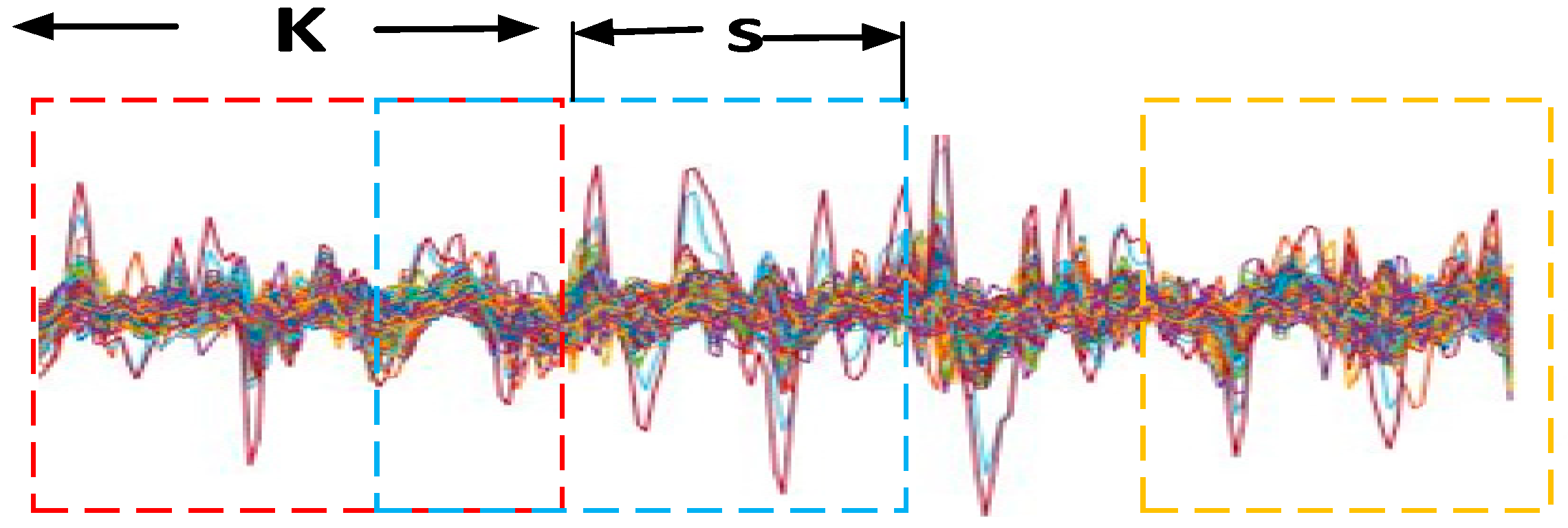
Figure 3.
High-order dynamic FC construction.
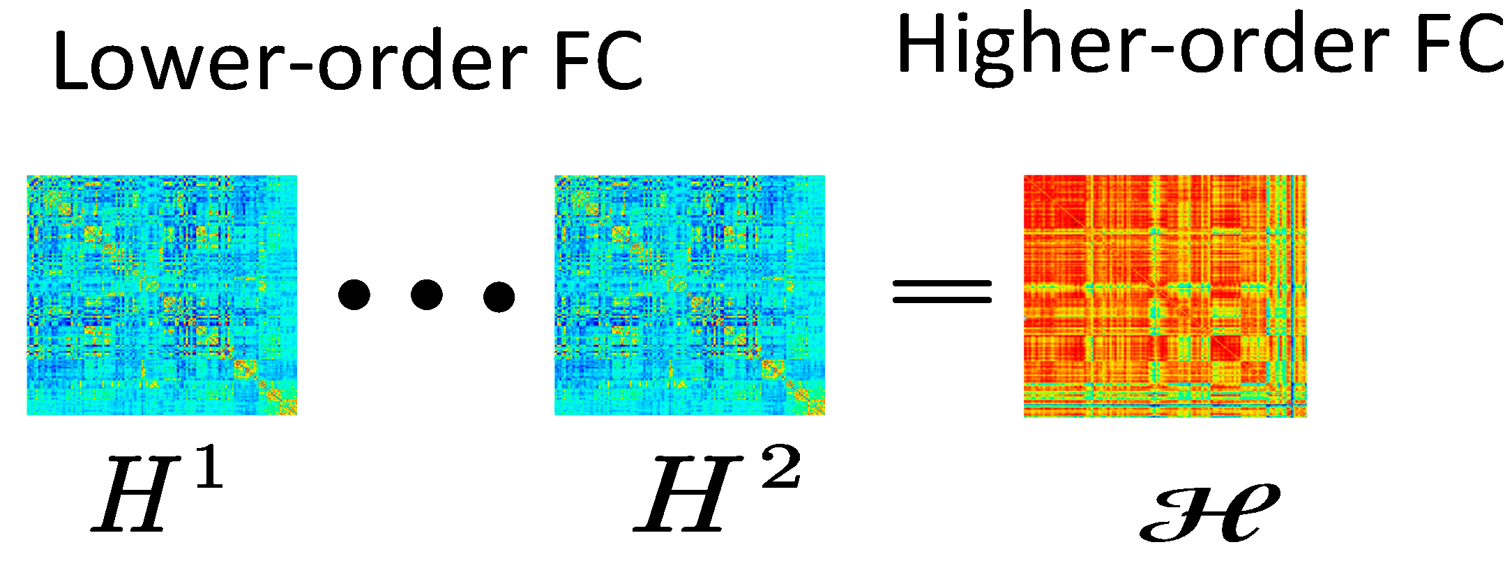
Figure 4.
Effect of step size on Classification accuracy while window length was set to 60 for different frequency bands: (a) AD vs. HC, (b) AD vs. MCI, (c) HC vs. MCI.
Figure 4.
Effect of step size on Classification accuracy while window length was set to 60 for different frequency bands: (a) AD vs. HC, (b) AD vs. MCI, (c) HC vs. MCI.
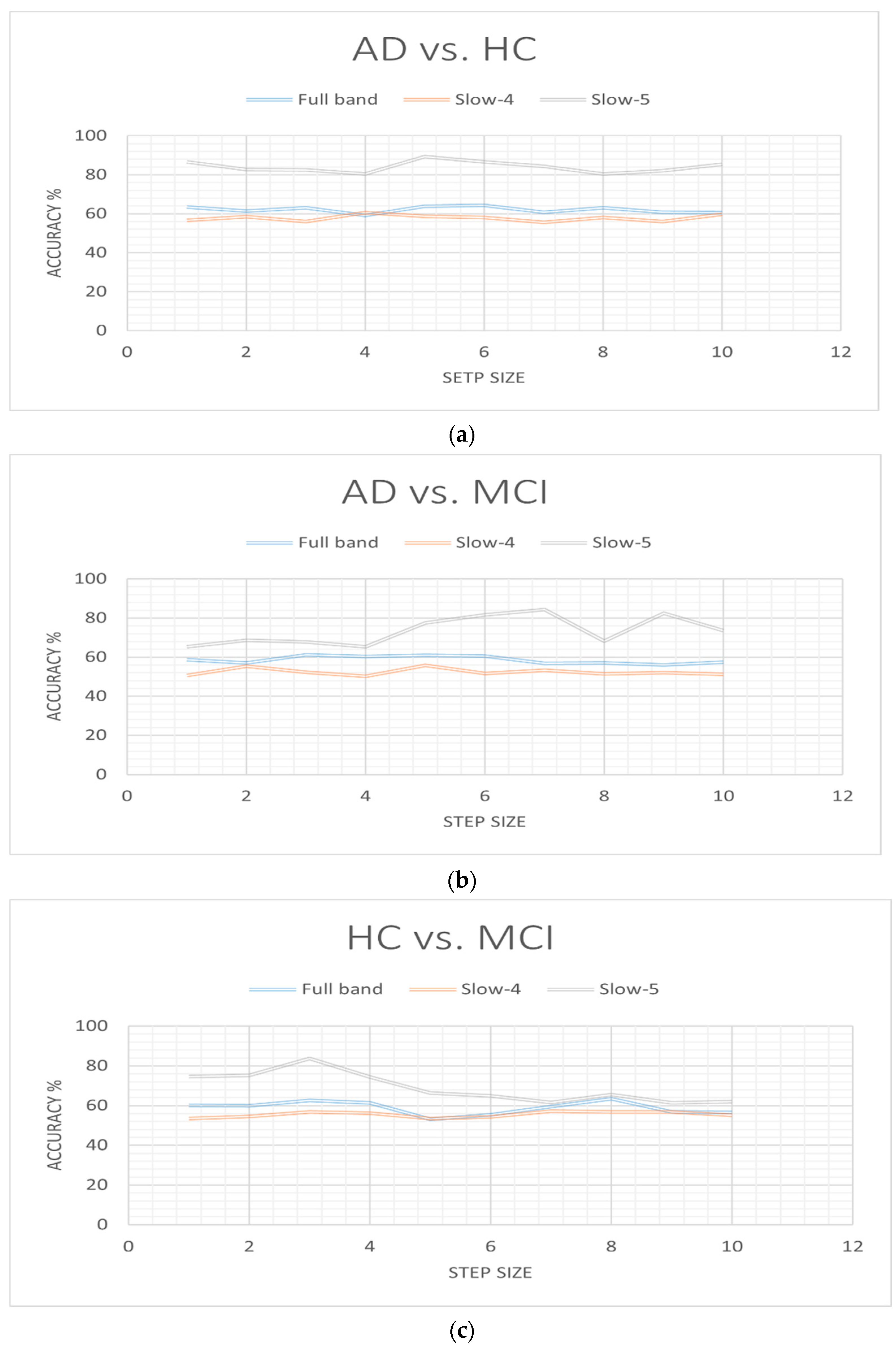
Figure 5.
ROC curve (AUC) for All frequency Band network features combination.
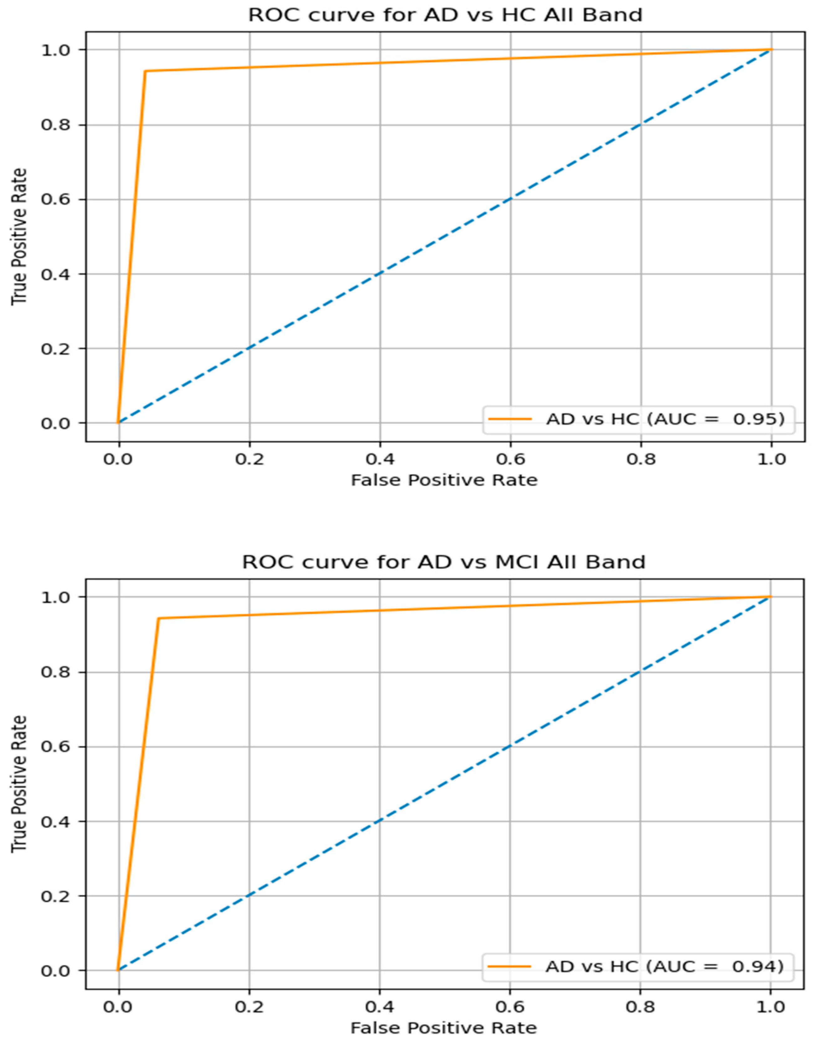

Figure 6.
Classification results at different frequency bands: (a) AD vs. HC classification performance, (b) AD vs. MCI classification performance, (c) HC vs. MCI classification performance.
Figure 6.
Classification results at different frequency bands: (a) AD vs. HC classification performance, (b) AD vs. MCI classification performance, (c) HC vs. MCI classification performance.
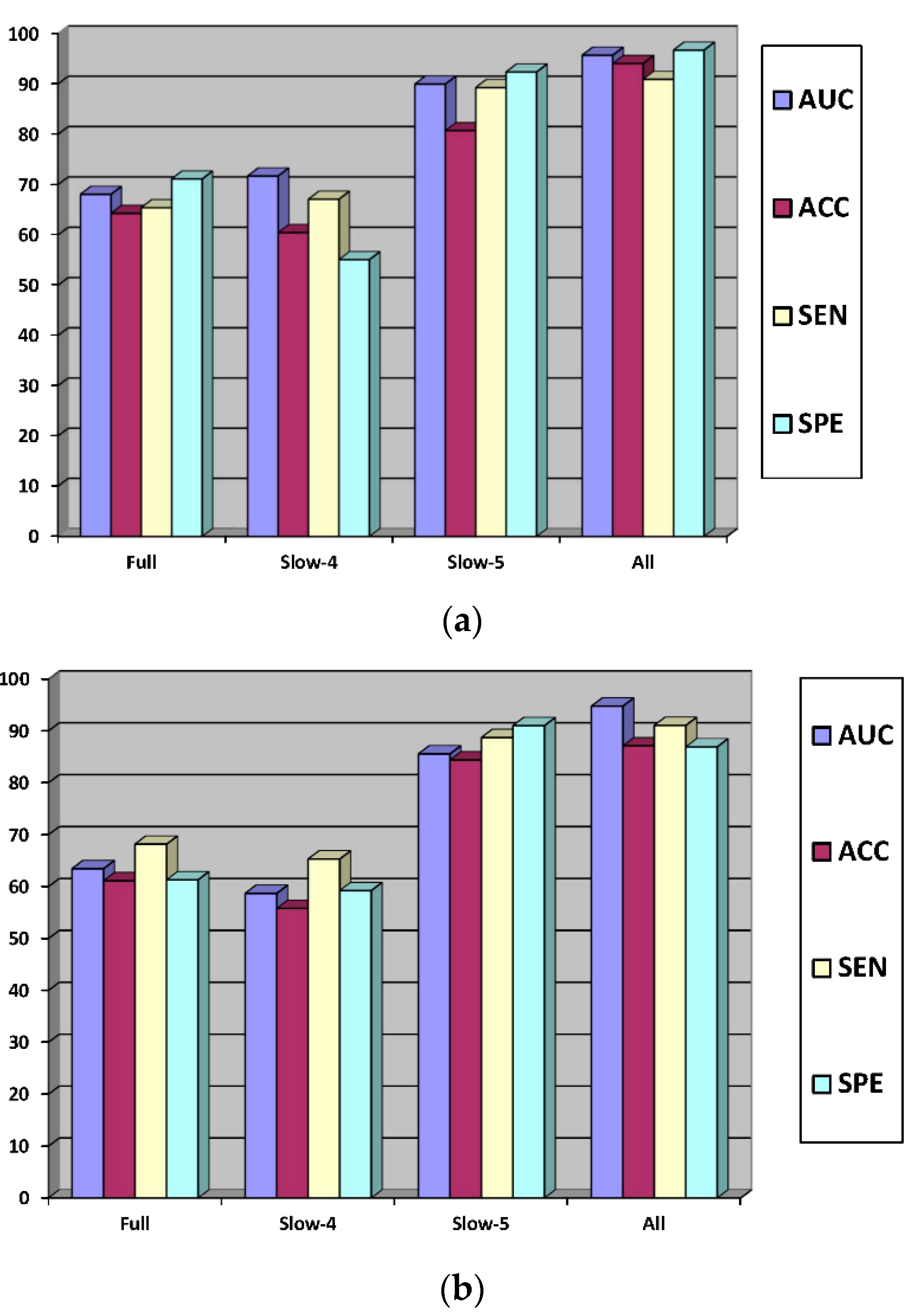
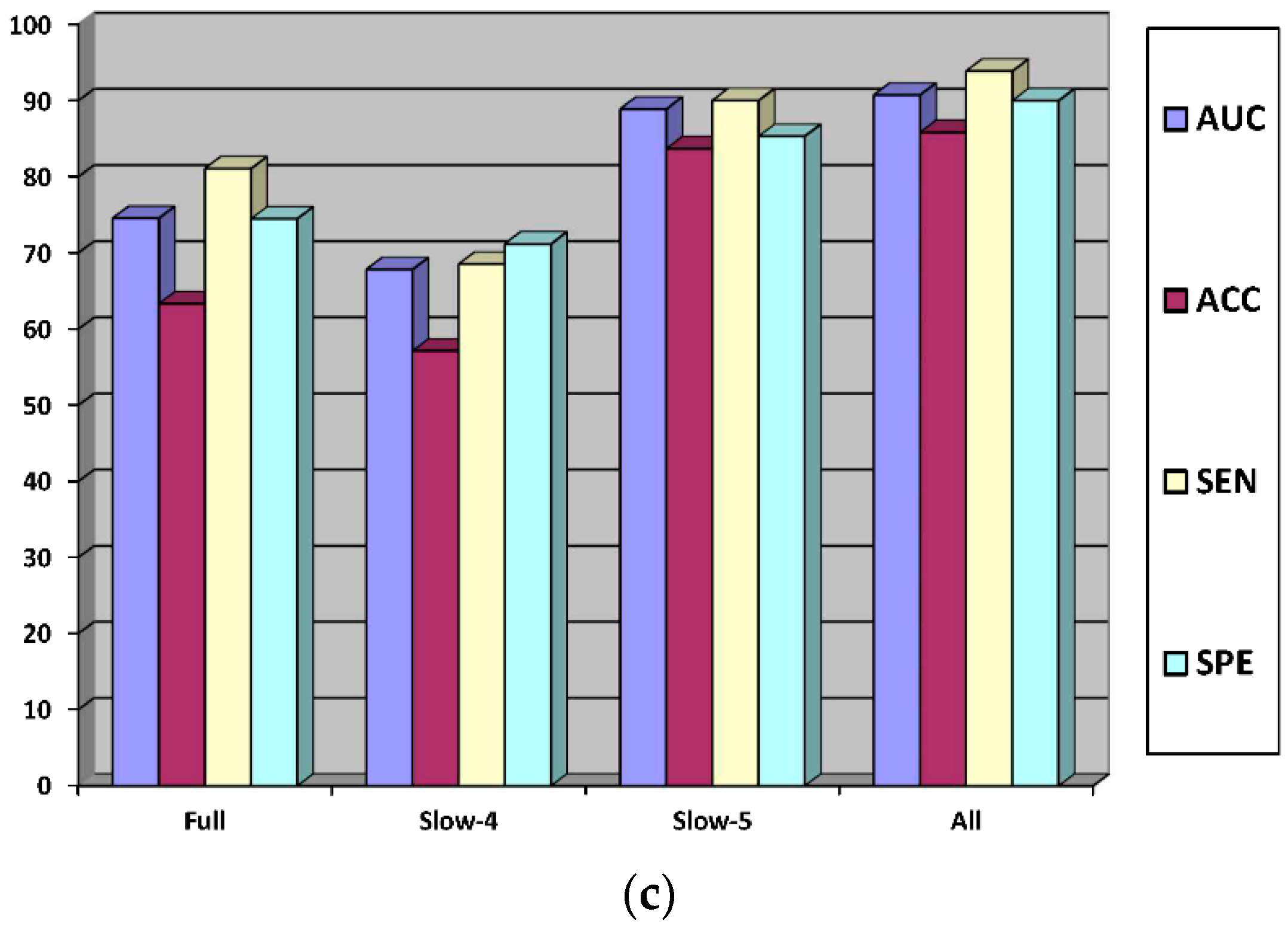
Figure 7.
Illustration of topmost selected brain regions: (a) AD vs. HC, (b) AD vs. MCI, (c) HC vs. MCI.
Figure 7.
Illustration of topmost selected brain regions: (a) AD vs. HC, (b) AD vs. MCI, (c) HC vs. MCI.


Table 1.
Demographics of the participant subjects.
| Group | MCI | AD | HC |
|---|---|---|---|
| Nos. of Subjects | 61 | 35 | 35 |
| Male/Female | 33/28 | 23/12 | 14/21 |
| Age | 72.80 ± 7.9 | 75.65 ± 8.61 | 77.83 ± 6.17 |
| FAQ score | 2.74 ± 3.71 | 4.46 ± 4.01 | 0.33 ± 0.78 |
| CDR | 0.5 | 0.7 ± 0.3 | 0 |
| MMSE score | 26.42 ± 3.75 | 19.59 ± 4.56 | 29.13 ± 1.20 |
Table 2.
Classification Results.
| Group | Frequency Band | Classifiers | AUC | ACC | SEN | SPE |
|---|---|---|---|---|---|---|
| AD vs. HC | Full band | SVM | 68.10 | 64.33 | 65.45 | 71.15 |
| Slow-4 | 71.74 | 60.50 | 67.13 | 55.12 | ||
| Slow-5 | 80.77 | 89.30 | 92.41 | 88.90 | ||
| All | 95.74 | 94.10 | 90.95 | 96.75 | ||
| AD vs. MCI | Full band | SVM | 63.45 | 61.13 | 68.17 | 61.30 |
| Slow-4 | 58.70 | 55.80 | 65.31 | 59.23 | ||
| Slow-5 | 85.57 | 84.40 | 88.71 | 91.01 | ||
| All | 94.77 | 87.14 | 91.05 | 86.91 | ||
| HC vs. MCI | Full band | SVM | 74.57 | 63.35 | 81.09 | 74.50 |
| Slow-4 | 67.85 | 57.17 | 68.54 | 71.20 | ||
| Slow-5 | 88.90 | 83.71 | 90.03 | 85.33 | ||
| All | 90.75 | 85.85 | 93.89 | 90.01 |
AD = Alzheimer’s disease; HC = Healthy Control; MCI = Mild Cognitive Impairment; SVM = Support Vector Machine; AUC = Area Under Curve, ACC = Accuracy; SEN = Sensitivity; SPE = Specificity.
Table 3.
Comparison with existing state-of-art method.
| Reference | Methods | No of Subjects | Group | ACC | SEN | SPE |
|---|---|---|---|---|---|---|
| Challis et al. [39] | Covariance, 82 ROIs, logistic regression, Bayesian Gaussian Process | 20 HC/50 MCI/27 AD | AD vs. MCI | 0.8 | 0.7 | 0.9 |
| MCI vs. NC | 0.75 | 1.00 | 0.5 | |||
| de Vos et al. [40] | Amplitude of low frequency fluctuation | 173 HC/27 AD | 0.76 | 0.71 | 0.82 | |
| Sparse partial correlation FCNs, 70 ROIs | 0.75 | 0.79 | 0.71 | |||
| Sparse partial correlation dynamic FCNs, 70 ROIs | 0.78 | 0.83 | 0.73 | |||
| khazaee et al. [10] | graph measure | 20 AD/20 HC | AD vs. HC | 90.00 | ||
| Our method | HoD-FCN (Full band, slow-4, slow-5) | 35 HC/61 MCI/35 AD | AD vs. HC | 94.1 | 90.95 | 96.75 |
| AD vs. MCI | 87.14 | 91.05 | 86.91 | |||
| HC vs. MCI | 85.85 | 93.89 | 90.01 |
Publisher’s Note: MDPI stays neutral with regard to jurisdictional claims in published maps and institutional affiliations. |
© 2022 by the authors. Licensee MDPI, Basel, Switzerland. This article is an open access article distributed under the terms and conditions of the Creative Commons Attribution (CC BY) license (https://creativecommons.org/licenses/by/4.0/).
Share and Cite
MDPI and ACS Style
Khatri, U.; Kwon, G.-R. Classification of Alzheimer’s Disease and Mild-Cognitive Impairment Base on High-Order Dynamic Functional Connectivity at Different Frequency Band. Mathematics 2022, 10, 805. https://doi.org/10.3390/math10050805
AMA Style
Khatri U, Kwon G-R. Classification of Alzheimer’s Disease and Mild-Cognitive Impairment Base on High-Order Dynamic Functional Connectivity at Different Frequency Band. Mathematics. 2022; 10(5):805. https://doi.org/10.3390/math10050805
Chicago/Turabian StyleKhatri, Uttam, and Goo-Rak Kwon. 2022. "Classification of Alzheimer’s Disease and Mild-Cognitive Impairment Base on High-Order Dynamic Functional Connectivity at Different Frequency Band" Mathematics 10, no. 5: 805. https://doi.org/10.3390/math10050805
Note that from the first issue of 2016, this journal uses article numbers instead of page numbers. See further details here.