
Bistability and Chaos Emergence in Spontaneous Dynamics of Astrocytic Calcium Concentration
by
 , , and
Evgeniya V. Pankratova
1,2,* ,
,
Maria S. Sinitsina
1,
Susanna Gordleeva
1,3 and
Victor B. Kazantsev
1,2,3 1
Lobachevsky State University of Nizhni Novgorod, 603950 Nizhny Novgorod, Russia
2
Neuroscience Research Institute, Samara State Medical University, 443099 Samara, Russia
3
Neuroscience and Cognitive Technology Laboratory, Center for Technologies in Robotics and Mechatronics Components, Innopolis University, 420500 Innopolis, Russia
*
Author to whom correspondence should be addressed.
Mathematics 2022, 10(8), 1337; https://doi.org/10.3390/math10081337
Submission received: 3 March 2022
/
Revised: 9 April 2022
/
Accepted: 12 April 2022
/
Published: 18 April 2022
(This article belongs to the Section Mathematical Biology)
Abstract
:In this work, we consider a mathematical model describing spontaneous calcium signaling in astrocytes. Based on biologically relevant principles, this model simulates experimentally observed calcium oscillations and can predict the emergence of complicated dynamics. Using analytical and numerical analysis, various attracting sets were found and investigated. Employing bifurcation theory analysis, we examined steady state solutions, bistability, simple and complicated periodic limit cycles and also chaotic attractors. We found that astrocytes possess a variety of complex dynamical modes, including chaos and multistability, that can further provide different modulations of neuronal circuits, enhancing their plasticity and flexibility.
Keywords:
spontaneous calcium oscillation in astrocytes; mixed-mode oscillations; bistability; chaosMSC:
34C15; 34C23; 34C28; 34C60; 37N25; 92B251. Introduction
Recent experimental and theoretical findings demonstrated that glial cells, particularly astrocytes, can participate in neuronal signaling and brain information processing. Astrocytes operate at the time scale of seconds and can release different gliotransmitters, e.g., neuroactive chemicals, modulating neuronal activity from the level of single synapses up to coordination of different networks. Chemical calcium excitability represents the characteristic feature of astrocytic signaling [1,2,3,4,5,6,7,8]. Ca elevations in astrocytes are vital for the optimal functioning of the CNS [9]. Astrocytic Ca signals also control K uptake [10], contribute to the regulation of local blood flow [11] and morphological plasticity of these cells [12] and induce the release of gliotransmitters [13]. It is believed that this release which is crucial for neuronal regulation is directly connected with the generation of intrinsic calcium pulses. That is, the calcium signals and their characteristics further define synaptic transmission efficiency and, hence, the dynamics of the accompanying neuronal networks.
Astrocytes display both triggered and spontaneous calcium signals. Spontaneous Ca events are generated intrinsically without any external stimuli, whereas triggered calcium events occur in response to changes in the astrocytic environment, such as synaptic or neuronal activity and physiologically relevant internal and external triggers. The mechanisms underlying the generation of spontaneous Ca elevations in astrocytes are still poorly understood [14]. In experiments, it was shown that astrocytes can generate spontaneous calcium signals during blocking the neuronal activity [15], blocking vesicular release from neurons and astrocytes [16,17] and, in the case of inositol 1,4,5-trisphosphate receptor type 2 (IP3R2), genetic deletion in astrocytes [18,19]. However, genetic knockout of IP3R2 leads to a considerable reduction of spontaneous calcium events supporting the importance of the endoplasmic reticulum (ER) and the IP3R.
Many experimental works show complex behavior of spontaneous calcium signaling in astrocytes which can vary from periodic pulses to irregular oscillations [16,20,21]. However, in these studies no mechanism was proposed for how the different modes of behavior emerged. The theoretical analysis of detailed biologically relevant models of calcium activity in astrocytes similar to that carried out in the present work can help investigate more precisely the principles of complex calcium oscillations emergence and characterize in more detail the transitions between different regimes of dynamical behavior, i.e., periodic oscillations, bursting, bistability, and chaos. In contrast to those for neuronal dynamics, studies for astrocytic calcium activity were carried out to a much lesser extent. For example, multistability in the dynamics of a single neuron is characterized by the coexistence of basic signaling regimes, such as quiescent mode, regular spiking, and chaotic bursting [22]. The phenomenon of the transition between the different dynamical modes under the influence of noise is interpreted as a dynamic short-term memory [23]. Numerous diverse dynamical regimes in neuronal interactions have also been examined both theoretically and experimentally [24] and are thought to play an important role in neural system signaling [25]. It is believed that on the neural network level, multistability is the basic mechanism for associative memory formation and pattern recognition [25]. The proposed mechanism postulatesthat the neural network dynamical modes that correspond to different brain states representing specific perception objects can be switched by applying some input independently on changing parameters.
Recent experiments showed that spontaneous calcium transients are mediated by stochastic Ca fluxes through diverse pathways [14]. Calcium is able to enter the astrocyte through the plasma membrane (via Na/Ca exchanger, Ca-permeable receptors and channels) or can be released by mitochondria via a stochastic opening of IP3Rs on the ER [19,26,27]. Acting together, these small Ca fluxes result in oscillations of the cytosolic Ca concentration that can exceed the threshold for Ca-dependent Ca release (CDCR) through IP3Rs, leading to the gain of spontaneous Casignals. Elevations of cytosolic Ca can also enhance IP production via activation of the delta-isoform of phospholipase C (PLC) [28]. The cytosolic concentrations of IP and Ca jointly control the opening probability of IP3Rs [29], and a high IP level increases the chance of spontaneous Ca transients becoming amplified through CDCR. Despite the experimental studies into this area, cellular and molecular mechanistic details underlying spontaneous Ca events in astrocytes have not yet been fully clarified.
Several mathematical models have been proposed for the generation of this type of Ca oscillations. These computational studies offer different molecular mechanisms of how spontaneous Ca signals arise in astrocytes, such as the flux of extracellular Ca across the plasma membrane into the cytosol [27,30,31], spontaneous IP production mediated by PLC [32], or the diffusion of IP through gap junctions [33,34,35]. For a recent review of the state-of-the-art in computational modeling of calcium signaling and dynamics in astrocytes see [36].
In this study, we investigated the impact of key intracellular Ca and IP pathways on the generation of spontaneous Ca oscillations in astrocytes using bifurcation theory and numerical simulation. For this, we investigated a mathematical model of spontaneous Ca activity in astrocytes which displays physiologically plausible oscillatory behaviors [31]. Within this model, spontaneous Ca events were triggered by small changes in cytosolic Ca levels that were caused by Ca entry through the plasma membrane, Figure 1. Ca oscillations emerged due to interplay of two feedback loops involving changes in intracellular Ca and IP concentrations. The feedback loops control the release of Ca from the ER to the cytosol through the IP3R2. The first feedback loop consists of IP3Rs open probability modulation by cytosolic Ca. The other one is determined by the fact that the Ca dependent PLC activation results in IP production, which, in turn, enhances the CDCR. We used modern tools of bifurcation theory to characterize the dynamics of astrocytic IP and Ca depending on variation of the key kinetics constants of the pathways used by Ca for entry and exit to the ER and IP production by PLC. We focused on key bifurcation scenarios of transitions between different dynamical modes of calcium signaling including the appearance of multistability and chaotic calcium oscillations.
The outline of the paper is as follows. In Section 2, we describe the considered mathematical model. In Section 3, we focus on the role of an input calcium flow and examine the properties of the regimes observed for the spontaneous calcium concentration. The coexistence of different regimes is discussed in Section 3.2. The role of the output calcium flow in the emergence of complicated regular and irregular mixed-mode oscillations of calcium concentration is studied in Section 4. In Section 5, compliance with experimental data and astrocytic chemical activity contribution to information processing are discussed. Finally, Section 6 summarizes the conclusion.
2. Description of the Mathematical Model
The Lavrentovich–Hemkin [31] model describes the dynamics of the intracellular calcium concentration and Ca-dependent concentration of inositol-1,4,5-triphosphate (IP), by the following three-dimensional dynamical system:
where the expressions for , and are:
Dynamical variables include the intracellular calcium concentration , the calcium concentration in the internal storage endoplasmic reticulum (ER), and the concentration of the secondary messenger inositol-1,4,5-triphosphate , which controls the ionic channels and removes calcium into the cytosol. Most of the parameters of the system (1) were chosen according to the data of [31]: M/s, , M/s, M, M, M, M, M, , , , , . Note that in [31], the authors provided the computational simulation of conditions carried out in real experimental studies and illustrated the dynamics that were qualitatively similar to the experimental data. With this aim, the authors demonstrated the impact of the influx of the Ca ions from the extracellular matrix on both (i) the period change of the regular spontaneous calcium oscillations in astrocytes and (ii) the complicated dynamics appearance. In [30], the authors expanded this system of nonlinear differential equations by combining it with different types of voltage-gated calcium channels. At the same time, the mechanisms responsible for the change of the regimes still remained incomprehensible. To our knowledge, refs. [37,38,39] are the first works with the strict analysis of the Lavrentovich–Hemkin model. Independently, the authors of both groups were interested in the bifurcation mechanisms of the spontaneous calcium oscillatory dynamics emergence and studied the peculiarities of Andronov–Hopf bifurcations in the model. Furthermore, for both scientific groups, the chaotic dynamics in spontaneous calcium oscillations had become the subject of close attention. As a result, in [40], the authors studied ways to control such complicated behavior as well as in [41], the authors demonstrated that even small changes in the parameters of the system can significantly modify the bifurcation diagram, revealing the absence of complicated oscillations.
In this work, particular attention was paid to the influence of the parameters controlling transmembrane calcium transport. In particular, we focused on the role of extracellular calcium flow and the rate of the calcium escape on the change of calcium dynamics. Additionally, the following parameters were also varied: the rate of calcium flow through serca to the ER from the cytosol, , the rate of calcium flow through IP from the ER to the cytosol, , and the amount of feedback between calcium in the cytosol and IP and , Figure 1. In contrast to previous works, in this study, we focused on the emergence of bistable behavior in spontaneous calcium dynamics and on the ways for the emergence of various types of chaotic dynamics. In our calculations, the system of nonlinear differential equations (1) was numerically solved by the fourth order Runge–Kutta integration scheme with a time step of 0.005 s. To study the peculiarities of transition from the steady state solution to the oscillatory mode, different one- and two-parametric diagrams were calculated. In all calculations to obtain more accurate results; the transients were discarded. To study various chaotic regimes, we calculated the largest Lyapunov exponent by the use of the numerical method introduced by Wolf et al. [42].
3. Input Calcium Flow
Let us start from the parameter set considered in the original paper by Lavrentovich and Hemkin in [31]. For this case, weak flow of an extracellular calcium through the astrocytic membrane leads to a steady state regime at which the concentration of calcium in the ER can exceed the concentration of calcium in the cytosol by tens of times. As illustrated in Figure 2a, for M/s, for instance, at the time s the concentration of M and M. Meanwhile, concentration in the cell approaches M. The increase of leads to the appearance of oscillations in the system dynamics. Particularly, from the data obtained for M/s, Figure 2b, it follows that decreasing the phase of during the oscillatory mode provokes a sharp increase in both and up to the values of M and M, respectively. Following the increase of leads to another steady state regime at which the concentrations of calcium in the ER and in the cytosol weakly differ. For M/s, Figure 2c, at the time s these concentrations differ by four times only, M and M, respectively.
Note that, a twofold decrease of ( instead of ), Figure 2d–f, had little effect on the dynamical regimes observed in the system. This just led to a slight change in the period and the amplitude of the oscillatory mode, Figure 2e, and to a slight change of the concentrations of at the steady states, Figure 2d,f in comparison with Figure 2a,c, respectively. As we will strictly demonstrate further, any changes of do not impact the concentrations of and at the steady states.
An additional fivefold decrease of (M/s instead of M/s) led to the shift of oscillatory mode appearance to larger values of . Similar to the previous cases for M/s, the steady state was observed. For this steady state, both and were changed in comparison with Figure 2a, while the value of was not changed for the constant . For M/s, the system demonstrated the oscillatory mode with a large period. Moreover, for this oscillatory regime, more than a twofold increase of the maximal calcium concentration in the endoplasmic reticulum was observed. For example, M/s approached the value M as shown in Figure 2i (for instance, in Figure 2b, increased only up to the value M, and in Figure 2e, up to M). Note that the period of oscillations shown in Figure 2i was even larger than in Figure 2e.
3.1. Steady States and Oscillatory Modes
To illustrate the peculiarities of the transition from steady state mode to oscillatory regime, Figure 3a–i show the two-parametric bifurcation diagrams. To present the whole dynamical picture, all three variables of the considered system were studied. The diagrams shown in the first column of Figure 3 were obtained for , the results for are presented in the middle column, and the right column shows the diagrams obtained for . The calculations were carried out for the parameters , , , and . Different shades of blue show the values of the system variables within the quiescent modes. The darker tone of blue corresponds to larger values of the corresponding concentrations. As seen from the diagrams, the concentration of calcium in the cytosol is always increased with the growth of extracellular calcium flow through the astrocytic membrane. In Figure 3a,d,g, the darker tone of blue is observed for larger values of . The law for this growth can be obtained analytically by equating the right parts of the system (1) to zero (see Appendix A for details):
where
As follows from (2), the steady state concentration of calcium in the cytosol depends on only two parameters, and . Thus, the increase of leads to the linear growth of as seen in Figure 3a,d,g.
A similar change in the dynamics of concentration can also be observed in Figure 3c,f, where the increase of provides the monotonous growth of the steady state concentration for any values of and , respectively. Indeed, it follows from (5), that the nonlinear law for this growth is: , where . Since its derivative is positive for any , equality (5) is the monotonously increasing function. Similar analysis of the Formula (5) allows us to explain the diagram shown in Figure 3i. Here, the increase of leads to the corresponding scaling only: larger values of give larger values of .
From the diagrams shown in Figure 3b,e,h, it follows that, for , a more complicated behavior is observed. As expected, the larger values of (the rate of calcium flow through serca to the ER from the cytosol) lead to larger concentrations of . In contrast, for a larger value of (the rate of calcium flow through IP from the ER to the cytosol), the smaller steady state value of is observed. Indeed, from equality (3), it follows that and .
Note that for small input calcium flow , particularly, for M/s, it seems that the level of the calcium concentration in the endoplasmic reticulum does not depend on , especially for the diagrams shown in Figure 3e,h. However, that is not the case. It can easily be shown that for small , is small enough, and equality (5), therefore, yields
revealing that (i) -dependence increases nonmonotonously (its derivative increases with the increase of ) and () both parameters, and do not change the value of calcium concentration in the endoplasmic reticulum.
Thus, the analysis of the steady state domains shows that two ranges in can be contingently highlighted: One range is for before the oscillatory mode (for small ), and the other is after it (for large ). Within these ranges, the intracellular calcium and concentrations are different. Moreover, within these ranges, the ER calcium concentration even changes differently.
In the oscillatory regime, the difference between the minimal and the maximal value of the corresponding variable is shown by shades of red. Thus, the domains with a red-to-yellow gradient present the parameter-dependent evolution of , , and , respectively. In this case, the darker tone of red corresponds to larger values of the corresponding difference. From Figure 3a–c, it follows that the increase of leads to an increase of all the considered differences , , and . Moreover, an analysis of the oscillatory solutions calculated for various showed that the increase of this parameter also leads to the increase of the maximal values of all variables and to the significant growth of the oscillations period. For the considered range of the parameter , the difference (together with the maximal value of the corresponding variable) monotonously grows with the increase of . Meanwhile, and demonstrate nonmonotonous behavior with the increase of , Figure 3e,f. Analysis of the solutions calculated for various showed that the increase of this parameter leads to the increase of (as well as the maximal values of ), while and are decreased. Moreover, with the increase of , the period of oscillations is also decreased.
Note that for small values of the considered parameters , , and , for any value of the external calcium concentration , only a steady state regime can be observed. Thus, only for the parameters exceeding certain threshold values , , and , the emergence of an oscillatory mode is possible.
Particular attention should be paid to the analysis of the system behavior near the boundaries between the regions with steady states and oscillatory modes, i.e., between the domains shown in Figure 3 by the gradients of blue and red(yellow). It was shown that the nature of the equilibrium point stability change can be different near the different parts of this boundary. To further show the peculiarities, we consider Figure 3a in more detail.
3.2. Bistability Emergence: Coexistence of Steady State and Oscillatory Mode
Examining the diagram shown in Figure 4a, we focus on a particular value of the parameter . Namely, for M/s, we have two values of defining the transition from one domain to another. Figure 4b,c present time series calculated for all three variables of the system and parameter taken close to the upper boundary of the oscillatory domain, i.e., for M/s. Figure 4b was obtained for initial conditions , Figure 4c is for initial . In Figure 4d,e, the coexisting solutions near the lower boundary (for M/s) are demonstrated. Figure 4d was obtained for initial conditions , Figure 4e is for initial . Thus, for spontaneous calcium dynamics, the multistability being the crucial in sudden switchings of the dynamical regimes [43,44,45,46,47], is also possible.
To show the change of amplitude in oscillatory mode, we calculated the differences (blue solid line) and (green dashed line) with the change of , Figure 4g. In comparison with Figure 3a,c, such differences in oscillatory mode are observed for the section considered at M/s with the change of the parameter .
To obtain the width of the ranges with bistable dynamics, we focused on only. Near both boundaries of the oscillations-to-quiescence transition, the calculations were performed twice. Namely, for the lower boundary, the calculations of with the increase of the parameter were carried out using the initials in a vicinity of the steady state (blue solid line in Figure 4f). These initials can be obtained automatically because for small , the steady state is globally stable (due to its uniqueness). Therefore, in numerical calculations, small changes in with taking the initials in the steady state observed for the previous value of , provide the initials within the small vicinity of the shifted steady state. The calculations of with the decrease of the parameter were carried out by using the initials in a vicinity of the limit cycle (orange dashed line in Figure 4f). Here, for large enough values of (but still close to the boundary), the limit cycle is a unique attracting set in the phase space of the system. Thus, the initials near the limit cycle with the small change of can be obtained automatically.
Similarly, for the upper boundary, the calculations of with the increase of the parameter were carried out using the initials in a vicinity of the limit cycle (blue solid line in Figure 4h). In contrast, the calculations of with the decrease of the parameter were carried out using the initials in the vicinity of the steady state (orange dashed line in Figure 4h). Thus, the width of the ranges with the bistable type of behavior is M/s and M/s for the lower and upper boundaries, respectively.
Obviously, the equilibrium point stability is lost via subcritical Andronov–Hopf bifurcations leading to the birth of unstable limit cycles near the red points depicted in Figure 4f,h. Note that this result is consistent with theoretical studies reported in [38]. For the lower boundary, the increase of the unstable cycle amplitude with the decrease of occurs, while for the upper boundary, the unstable cycle amplitude is increased with the increase of . Approaching the stable limit cycles, both unstable cycles collide with the latter and disappear via fold limit cycle bifurcations at M/s and M/s, respectively.
Taking into account the numerical results presented above, we can summarize the following proposition.
Proposition 1.
For the Lavrentovich–Hemkin model with the parameters taken as in [31]:
- (a)
- The change of extracellular calcium flow reveals the existence of two -values where the Andronov–Hopf bifurcation occurs;
- (b)
- Both the Andronov–Hopf bifurcations are subcritical, i.e., the change of the equilibrium stability occurs with an unstable limit cycle emergence;
- (c)
- These unstable limit cycles coalesce with the stable cycles and disappear via the fold limit cycle bifurcations with further change of extracellular calcium flow. The -parameter ranges between the Andronov–Hopf and the fold limit cycle bifurcations define the ranges of bistability, where the coexistence of an oscillatory and steady state modes is observed.
Note that for small values of , the transition from the steady state mode to the oscillatory regime occurs via the supercritical Andronov–Hopf bifurcation [48]. Here, the emergence of small amplitude oscillations is observed, and the boundary crossing corresponds to a transition from one monostable regime to another.
4. Output Calcium Flow
Similarly to the analysis given in Section 3, the peculiarities of transition from steady state mode to oscillatory regime were also examined for the parameters , and , and .
4.1. Steady States and Oscillatory Modes
Figure 5a–i present two-parametric bifurcation diagrams calculated for all three variables of the considered system: , , and . Different shades of blue show the values of the system variables within the quiescent modes. The domains with the red-to-yellow gradient show the differences (Figure 5a,d,g), (Figure 5b,e,h), and (Figure 5c,f,i). Here, for , the darker tone of color is observed for smaller values of because from equality (2), it follows that .
For , in Figure 5c,f, the increase of provides the monotonous decrease of the steady state concentration for any values of and , respectively. Indeed, it follows from (5) that the nonlinear law for this decrease is , where . This means that for any values of parameters and , equality (5) defines the monotonously decreasing function because its derivative is negative for any > 0. A similar analysis of Formula (5) allows us to explain the diagram shown in Figure 5i. Here, the increase of leads to the corresponding scaling only; larger values of give larger values of .
From the diagrams shown in Figure 5b,e,h, it follows that for , more complicated behavior is observed. As expected, the larger values of lead to larger concentrations of , while the larger values of , in contrast, lead to a smaller steady state value of . Indeed, from (3), it follows that and . For small values of , a high level of the calcium concentration in the endoplasmic reticulum is observed.
In an oscillatory regime, as in Section 3, the difference between the maximal and the minimal value of the corresponding variable is shown by the gradient of red-to-yellow. The darker tone of the red in the two-parametric diagrams Figure 5a–i corresponds to larger values of the corresponding difference. From Figure 5a–c, it follows that the increase of leads to an increase of all the considered differences , , and . Moreover, analysis of the oscillatory solutions calculated for various showed that the increase of this parameter also leads to the increase of the maximal values of all variables and to the significant growth of the oscillation period. For the considered range of the parameter , the difference (together with the maximal value of ) monotonously grows with the increase of . Meanwhile, and demonstrate nonmonotonous behavior with the increase of , Figure 5e,f. Analysis of the solutions calculated for various showed that the increase of this parameter leads to the increase of (as well as the maximal values of ), while and are decreased. Moreover, with the increase of , the period of oscillations is also decreased.
4.2. Chaotic Spontaneous Calcium Dynamics
From the experimental data, it follows that a peculiarity of astricytic chemical activity is in the presence of peaks with different amplitudes of calcium concentration. In accordance with terminology given in [49], blips are short and weak peaks that correspond to the opening of one IP3R channel (or one tetramer in an IP3R channel), while the puffs are longer and higher peaks resulting from the coordinated opening of a group of neighboring IP3R channels (or their tetramers) through the calcium-induced calcium release principle (CICR). The emergence of complicated alternations of such peaks is possible within the framework of the Lavrentovich–Hemkin mathematical model [31]. Furthermore, we present three types of chaotic spontaneous elevation of astrocytic calcium.
4.2.1. Burst-Type Dynamics: Small-Peaks Irregularity
Note that in [31], the authors presented an example of complicated calcium dynamics that can emerge with the change of an extracellular calcium level. To obtain such complicated chemical activity, few parameters were changed in the model. Namely, the authors considered the case when M (instead of M) and M (instead of M). Physically, these changes of the parameters correspond to the situation where the dynamics have a faster response to Ca in astrocytic cytoplasm, while the rate of calcium release via the IP3R (through the CICR) occurs at a higher concentration of cytosolic calcium, and this rate would not drop off as quickly. Using the same assumptions, we consider the parameters as in [31] and study the role of the output calcium flow in the emergence of chaotic chemical activity.
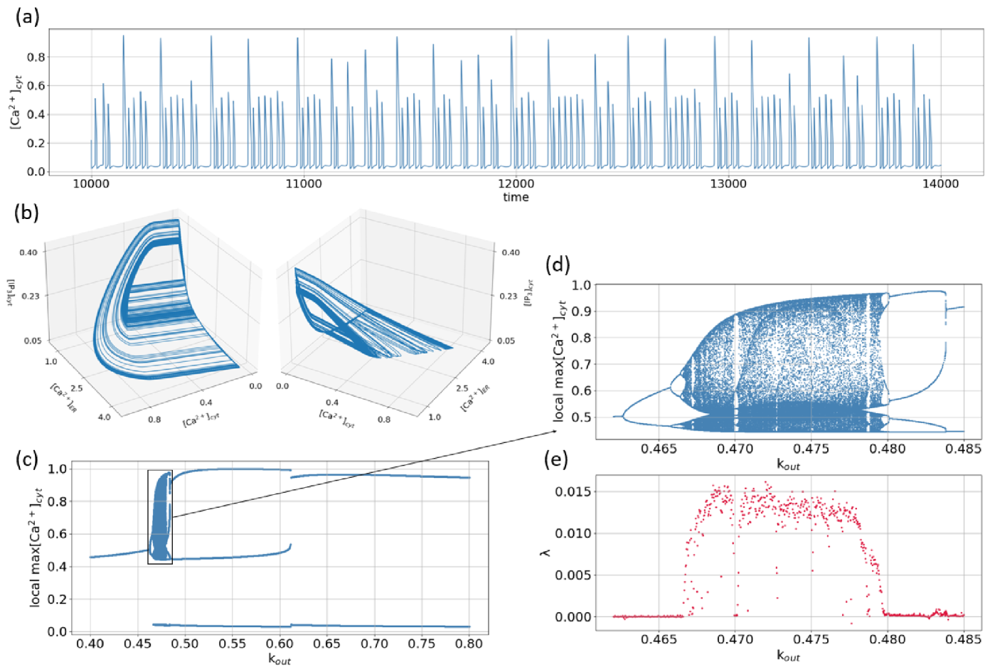
Figure 6a,b show an example of irregular time series numerically obtained for the concentration of the cytoplasmic calcium and 3D pictures of the corresponding attractor in the phase space of the system (1), respectively. As seen from the time series, being on this attractor, the phase point returns on a large amplitude loop after different time intervals defined by the time spent in the region of low-amplitude oscillations. Such activity looks like bursts with various durations of small-amplitude, during which the amplitude is chaotically varied. It is remarkable that such types of bursting or mixed-mode oscillations are quite widespread in nonlinear neurodynamical systems [50,51,52,53,54,55,56,57,58]. Note that for the parameters taken in Figure 6a,b, the equilibrium state being a saddle with the eigenvalues and , is located in the point .
To study the dynamical mechanism leading to emergence of the attractor shown in Figure 6a, the one-parametric bifurcation diagram was obtained. As a control parameter, the rate of the output calcium flow was considered. For each value of taken from the interval , the local maximums of -dependence were plotted on the diagram, Figure 6c. It should be noted that, simple limit cycle with local maximum located near M (for small ), disappears with the following decrease of (for the steady state can be obtained).
As seen from the enlarged part of the diagram, Figure 6d, with the increase of , the period-doubling cascade is observed. As a result of such a bifurcation scenario, a chaotic small-amplitude attractor emerges in the phase space of the system (not shown, but similar oscillations were observed, for instance, with the change of in [37] or in [41]). A further increase of leads to the appearance of a large-amplitude loop, and the attractor becomes similar to that shown in Figure 6a. On the bifurcation diagram, this corresponds to the appearance of an upper line for . As seen from the enlarged part shown in Figure 6d, the change of within the interval leads to the appearance of several alternating periodic windows and chaotic bands. The observed transitions are well characterized by the maximal Lyapunov exponent shown in Figure 6e.
With a further increase of , only periodic mixed-mode oscillations take place. The evolution of such oscillations can be described by the use of the notation with and being the integers indicating the numbers of large (puffs) and small (blips) maximum values of oscillations in one period, respectively. Thus, for , the following sequence can be written: . Note that contrasting similar transitions can be obtained with the decrease of the input calcium flow [31].
4.2.2. Small-Amplitude Chaotic Chemical Activity
Considering the smaller value of the parameter , e.g., M, here we examine the peculiarities of astrocytic chemical activity when the dynamics have an even faster response to Ca in astrocytic cytoplasm than it was assumed in the previous case. For , Figure 7a,b show an example of irregular time series numerically obtained for and 3D pictures of the corresponding attractor in the phase space of the system, respectively. The one-parametric bifurcation diagram was obtained for , Figure 7c.
In this case, for all the considered interval of , the large amplitude loop does not appear. As seen from Figure 7d, the increase of the control parameter leads to the period-doubling cascade resulting in the emergence of chaos. Positive values of the maximal Lyapunov exponent shown in Figure 7e confirm the observed transitions. Distinctive features of the observed chaos are relatively small maximal values of and chaotically changed values for all its maximums. For the enlarged part of the diagram, three relatively wide periodic windows alternating with chaotic bands were obtained. In the widest window , a sequence of reverse period-doubling bifurcations yields a period-7 attractor which is later destroyed at in a crisis event. A period-5 attractor observed for the large in Figure 7d, is also destroyed in a crisis event that occurs for . For , similar to the notation used before, the following sequence can be written: .
4.2.3. Burst-Type Dynamics: All-Peaks Irregularity
Finally, we consider the case where M/s, , M, M, M. For , Figure 8a,b show an example of irregular time series numerically obtained for and 3D pictures of the corresponding attractor in the phase space of the system, respectively. The one-parametric bifurcation diagram was obtained for , Figure 8c. As for the previous case, for all the considered intervals of , the large amplitude loop does not appear. Contrary to the previous case, both an increase (from ) and a decrease (from ) of the control parameter, as seen from Figure 8d, lead to the period-doubling cascade resulting in the emergence of chaos. Positive values of the maximal Lyapunov exponent shown in Figure 8e confirm the observed transitions. For , similar to the notation used before, the following sequence can be written: .
Taking into account the numerical results presented above, we can summarize the following proposition.
Proposition 2.
Within the framework of the Lavrentovich–Hemkin mathematical model, various scenarios of chaos emergence can be realized, and therefore, various types of chaotic spontaneous calcium oscillatory dynamics in astrocytes can be simulated.
5. Discussion
Small variations in the Ca entry through plasma membrane and regimes of IP production in astrocytes can display a surprisingly rich dynamical repertoire of spontaneous Ca signaling. Keeping in mind that the astrocytic calcium induces modulations of synaptic transmission and neuronal activity, such variety of different calcium dynamics, from simple periodic oscillations to complex chaotic bursts, opens possibilities to control neuronal signaling indirectly through the neuron–astrocyte interaction.
Our study suggested several biophysical mechanisms underlying the emergence of spontaneous Ca oscillations with various amplitudes, frequencies, shapes, and other crucial features. Two important predictions follow from the model analysis hitherto discussed. The first one concerns the spontaneous Ca signal emergence in the certain range of transmembrane Ca flux values. This result is consistent with experimental findings that discovered that most spontaneous Ca events start in an optimal range of thin distal processes [27]. It was shown that the mechanism underlying such subcellular distribution of the Ca events is that the level of Ca entry through plasma membrane in astrocytic branchlets depends on their surface-to-volume ratio. Surface-to-volume ratio is highest in the distal branchlets, where Ca entry into the cytosol therefore produces the largest Ca level elevations, which then can induce CICR by activating IP3Rs. Second is the observation that it is sufficient to slightly vary IP production rates by PLC to induce dramatic changes in the subsequent Ca dynamics. This could result in the emergence of regular, self-sustained stable oscillations, bursting or chaotic. Note that chaotic oscillations of different types combining irregular pulse sequences with variable amplitudes further provide different levels of modulations of neuronal activity, both in time and in space in the context of neuron–astrocyte interaction. Consequently, they facilitate or depress particular signal transmission pathways in neuronal nets, and chaos can be viewed as a tool to enhance degrees of freedom in astrocytic modulation of neuronal signal transmission. We also note that our results are consistent with other recent theoretical studies reporting on chaotic astrocyte signaling [38,39]. In this context, the dependencies of Ca and IP oscillatory dynamics on the regime of IP production suggested different modes of stimuli encoding by astrocytes. Periodic Ca oscillations could represent a mechanism of frequency encoding. In turn, chaotic Ca signaling could perform more complex encoding, employing frequency, phase, and amplitude encoding characteristics. It follows from our analysis that chaotic oscillations are more likely to appear for large rates of IP production by PLC. Experimental studies show that the proteins PLC tether to the plasma membrane and various intracellular structures and mainly associate with the cell periphery [59]. Thus, there is overlapping in subcellular distributions of PLC and values of surface-to-volume ratio parameter, which determine the optimal level of Ca entry through the plasma membrane for the emergence of the spontaneous Ca activity in astrocytes. This evidence supports the hypothesis of the key role of PLC in the generation of the spontaneous Ca signals mediated by the Ca flux through the plasma membrane. On the other hand, our results confirm that Ca dynamics in individual astrocytes may be significantly dependent on the astrocytic morphology and spatial distribution of the cellular and subcellular components.
Spontaneous Ca events can be modulated by different external stimuli corresponding, for example, to neuronal activity and changes in the cell environment [14]. Experimental studies reveal that Ca dynamics do not simply replicate synaptic activity but are actually much more complex [60]. This may indicate that the properties of spatiotemporal Ca dynamics both spontaneous and triggered by neuronal inputs are likely to be governed by the interplay of intrinsic astrocytic cellular properties, characteristics of neuronal inputs, and environmental changes. Understanding the complex dynamic mechanisms of intracellular Ca activity has remained a major challenge and is required due to recently identified roles of astrocytic signaling in synaptic, neural network, and memory functions [13,61]. Astrocytic Ca activity contribution to information processing remains unclear. Computational models can help with this issue. It was shown that astrocytes can induce neuronal firing synchronicity and synaptic coordination [62,63,64,65], can enhance generation of information in neuronal ensembles [66,67,68,69,70], and can contribute to memory formation [71,72,73,74,75].
Abnormal astrocytic signaling can indicate pathological conditions and cause synaptic and network imbalances, leading to cognitive impairment [61]. Understanding the mechanisms underlying calcium activity in astrocytes and their role in physiological and pathological neuronal activity will open up a perspective of new therapeutic opportunities [76,77,78].
6. Conclusions
In this work, we present a variety of dynamical regimes available within the framework of the Lavrentovich–Hemkin model in a wide and meaningful region of its parameter space. We have shown that the system has a unique equilibrium point and, for this steady state, the parameter dependent laws of the variables changes were analytically obtained. We numerically determined the domains where the dynamics fall to the unique equilibrium point of the system, where the simple limit cycles are observed, and where the bistability can emerge. We have shown the variety of the observed bursting regimes of calcium oscillations and demonstrated the attractors corresponding to various types of chaotic chemical astrocytic activity. For complicated periodic bursting activity, the parameter regions with different oscillatory dynamical behaviors were classified using the notation with and being the integers indicating the numbers of large and small maximum values of chemical activity in each period, respectively. Such classification according to the periodicity of the observed mixed-mode oscillations, allows illustrating possible dynamical transitions. These transformations in chemical activity might be crucial elements used in astrocytic coding and, therefore, implied the mechanisms modifying the neuronal activity. Providing useful background information about the mechanisms of possible astrocytic activity-based coding, the results obtained in this study can be used in further simulation of neuron–astrocytic networks and might be helpful in understanding their complicated interplay.
Author Contributions
Conceptualization, E.V.P., S.G. and V.B.K.; methodology, E.V.P. and M.S.S.; software, E.V.P. and M.S.S.; validation, E.V.P. and M.S.S.; formal analysis, E.V.P. and M.S.S.; investigation, E.V.P. and M.S.S.; resources, E.V.P. and M.S.S.; data curation, E.V.P. and M.S.S.; writing—original draft preparation, E.V.P. and M.S.S.; writing—review and editing, E.V.P., S.G. and V.B.K.; visualization, E.V.P. and M.S.S.; supervision, E.V.P. and S.G.; project administration, S.G. and V.B.K.; funding acquisition, S.G. and V.B.K. All authors have read and agreed to the published version of the manuscript.
Funding
This research was supported by the Ministry of Science and Higher Education of the Russian Federation project no. 075-15-2020-808.
Institutional Review Board Statement
Not applicable.
Informed Consent Statement
Not applicable.
Data Availability Statement
The data that support the findings of this study are available from the corresponding author upon reasonable request.
Acknowledgments
We are grateful to the reviewers for their constructive comments and valuable suggestions that have helped to improve the quality of the paper.
Conflicts of Interest
The authors declare no conflict of interest.
Appendix A
Definition A1.
A solution of an ordinary differential equation is called a steady state if it is time independent.
Proposition A1.
For any values of the parameters, Lavrentovich-Hemkin mathematical model introduced in [31], has the unique steady state solution:
where
Proof.
Equating the right parts of the system (1) to zero yields:
where the expressions for and were given in Section 2. Taking into account the equality (A6), the Equation (A5) can be rewritten in the form:
that gives the value for the calcium concentration in the cytosol at the steady state:
Finally, taking into account both (A9) and (A10), one can obtain the equality for the obtaining the calcium concentration in the endoplasmic reticulum, i.e., , at the steady state:
where
□
References
- Parri, H.R.; Crunelli, V. The role of Ca2+ in the generation of spontaneous astrocytic Ca2+ oscillations. Neuroscience 2003, 120, 979–992. [Google Scholar] [CrossRef]
- Perea, G.; Araque, A. Properties of synaptically evoked astrocyte calcium signal reveal synaptic information processing by astrocytes. J. Neurosci. 2005, 25, 2192–2203. [Google Scholar] [CrossRef] [PubMed]
- Wang, X.; Lou, N.; Xu, Q.; Tian, G.F.; Peng, W.G.; Han, X.; Kang, J.; Takano, T.; Nedergaard, M. Astrocytic Ca2+ signaling evoked by sensory stimulation in vivo. Nat. Neurosci. 2006, 9, 816–823. [Google Scholar] [CrossRef] [PubMed]
- Periasamy, M.; Kalyanasundaram, A. SERCA pump isoforms: Their role in calcium transport and disease. Muscle Nerve 2007, 35, 430–442. [Google Scholar] [CrossRef]
- Wu, Y.-W.; Tang, X.; Arizono, M.; Bannai, H.; Shih, P.-Y.; Dembitskaya, Y.; Kazantsev, V.; Tanaka, M.; Itohara, S.; Mikoshiba, K.; et al. Spatiotemporal calcium dynamics in single astrocytes and its modulation by neuronal activity. Cell Calcium 2014, 55, 119–129. [Google Scholar] [CrossRef]
- Stammers, A.N.; Susser, S.E.; Hamm, N.C.; Hlynsky, M.W.; Kimber, D.E.; Kehler, D.S.; Duhamel, T.A. The regulation of sarco(endo)plasmic reticulum calcium-ATPases (SERCA). Can. J. Physiol. Pharmacol. 2015, 93, 843–854. [Google Scholar] [CrossRef]
- Bazargani, N.; Attwell, D. Astrocyte calcium signaling: The third wave. Nat. Neurosci. 2016, 19, 182–189. [Google Scholar] [CrossRef]
- Semyanov, A. Spatiotemporal pattern of calcium activity in astrocytic network. Cell Calcium. 2019, 78, 15–25. [Google Scholar] [CrossRef]
- Verkhratsky, A.; Nedergaard, M. Physiology of astroglia. Physiol. Rev. 2018, 98, 239–389. [Google Scholar] [CrossRef]
- Wang, F.; Smith, N.A.; Xu, Q.; Fujita, T.; Baba, A.; Matsuda, T.; Takano, T.; Bekar, L.; Nedergaard, M. Astrocytes modulate neural network activity by Ca2+-dependent uptake of extracellular K+. Sci. Signal. 2012, 5, ra26. [Google Scholar] [CrossRef] [Green Version]
- Petzold, G.C.; Murthy, V.N. Role of astrocytes in neurovascular coupling. Neuron 2011, 71, 782–797. [Google Scholar] [CrossRef] [Green Version]
- Heller, J.P.; Rusakov, D.A. Morphological plasticity of astroglia: Understanding synaptic microenvironment. Glia 2015, 63, 2133–2151. [Google Scholar] [CrossRef]
- Araque, A.; Carmignoto, G.; Haydon, P.G.; Oliet, S.H.; Robitaille, R.; Volterra, A. Gliotransmitters travel in time and space. Neuron 2014, 81, 728–739. [Google Scholar] [CrossRef] [Green Version]
- Semyanov, A.; Henneberger, C.; Agarwal, A. Making sense of astrocytic calcium signals—From acquisition to interpretation. Nat. Rev. Neurosci. 2020, 21, 551–564. [Google Scholar] [CrossRef]
- Wang, T.-F.; Zhou, C.; Tang, A.-H.; Wang, S.-Q.; Chai, Z. Cellular mechanism for spontaneous calcium oscillations in astrocytes. ActaPharmacol. Sin. 2006, 27, 861–868. [Google Scholar]
- Nett, W.J.; Oloff, S.H.; McCarthy, K.D. Hippocampal astrocytes in situ exhibit calcium oscillations that occur independent of neuronal activity. J. Neurophysiol. 2002, 87, 528–537. [Google Scholar] [CrossRef]
- Sun, M.-Y.; Devaraju, P.; Xie, A.X.; Holman, I.; Samones, E.; Murphy, T.R.; Fiacco, T.A. Astrocyte calcium microdomainsare inhibited by bafilomycin A1 and cannot be replicated by low-level Schaffer collateral stimulation in situ. Cell Calcium 2014, 55, 1–16. [Google Scholar] [CrossRef]
- Srinivasan, R.; Huang, B.S.; Venugopal, S.; Johnston, A.D.; Chai, H.; Zeng, H.; Golshani, P.; Khakh, B.S. Ca2+ signaling in astrocytes from IP3R2−/− mice in brain slices and during startle responses in vivo. Nat. Neurosci. 2015, 18, 708–717. [Google Scholar] [CrossRef] [Green Version]
- Agarwal, A.; Wu, P.-H.; Hughes, E.G.; Fukaya, M.; Tischfield, M.A.; Langseth, A.J.; Wirtz, D.; Bergles, D.E. Transient opening of the mitochondrial permeability transition pore induces microdomain calcium transients in astrocyte processes. Neuron 2017, 93, 587–605.e587. [Google Scholar] [CrossRef] [Green Version]
- Aguado, F.; Espinosa-Parrilla, J.F.; Carmona, M.A.; Soriano, E. Neuronal activity regulates correlated network properties of spontaneous calcium transients in astrocytes in situ. J. Neurosci. 2002, 22, 9430–9444. [Google Scholar] [CrossRef] [Green Version]
- Tashiro, A.; Goldberg, J.; Yuste, R. Calcium oscillations in neocortical astrocytes under epileptiform conditions. J. Neurobiol. 2002, 50, 45–55. [Google Scholar] [CrossRef] [PubMed] [Green Version]
- Braun, J.; Mattia, M. Attractors and noise: Twin drivers of decisions and multistability. NeuroImage 2010, 52, 740–751. [Google Scholar] [CrossRef] [PubMed]
- Foss, J.; Moss, F.; Milton, J. Noise, multistability, and delayed recurrent loops. Phys. Rev. E 1997, 55, 4536–4543. [Google Scholar] [CrossRef]
- Newman, J.P.; Butera, R.J. Mechanism, dynamics and biological existence of multistability in a large class of bursting neurons. Chaos 2010, 20, 023118. [Google Scholar] [CrossRef] [Green Version]
- Pisarchik, A.N.; Feudel, U. Control of multistability. Phys. Rep. 2014, 540, 167–218. [Google Scholar] [CrossRef]
- Rungta, R.L.; Bernier, L.-P.; Dissing-Olesen, L.; Groten, C.J.; LeDue, J.M.; Ko, R.; Drissler, S.; MacVicar, B.A. Ca2+ transients in astrocyte fine processes occur via Ca2+ influx in the adult mouse hippocampus. Glia 2016, 64, 2093–2103. [Google Scholar] [CrossRef]
- Wu, Y.-W.; Gordleeva, S.; Tang, X.; Shih, P.-Y.; Dembitskaya, Y.; Semyanov, A. Morphological profile determines the frequency of spontaneous calcium events in astrocytic processes. Glia 2019, 67, 246–262. [Google Scholar] [CrossRef]
- Meyer, T.; Stryer, L. Calcium Spiking. Annu. Rev. Biophys. Biophys. Chem. 1991, 20, 153–174. [Google Scholar] [CrossRef]
- Foskett, J.K.; White, C.; Cheung, K.-H.; Mak, D.-O.D. Inositol trisphosphate receptor Ca2+ release channels. Physiol. Rev. 2007, 87, 593–658. [Google Scholar] [CrossRef] [Green Version]
- Zeng, S.; Li, B.; Zeng, S.; Chen, S. Simulation of spontaneous Ca2+ oscillations in astrocytes mediated by voltage-gated calcium channels. Biophys. J. 2009, 97, 2429–2437. [Google Scholar] [CrossRef] [Green Version]
- Lavrentovich, M.; Hemkin, S. A mathematical model of spontaneous calcium (II) oscillations in astrocytes. J. Theor. Biol. 2008, 251, 553–560. [Google Scholar] [CrossRef]
- Goto, I.; Kinoshita, S.; Natsume, K. The model of glutamate-induced intracellular Ca2+ oscillation and intercellular Ca2+ wave in brain astrocytes. Neurocomputing 2004, 58–60, 461–467. [Google Scholar] [CrossRef]
- Kazantsev, V.B. Spontaneous calcium signals induced by gap junctions in a network model of astrocytes. Phys. Rev. E 2009, 79, 010901. [Google Scholar] [CrossRef]
- Matrosov, V.V.; Kazantsev, V.B. Bifurcation mechanisms of regular and chaotic network signaling in brain astrocytes. Chaos 2011, 21, 023103. [Google Scholar] [CrossRef]
- Matrosov, V.; Gordleeva, S.; Boldyreva, N.; Ben-Jacob, E.; Kazantsev, V.; De Pittà, M. Emergence of Regular and Complex Calcium Oscillations by Inositol 1,4,5-Trisphosphate Signaling in Astrocytes. In Computational Glioscience; Springer Series in Computational Neuroscience; De Pittà, M., Berry, H., Eds.; Springer: Cham, Switzerland, 2019. [Google Scholar]
- Manninen, T.; Havela, R.; Linne, M.-L. Computational Models for Calcium-Mediated Astrocyte Functions. Front. Comput. Neurosci. 2018, 12, 14. [Google Scholar] [CrossRef] [Green Version]
- Sinitsina, M.S.; Gordleeva, S.Y.; Kazantsev, V.B.; Pankratova, E.V. Emergence of complicated regular and irregular spontaneous Ca2+ oscillations in astrocytes. In Proceedings of the 4th Scientific School on Dynamics of Complex Networks and their Application in Intellectual Robotics (DCNAIR), Innopolis, Russia, 7–9 September 2020. [Google Scholar]
- Zuo, H.; Ye, M. Bifurcation and numerical simulations of Ca2+ oscillatory behavior in astrocytes. Front. Phys. 2020, 8, 258. [Google Scholar] [CrossRef]
- Ye, M.; Zuo, H. Stability analysis of regular and chaotic Ca2+ oscillations in astrocytes. Discret. Dyn. Nat. Soc. 2020, 2020, 9279315. [Google Scholar] [CrossRef]
- Ji, Q.; Ye, M. Control of chaotic calcium oscillations in biological cells. Complexity 2021, 2021, 8861465. [Google Scholar] [CrossRef]
- Sinitsina, M.S.; Gordleeva, S.Y.; Kazantsev, V.B.; Pankratova, E.V. Calcium concentration in astrocytes: Emergence of complicated spontaneous oscillations and their cessation. Izvestiya VUZ. Appl. Nonlinear Dyn. 2021, 29, 440–448. [Google Scholar]
- Wolf, A.; Swift, J.B.; Swinney, H.L.; Vastano, J.A. Determining lyapunov exponents from a time series. Phys. D Nonlinear Phenom. 1985, 16, 285–317. [Google Scholar] [CrossRef] [Green Version]
- Malashchenko, T.; Shilnikov, A.; Cymbalyuk, G. Six types of multistability in a neuronal model based on slow calcium current. PLoS ONE 2011, 6, e21782. [Google Scholar] [CrossRef] [PubMed] [Green Version]
- Ngouonkadi, M.E.B.; Fotsin, H.B.; Fotso, L.P.; Tamba, K.V.; Cerdeira, H.A. Bifurcations and multistability in the extended Hindmarsh–Rose neuronal oscillator. Chaos Solitons Fract. 2016, 85, 151–163. [Google Scholar] [CrossRef] [Green Version]
- Stankevich, N.V.; Volkov, E.I. Multistability in a three-dimensional oscillator: Tori, resonant cycles and chaos. Nonlinear Dyn. 2018, 94, 2455–2467. [Google Scholar] [CrossRef]
- Lazarevich, I.; Stasenko, S.; Rozhnova, M.; Pankratova, E.; Dityatev, A.; Kazantsev, V. Activity-dependent switches between dynamic regimes of extracellular matrix expression. PLoS ONE 2020, 15, e0227917. [Google Scholar] [CrossRef] [PubMed] [Green Version]
- Rozhnova, M.; Pankratova, E.; Stasenko, S.; Kazantsev, V. Bifurcation analysis of multistability and oscillation emergence in a model of brain extracellular matrix. Chaos Solitons Fractals 2021, 151, 111253. [Google Scholar] [CrossRef]
- Sinitsina, M.S.; Gordleeva, S.Y.; Kazantsev, V.B.; Pankratova, E.V. Quiescence-to-oscillations transition features in dynamics of spontaneous astrocytic calcium concentration. In Communications in Computer & Information Science, Mathematical Modeling and Supercomputer Technologies; Springer: Cham, Switzerland, 2021; Volume 1413, pp. 129–137. [Google Scholar]
- Swillens, S.; Dupont, G.; Combettes, L.; Champeil, P. From calcium blips to calcium puffs: Theoretical analysis of the requirements for interchannel communication. Proc. Natl. Acad. Sci. USA 1999, 96, 13750–13755. [Google Scholar] [CrossRef] [PubMed] [Green Version]
- Belykh, V.N.; Pankratova, E.V. Chaotic synchronization in ensembles of coupled neurons modeled by the FitzHugh-Rinzel system. Radiophys. Quantum Electron. 2006, 49, 910–921. [Google Scholar] [CrossRef]
- Iglesias, C.; Meunier, C.; Manuel, M.; Timofeeva, Y.; Delestrée, N.; Zytnicki, D. Mixed Mode Oscillations in Mouse Spinal Motoneurons Arise from a Low Excitability State. J. Neurosci. 2011, 31, 5829–5840. [Google Scholar] [CrossRef] [Green Version]
- Bacak, B.J.; Kim, T.; Smith, J.C.; Rubin, J.E.; Rybak, I.A. Mixed-mode oscillations and population bursting in the pre-Bötzinger complex. eLife 2016, 5, e13403. [Google Scholar] [CrossRef] [Green Version]
- Pankratova, E.V.; Kalyakulina, A.I. Environmentally induced amplitude death and firing provocation in large-scale networks of neuronal systems. Regul. Chaotic Dyn. 2016, 21, 840–848. [Google Scholar] [CrossRef]
- Sadhu, S.; Thakur, S.C. Uncertainty and predictability in population dynamics of a bitrophic ecological model: Mixed-mode oscillations, bistability and sensitivity to parameters. Ecol. Complex. 2017, 32 Pt B, 196–208. [Google Scholar] [CrossRef]
- Baldemir, H.; Avitabile, D.; Tsaneva-Atanasova, K. Pseudo-plateau bursting and mixed-mode oscillations in a model of developing inner hair cells. Commun. Nonlinear Sci. Numer. Simul. 2020, 80, 104979. [Google Scholar] [CrossRef]
- Inaba, N.; Tsubone, T. Nested mixed-mode oscillations, part II: Experimental and numerical study of a classical Bonhoeffer–van der Pol oscillator. Phys. D Nonlinear Phenom. 2020, 406, 132493. [Google Scholar] [CrossRef]
- Chen, Z.; Chen, F. Mixed mode oscillations induced by bi-stability and fractal basins in the FGP plate under slow parametric and resonant external excitations. Chaos Solitons Fractals 2020, 137, 109814. [Google Scholar] [CrossRef]
- An, X.; Qiao, S. The hidden, period-adding, mixed-mode oscillations and control in a HR neuron under electromagnetic induction. Chaos Solitons Fractals 2021, 143, 110587. [Google Scholar] [CrossRef]
- Rebecchi, M.J.; Pentyala, S.N. Structure, function, and control of phosphoinositide-specific phospholipase C. Physiol Rev. 2000, 80, 1291–1335. [Google Scholar] [CrossRef]
- Bindocci, E.; Savtchouk, I.; Liaudet, N.; Becker, D.; Carriero, G.; Volterra, A. Three-dimensional Ca2+ imaging advances understanding of astrocyte biology. Science 2017, 356, eaai8185. [Google Scholar] [CrossRef] [Green Version]
- Santello, M.; Toni, N.; Volterra, A. Astrocyte function frominformation processing to cognition and cognitive impairment. Nat. Neurosci. 2019, 22, 154–166. [Google Scholar] [CrossRef] [Green Version]
- Gordleeva, S.Y.; Ermolaeva, A.V.; Kastalskiy, I.A.; Kazantsev, V.B. Astrocyte as spatiotemporal integrating detector of neuronal activity. Front. Physiol. 2019, 10, 294. [Google Scholar] [CrossRef]
- Pankratova, E.V.; Kalyakulina, A.I.; Stasenko, S.V.; Gordleeva, S.Y.; Lazarevich, I.A.; Kazantsev, V.B. Neuronal synchronization enhanced by neuron-astrocyte interaction. Nonlinear Dyn. 2019, 97, 647–662. [Google Scholar] [CrossRef]
- Makovkin, S.Y.; Shkerin, I.V.; Gordleeva, S.Y.; Ivanchenko, M.V. Astrocyte-induced intermittent synchronization of neurons in a minimalnetwork. Chaos Solitons Fractals 2020, 138, 109951. [Google Scholar] [CrossRef]
- Gordleeva, S.Y.; Lebedev, S.A.; Rumyantseva, M.A.; Kazantsev, V.B. Astrocyte as a detector of synchronous events of a neural network. JETP Lett. 2018, 107, 440–445. [Google Scholar] [CrossRef]
- Kanakov, O.; Gordleeva, S.; Ermolaeva, A.; Jalan, S.; Zaikin, A. Astrocyte-induced positive integrated information in neuron-astrocyte ensembles. Phys. Rev. E 2019, 99, 012418. [Google Scholar] [CrossRef] [PubMed] [Green Version]
- Liu, J.; Mcdaid, L.J.; Harkin, J.; Karim, S.; Johnson, A.P.; Millard, A.G.; Hilder, J.; Halliday, D.M.; Tyrrell, A.M.; Timmis, J. Exploring self-repair in a coupled spiking astrocyte neural network. IEEE Trans. Neural Netw. Learn. Syst. 2019, 30, 865–875. [Google Scholar] [CrossRef] [Green Version]
- Nazari, S.; Amiri, M.; Faez, K.; Hulle, M.M.V. Information transmitted from bioinspired neuron–astrocyte network improves cortical spiking networks pattern recognition performance. IEEE Trans. Neural Netw. Learn. Syst. 2020, 31, 464–474. [Google Scholar] [CrossRef]
- Kanakov, O.; Gordleeva, S.; Zaikin, A. Integrated informationin the spiking–bursting stochastic model. Entropy 2020, 22, 1334. [Google Scholar] [CrossRef]
- Abrego, L.; Gordleeva, S.; Kanakov, O.; Krivonosov, M.; Zaikin, A. Estimating integrated information in bidirectional neuron-astrocyte communication. Phys. Rev. E 2021, 103, 022410. [Google Scholar] [CrossRef]
- Wade, J.J.; McDaid, L.J.; Harkin, J.; Crunelli, V.; Kelso, J.A.S. Bidirectional coupling between astrocytes and neurons mediates learning and dynamic coordination in the brain: A multiple modeling approach. PLoS ONE 2011, 6, e29445. [Google Scholar] [CrossRef]
- Tewari, S.; Parpura, V. A possible role of astrocytes in contextualmemory retrieval: An analysis obtained using a quantitative framework. Front. Comput. Neurosci. 2013, 7, 145. [Google Scholar] [CrossRef] [Green Version]
- Gordleeva, S.Y.; Lotareva, Y.A.; Krivonosov, M.I.; Zaikin, A.A.; Ivanchenko, M.V.; Gorban, A.N. Astrocytes Organizeassociative Memory; Springer International Publishing: Berlin/Heidelberg, Germany, 2019; pp. 384–391. [Google Scholar]
- Gordleeva, S.Y.; Tsybina, Y.A.; Krivonosov, M.I.; Ivanchenko, M.V.; Zaikin, A.A.; Kazantsev, V.B.; Gorban, A.N. Modeling working memory in a spiking neuron network accompanied by astrocytes. Front. Cell. Neurosci. 2021, 15, 86. [Google Scholar] [CrossRef]
- Tsybina, Y.; Kastalskiy, I.; Krivonosov, M.; Zaikin, A.; Kazantsev, V.; Gorban, A.; Gordleeva, S. Astrocytesmediateanalogousmemory in amulti-layer neuron-astrocytic network. arXiv 2021, arXiv:2108.13414. [Google Scholar]
- Lines, J.; Baraibar, A.M.; Fang, C.; Martin, E.D.; Aguilar, J.; Lee, M.K.; Araque, A.; Kofuji, P. Astrocyte-neuronal network interplay is disrupted in Alzheimer’s disease mice. Glia 2021, 70, 368–378. [Google Scholar] [CrossRef]
- Whitwell, H.J.; Bacalini, M.G.; Blyuss, O.; Chen, S.; Garagnani, P.; Gordleeva, S.Y.; Jalan, S.; Ivanchenko, M.; Kanakov, O.; Kustikova, V.; et al. The human body as a super network: Digital methods to analyze the propagation of aging. Front. Aging Neurosci. 2020, 12, 136. [Google Scholar] [CrossRef]
- Gordleeva, S.; Kanakov, O.; Ivanchenko, M.; Zaikin, A.; Franceschi, C. Brain aging and garbage cleaning. Semin. Immunopathol. 2020, 42, 647–665. [Google Scholar] [CrossRef]
Figure 1.
Schematic representation of the mechanisms involved in the emergence of spontaneous calcium flows in astrocytes.
Figure 1.
Schematic representation of the mechanisms involved in the emergence of spontaneous calcium flows in astrocytes.

Figure 2.
Time series of (green curves), (blue curves), and (brown curves) obtained for three values of the calcium flow from the extracellular space into the cytosol of the astrocyte: (a) M/s; (b) M/s; and (c) M/s. For (a–c) the parameters are M/s, , M/s. For (d–f) the parameters are M/s, , M/s. For (g–i) the parameters are M/s, , M/s. Initial conditions: M, M, M.

Figure 3.
Two-parametric diagrams obtained for three variables of the system (1), namely, for (a,d,g); (b,e,h); and (c,f,i); and for (a–c)—() parameter space; (d–f)—() and (g–i)—() space. Domains shown in blue correspond to steady state solution. The intensity of the color demonstrates the change of the corresponding variable in equilibrium. The difference between the minimal and the maximal value of the corresponding variable in the oscillatory regime is shown by the red-to-yellow gradient.
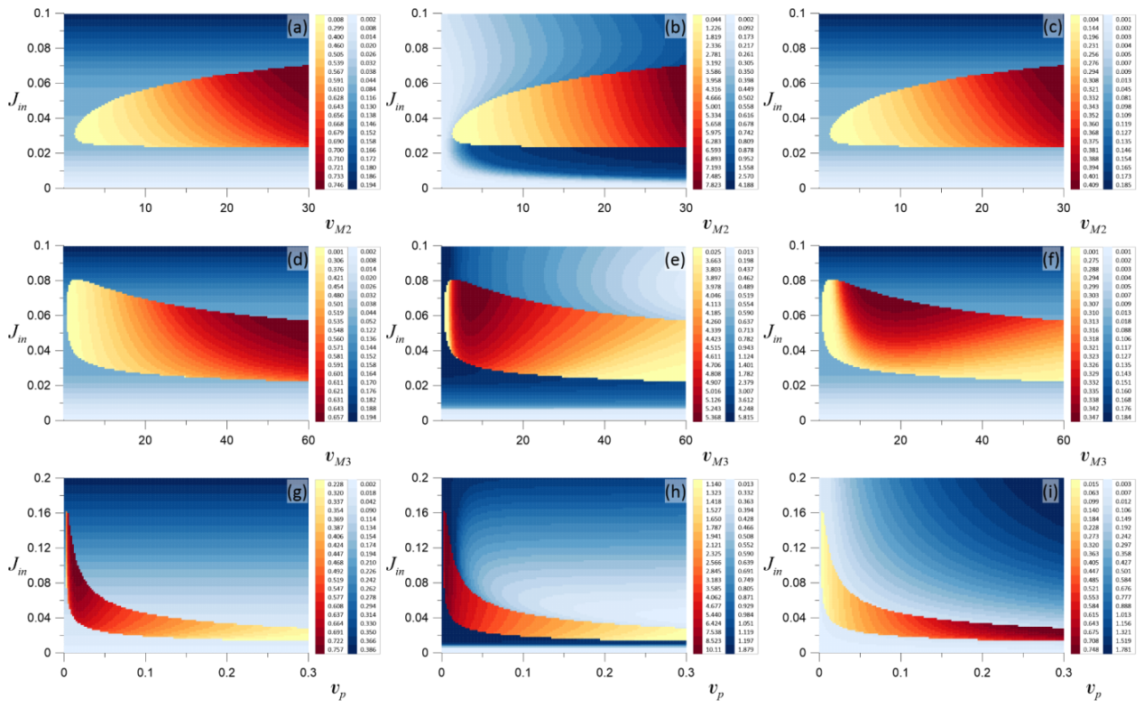
Figure 4.
(a) Two-parametric diagram obtained for and various values of and parameters. As in Figure 3a, the intensity of the blue demonstrates the change of in the equilibrium. The difference between the minimal and the maximal value of in the oscillatory regime is shown by the red-to-yellow gradient. For M/s, the coexisting regimes observed near the upper boundary of the oscillations-to-quiescence transition are shown in (b,c), near the lower boundary—in (d,e). In (g), the difference between the minimal and the maximal value of is shown by a blue curve, and the difference between the minimal and maximal value of is shown by a dashed green curve. In (f,h), the widths of the bistable ranges are presented for lower and upper boundaries, respectively. The blue curve shows the data obtained with the increase of , while the dashed orange curve was calculated with the decrease of .
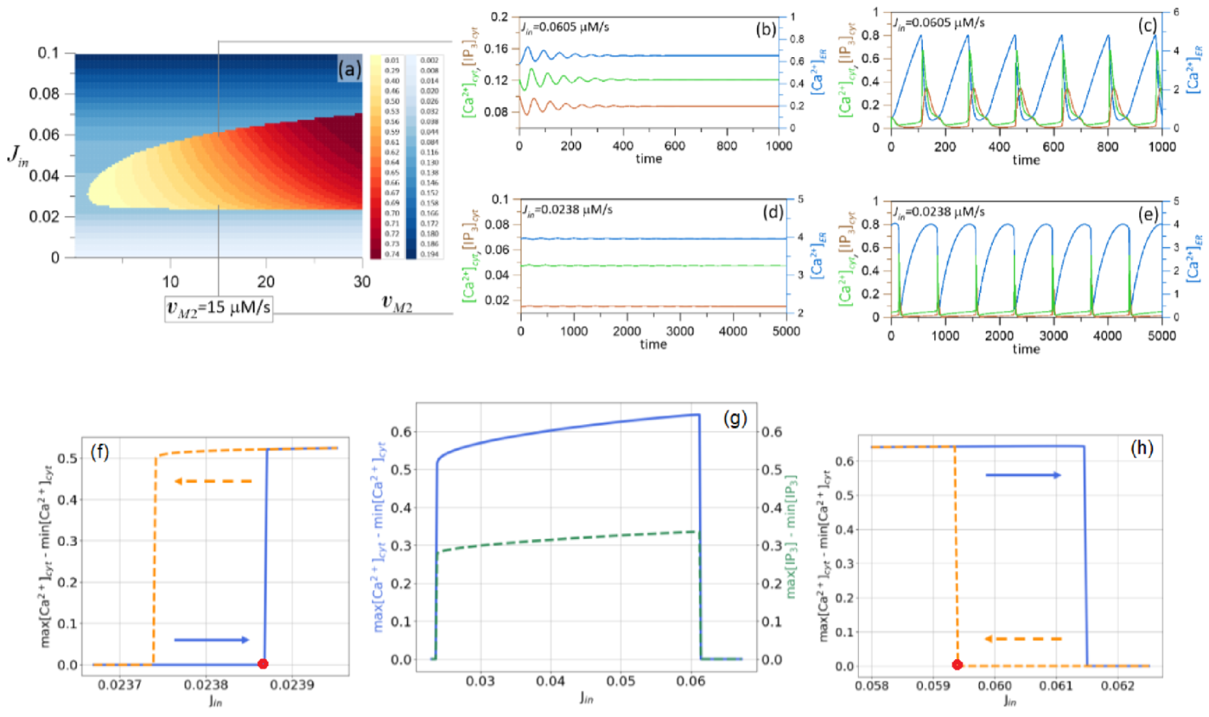
Figure 5.
Two-parametric diagrams obtained for (a,d,g); (b,e,h); and (c,f,i); and for (a–c)—() parameter space; (d–f)—(); and (g–i)—() parameter space. Domains shown in blue correspond to a steady state solution. The intensity of the color demonstrates the change of the corresponding variable in equilibrium. The difference between the minimal and the maximal value of the corresponding variable in the oscillatory regime is shown by a red-to-yellow gradient.
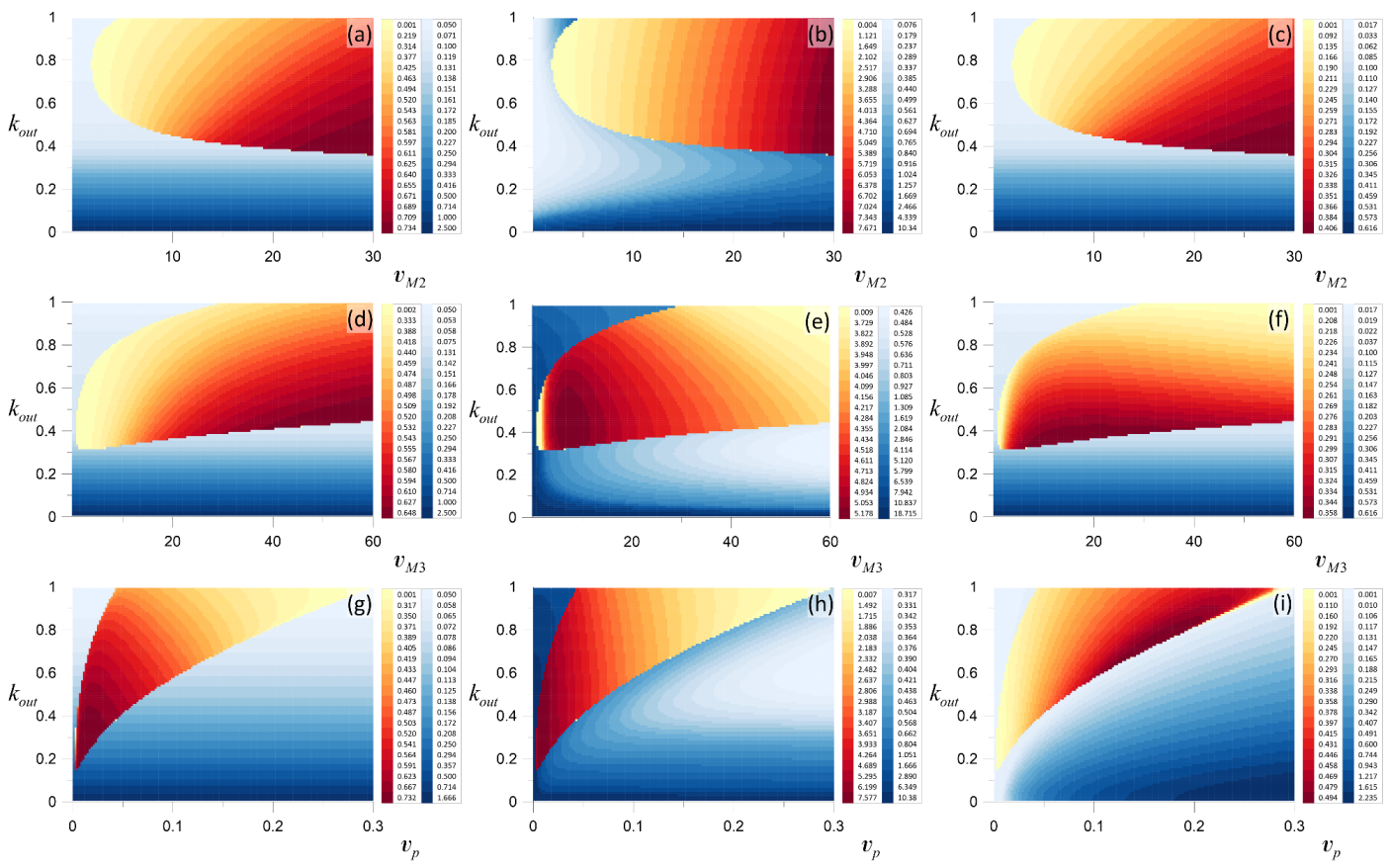
Figure 6.
(a) Time series of ; and (b) corresponding phase portraits obtained for M/s, M/s, , M/s, M, M, M, M, , , ; (c) One-parametric bifurcation diagram shows the local maxima of obtained for various values of the parameter within the time interval [10,000, 15,000]; for each value of , the initial conditions are ; (d) Enlargement of the squared part of the one-parametric bifurcation diagram given in (c); (e) The maximal Lyapunov exponent as function of the parameter .
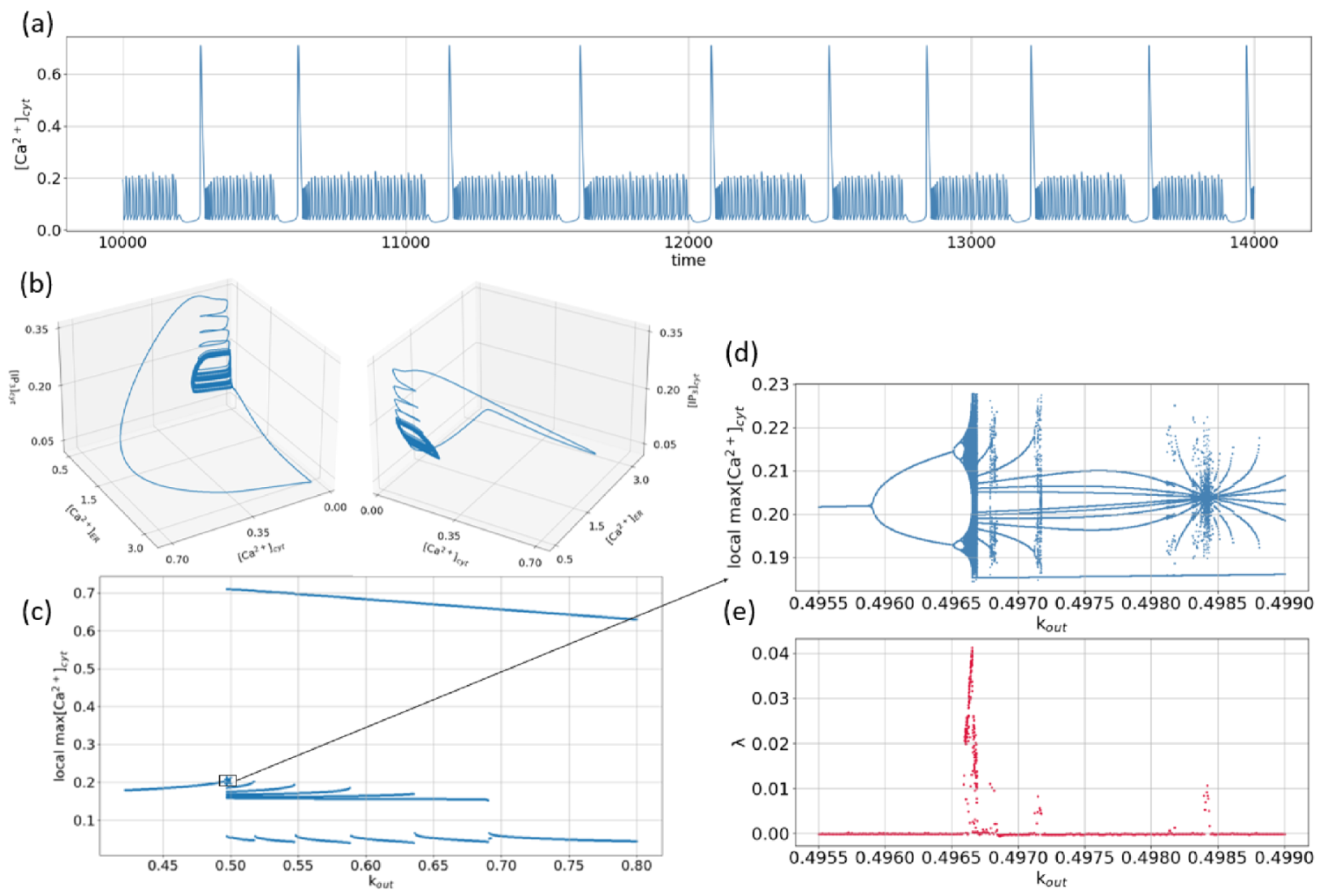
Figure 7.
(a) Time series of ; and (b) corresponding phase portraits obtained for M/s, M/s, , M/s, M, M, M, M, , , ; (c) One-parametric bifurcation diagram shows the local maxima of obtained for various values of the parameter within the time interval [10,000, 15,000]; for each value of , the initial conditions are ; (d) Enlargement of the squared part of the one-parametric bifurcation diagram given in (c); (e) The maximal Lyapunov exponent as function of the parameter .

Figure 8.
(a) Time series of ; and (b) corresponding phase portraits obtained for M/s, M/s, , M/s, M, M, M, M, , , ; (c) One-parametric bifurcation diagram shows the local maxima of obtained for various values of the parameter within the time interval [10,000, 15,000]; for each value of , the initial conditions are ; (d) Enlargement of the squared part of the one-parametric bifurcation diagram given in (c); (e) The maximal Lyapunov exponent as function of the parameter .
Publisher’s Note: MDPI stays neutral with regard to jurisdictional claims in published maps and institutional affiliations. |
© 2022 by the authors. Licensee MDPI, Basel, Switzerland. This article is an open access article distributed under the terms and conditions of the Creative Commons Attribution (CC BY) license (https://creativecommons.org/licenses/by/4.0/).
Share and Cite
MDPI and ACS Style
Pankratova, E.V.; Sinitsina, M.S.; Gordleeva, S.; Kazantsev, V.B. Bistability and Chaos Emergence in Spontaneous Dynamics of Astrocytic Calcium Concentration. Mathematics 2022, 10, 1337. https://doi.org/10.3390/math10081337
AMA Style
Pankratova EV, Sinitsina MS, Gordleeva S, Kazantsev VB. Bistability and Chaos Emergence in Spontaneous Dynamics of Astrocytic Calcium Concentration. Mathematics. 2022; 10(8):1337. https://doi.org/10.3390/math10081337
Chicago/Turabian StylePankratova, Evgeniya V., Maria S. Sinitsina, Susanna Gordleeva, and Victor B. Kazantsev. 2022. "Bistability and Chaos Emergence in Spontaneous Dynamics of Astrocytic Calcium Concentration" Mathematics 10, no. 8: 1337. https://doi.org/10.3390/math10081337
Note that from the first issue of 2016, this journal uses article numbers instead of page numbers. See further details here.