The Case of Small Prime Numbers Versus the Joye–Libert Cryptosystem

Abstract

In this paper, we study the effect of using small prime numbers within the Joye–Libert public key encryption scheme. We introduce two novel versions and prove their security. We further show how to choose the system’s parameters such that the security results hold. Moreover, we provide a practical comparison between the cryptographic algorithms we introduced and the original Joye–Libert cryptosystem.

1. Introduction

The Joye–Libert cryptosystem was introduced in [1,2] as a generalisation of the Goldwasser–Micali public key encryption scheme [3,4]. The main advantage of the Joye–Libert scheme compared to Goldwasser–Micali is that the first supports a larger message space, and thus it considerably decreases the expansion of the ciphertext. Regarding security, the authors prove that inverting the encryption function is equivalent to breaking the quadratic residuosity problem modulo $n=pq$, where p and q are prime numbers. Another important security result is that the scheme is semantically secure if the gap $2^k$-residue assumption modulo n holds. We underline that the Joye–Libert cryptosystem is partially homomorphic with respect to message addition and supports ciphertext randomization.

In this paper, we aim to find a way to improve decryption times for the Joye–Libert scheme. Therefore, we introduce two variants of the system: an unbalanced version and a multiprime one. In the first version, we show how to decrease the size of p, while keeping the system secure and implicitly decreasing the complexity of decryption. The only cryptosystem related to this version is called the unbalanced RSA [5]. Just like our version, the scope is to reduce p, while keeping the system secure.

In the multiprime version, we increase the number of factors while keeping the size of the modulus constant, and we manage to prove that inverting encryption is equivalent to a vectorial form of the quadratic residuosity assumption. We can find only one related cryptosystem in the literature: the multiprime RSA [6,7]. The philosophy behind the multiprime RSA is the same as ours—it uses parallelism to speed up decryption. A bonus of the multiprime Joye–Libert is that we can also use multiple threads to improve encryption time, while in the case of RSA this is not possible.

In the final section of our paper, we analyze the complexity of the two novel variants. Then we compare the decryption time complexities for all versions of the Joye–Libert scheme. If parallelization is possible, then the multiprime variant is to be preferred since it has faster encryption and decryption. Otherwise, the unbalanced version should be used.

Previous work. Note that a preliminary version of this proposal was presented in [8].

Structure of the paper. In Section 2, we provide the notations used in our paper. Then, we recall several definitions needed to describe our proposals. The original Joye–Libert scheme is detailed in Section 3. In Section 4 and Section 5, we present two novel versions of the Joye–Libert scheme. A performance analysis of the Joye–Libert variants is provided in Section 6. Conclusions and open problems are given in Section 7.

2. Preliminaries

Notations. In this paper, $\lambda$ represents a security parameter. By $\left|n\right|$, we denote the size of n in bits. The action of selecting a random element x from a sample space X is denoted by $x\stackrel{\$}{\leftarrow }X$. The assignment operator $x\leftarrow y$ initialises variable x with value y. Let E be an event, then $Pr\left[E\right]$ represents the likelihood of E occurring. Probabilistic polynomial-time algorithms are referred to as PPT algorithms. In this paper, the set of natural numbers $\{0,\dots ,a-1\}$ is denoted by $[0,a)$. To simplify notations, we denote the set $[0,a+1)$ by $[0,a]$. Multidimensional vectors $v=(v_0,\dots ,v_{s-1})$ are represented as $v={\left\{v_i\right\}}_{i\in [0,s)}$.

2.1. Computational Complexity

In this subsection, we present the reader with computational complexities of multiplication, exponentiation and modular inverse. These complexities are needed in order to determine the efficiency of our proposed schemes. Note that the asymptotic values are given in

Table 1. Computational complexity for $\mu$-bit numbers.

Operation	Complexity
Multiplication	$M\left(\mu \right)=\mathcal{O}(\mu log\mu loglog\mu )$
Exponentiation	$\mathcal{O}\left(kM\right(\mu \left)\right)$
Modular inverse	$\mathcal{O}\left(\mu M\right(\mu \left)\right)$

and are taken from [9,10]. To simplify our presentation, we use the notation $M(·)$ for the complexity of the multiplication algorithm. Note that while discussing the complexity of performing an exponentiation, we assume that the exponent’s length is k bits.

2.2. Number Theoretic Prerequisites

The Joye–Libert encryption scheme is based on a generalisation of the Legendre symbol, namely the $2^k$-th power residue symbol. Note that the Legendre symbol is obtained when $k=1$, and for simplicity, we further denote it by ${\displaystyle J_p\left(a\right)}$. We recall the definition of the $2^k$-th power residue symbol and some of its properties, as stated in [11].

Definition 1.

Let p be an odd prime such that $2^k|p-1$. Then, the symbol

$$\begin{array}{c}\hfill {\displaystyle J_{p,2^k}\left(a\right)=a^{\frac{p-1}{2^k}}modp}\end{array}$$

is called the $2^k$-th power residue symbol modulo p, where $a^{\frac{p-1}{2^k}}\in {\mathcal{Z}}_p$, where ${\mathcal{Z}}_p=\{-(p-1)/2,\dots ,-1,0,1,\dots ,(p-1)/2\}$.

Lemma 1.

The $2^k$-th power residue symbol satisfies the following properties

• If $a\equiv bmodp$, then ${\displaystyle J_{p,2^k}\left(a\right)=J_{p,2^k}\left(b\right)}$;
• ${\displaystyle J_{p,2^k}(a^{2^k})=1}$;
• ${\displaystyle J_{p,2^k}\left(ab\right)=J_{p,2^k}\left(a\right)J_{p,2^k}\left(b\right)modp}$;
• ${\displaystyle J_{p,2^k}\left(1\right)=1}$ and ${\displaystyle J_{p,2^k}\left(-1\right)={(-1)}^{(p-1)/2^k}}$.

Let $n=p_1\dots p_t$. We further denote by ${\displaystyle J_n\left(a\right)=J_{p_1}\left(a\right)\dots J_{p_t}\left(a\right)}$ the Jacobi symbol of an integer a modulo an integer n. $J_n$ and $Q{R}_n$ denote the set of integers modulo n with Jacobi symbol 1, and respectively, the set of quadratic residues modulo n.

2.3. Public Key Encryption

The three PPT algorithms specific to a public key encryption (PKE) scheme are: Setup, Encrypt and Decrypt. Given as input a security parameter, the Setup algorithm outputs the public key and the corresponding secret key. To encrypt a message, Encrypt also needs the public key as input in order to output the correlated ciphertext. To recover the original message, the Decrypt algorithm takes as input the secret key and the ciphertext. Note that if decryption fails, Decrypt returns an invalidity symbol.

Definition 2

(Indistinguishability under Chosen Plaintext Attacks—ind-cpa) The security model against chosen plaintext attacks for a PKE scheme is described using the following game:

$Setup\left(\lambda \right)$: In this phase, challenger C first computes the public key, while keeping the corresponding secret key to himself. Then C sends only the public key to adversary A.

$Query$: Adversary A chooses two equal length messages $m_0,m_1$ and sends them to C. After flipping a coin $b\in \{0,1\}$, the challenger encrypts $m_b$ and sends to A the resulting ciphertext.

$Guess$: In this phase, the adversary outputs a guess $b^{\prime }\in \{0,1\}$. A wins the security game if $b^{\prime }=b$.

The advantage of an adversary A attacking a PKE scheme is defined as

$$\begin{array}{c}\hfill {ADV}_A^{\mathrm{IND}-\mathrm{CPA}}\left(\lambda \right)=|Pr[b=b^{\prime }]-1/2|\end{array}$$

where the probability is computed over the random bits used by C and A. A PKE scheme isind-cpasecure if for any PPT adversary A, the advantage ${ADV}_A^{\mathrm{IND}-\mathrm{CPA}}\left(\lambda \right)$ is negligible.

3. The Joye–Libert PKE Scheme

The Joye–Libert encryption scheme was initially introduced in [1]. Its security was improved in [2]. The authors proved that inverting the encryption function is as hard as the quadratic residuosity assumption. Joye et al. also showed that in the standard model, the ind-cpa security of the PKE is equivalent to the gap $2^k$-residuosity assumption. We shortly present the algorithms of the Joye–Libert cryptosystem.

Setup($\lambda$): Set an integer $k\ge 1$. Randomly generate two distinct large prime numbers p, q such that $\left|p\right|=\left|q\right|=\lambda$ and $p\equiv 1mod{2}^k$. Output the public key $pk=(n,y,k)$, where $n=pq$ and $y\in J_n\setminus Q{R}_n$. The corresponding secret key is $sk=(p,q)$.

Encrypt($pk,m$): To encrypt a message $m\in [0,2^k)$, we choose $x\stackrel{\$}{\leftarrow }{\mathbb{Z}}_n^{*}$ and compute $c\equiv y^m{x}^{2^k}modn$. Output the ciphertext c.

Decrypt($sk,c$): Compute the value ${\displaystyle z\equiv J_{p,2^k}\left(c\right)}$ and find m such that the relation ${\left[{\displaystyle J_{p,2^k}\left(y\right)}\right]}^m\equiv zmodp$ holds. Efficient methods to recover m can be found in a subsequent section.

4. The Unbalanced Joye–Libert PKE Scheme

In the unbalanced Joye–Libert scheme, we reduce the size of p (denoted by ${\lambda }_p$) while keeping the size of n constant (denoted by ${\lambda }_n$). This modification only impacts the description of the Setup algorithm, which we briefly describe below. Therefore, we have ${\lambda }_n={\lambda }_p+{\lambda }_q$, where ${\lambda }_q=\left|q\right|$ and ${\lambda }_p\le {\lambda }_q$. Note that when ${\lambda }_p={\lambda }_q$, we obtain the Joye–Libert cryptosystem, which we further refer to as the balanced Joye–Libert scheme.

Setup(${\lambda }_p,{\lambda }_q$): Set an integer $k\ge 1$. Randomly generate two distinct large prime numbers p, q such that $\left|p\right|={\lambda }_p$, $\left|q\right|={\lambda }_q$ and $p\equiv 1mod{2}^k$. Output the public key $pk=(n,y,k)$, where $n=pq$ and $y\in J_n\setminus Q{R}_n$. The corresponding secret key is $sk=(p,q)$.

Remark 1.

Modifying the size of p does not impact the security proofs discussed in [1,2]. Therefore, as long as factoring is hard, the unbalanced version is secure. We show how to choose ${\lambda }_p$ such that factoring remains difficult in Section 6.

5. The Multiprime Joye–Libert PKE Scheme

5.1. Description

We further describe the multiprime Joye–Libert encryption scheme. In this case, we split up n into multiple primes. Therefore, we have ${\lambda }_n=t{\lambda }_p+{\lambda }_q$. Note that when ${\lambda }_p={\lambda }_q$ and $t=1$, we obtain the original cryptosystem from [1,2], and moreover, when in addition we set $k=1$, we obtain the Goldwasser–Micali cryptosystem [3]. In addition, if we set $t=1$, we obtain the unbalanced version.

Setup(${\lambda }_p,{\lambda }_q$): Set an integer $k\ge 1$. Randomly generate $t+1$ distinct large prime numbers $p_1,\dots ,p_t,q$ such that $|p_1|=\dots =|p_t|={\lambda }_p$, $\left|q\right|={\lambda }_q$ and $p_1,\dots ,p_t\equiv 1mod{2}^k$. Let $n=p_1\dots p_{t}q$. For each $i\in [1,t]$ select $y_i\stackrel{\$}{\leftarrow }{\mathbb{Z}}_n^{*}$ such that

$$\begin{array}{c}\hfill {\displaystyle J_{p_i}\left(y_i\right)=J_q\left(y_i\right)=-1\mathrm{and}{J}_{p_j,2^k}\left(y_i\right)=1,\mathrm{where}j\ne i.}\end{array}$$

Output the public key $pk=(n,Y,k)$ and the corresponding secret key $sk=P$, where $Y={\left\{y_i\right\}}_{i\in [1,t]}$ and $P={\left\{p_i\right\}}_{i\in [1,t]}$.

Encrypt($pk,m$): To encrypt message $m\in [0,2^{k}t)$, first we divide it into t blocks $m=m_1\parallel \dots \parallel m_t$ such that for each $i\in [1,t]$ we have $|m_i|=k$. Then, we choose randomly $x\stackrel{\$}{\leftarrow }{\mathbb{Z}}_n^{*}$ and compute the value $c\equiv x^{2^k}·{\prod }_{i=1}^t{y}_i^{m_i}modn$. The output is ciphertext c.

Decrypt($sk,c$): For each $i\in [1,t]$, compute $m_i$ using Algorithm 1.

Algorithm 1 Basic decryption algorithm

Correctness. Let $m_i={\sum }_{w=0}^{k-1}{b}_w{2}^w$ be the binary expansion of block $m_i$. Note that

$$\begin{array}{c}\hfill {\displaystyle J_{p_i,2^s}\left(c\right)=J_{p_i,2^s}(x^{2^k}·\prod _{v=1}^t{y}_v^{m_v})=J_{p_i,2^s}\left(y_i^{m_i}\right)=J_{p_i,2^s}{\left(y_i\right)}^{{\sum }_{w=0}^{s-1}{b}_w{2}^w}}\end{array}$$

since

• ${\displaystyle J_{p_i,2^s}(x^{2^k})=1}$, where $1\le s\le k$;
• ${\displaystyle J_{p_i,2^k}(y_j)=1}$, where $j\ne i$;
• ${\sum }_{w=0}^{k-1}{b}_w{2}^w=\left({\sum }_{w=0}^{s-1}{b}_w{2}^w\right)+2^s\left({\sum }_{w=s}^{k-1}{b}_w{2}^{w-s}\right)$.

As a result, the message block $m_i$ can be recovered bit-by-bit using $p_i$.

5.2. Security Analysis

In this section, we first introduce a vectorial generalisation of the quadratic residuosity problem and prove that inverting the encryption function of our proposal is as hard as breaking this assumption. Then, we generalise the gap $2^k$-residuosity problem stated in [1] and prove the ind-cpa security of our proposal.

Before stating the security assumptions used to prove the security of our proposal, we first define the following sets

$$\begin{array}{cc}\hfill {\mathbb{Z}}_n\left(i\right)& {\displaystyle =\{x\in {\mathbb{Z}}_n^{*}\mid J_{p_j,2^k}\left(x\right)=1\mathrm{for}\mathrm{any}j\ne i\},}\hfill \\ \hfill Q{R}_n\left(i\right)& {\displaystyle =\{x\in {\mathbb{Z}}_n\left(i\right)\mid J_{p_i}\left(x\right)=1\mathrm{and}{J}_q\left(x\right)=1\},}\hfill \\ \hfill J_n\left(i\right)& {\displaystyle =\{x\in {\mathbb{Z}}_n\left(i\right)\mid J_{p_i}\left(x\right)J_q\left(x\right)=1\},}\hfill \end{array}$$

where $n=p_1\dots p_{t}q$ and $i,j\in [1,t]$.

Definition 3

Vectorial Quadratic Residuosity—vqr). Choose $t+1$ distinct large prime numbers $p_1,\dots ,p_t,q$ such that $|p_1|=\dots =|p_t|={\lambda }_p$, $\left|q\right|={\lambda }_q$ and $p_1,\dots ,p_t\equiv 1mod{2}^k$. Let $n=p_1\dots p_{t}q$. Let A be a PPT algorithm that returns 1 on input $(x_1,\dots ,x_t,n)$ if $x_i\in Q{R}_n\left(i\right)$. We define the advantage

$$\begin{array}{cc}\hfill {ADV}_A^{\mathrm{VQR}}({\lambda }_p,{\lambda }_q)& =\left|Pr[A(x_1,\dots ,x_t,n)=1|x_i\stackrel{\$}{\leftarrow }Q{R}_n\left(i\right)\mathrm{for}i\in [1,t]]\right.\hfill \\ & \left.-Pr[A(x_1,\dots ,x_t,n)=1|x_i\stackrel{\$}{\leftarrow }{J}_n\left(i\right)\setminus Q{R}_n\left(i\right)\mathrm{for}i\in [1,t]]\right|.\hfill \end{array}$$

The Vectorial Quadratic Residuosity assumption states that for any PPT algorithm A the advantage ${ADV}_A^{\mathrm{VQR}}({\lambda }_p,{\lambda }_q)$ is negligible.

Theorem 1.

Inverting the encryption function of the multiprime Joye–Libert PKE is intractable if thevqrassumption is intractable.

Proof. 

Let us assume that there exists an adversary A such that given a ciphertext c, it recovers the message m. We construct a PPT algorithm that breaks the vqr assumption. More precisely, on input $(y_1,\dots ,y_t)$B computes $c\equiv {(y_1\dots y_t)}^{2^{k-1}}{x}^{2^k}$, where $x\stackrel{\$}{\leftarrow }{\mathbb{Z}}_n^{*}$. Remark that if $y_i\in J_n\left(i\right)\setminus Q{R}_n\left(i\right)$, then c is an encryption of $m_{2^{k-1}}=2^{k-1}\parallel \dots \parallel 2^{k-1}$. If $y_i\in Q{R}_n\left(i\right)$, then $y_i\equiv w_i^{2}modn$, and thus $c\equiv {(w_1\dots w_{t}x)}^{2^k}modn$ is an encryption of $m_0=0$. According to the above arguments, on input $(y_1,\dots ,y_t,c)$ algorithm A outputs either $m_{2^{k-1}}$ or $m_0$, and thus B outputs 0 or 1, respectively. Therefore, B breaks the vqr assumption with non-negligible probability.    □

Definition 4

(Vectorial Gap $2^k$-Residuosity—vgr). Choose $t+1$ distinct large prime numbers $p_1,\dots ,p_t,q$ such that $|p_1|=\dots =|p_t|={\lambda }_p$, $\left|q\right|={\lambda }_q$ and $p_1,\dots ,p_t\equiv 1mod{2}^k$. Let $n=p_1\dots p_{t}q$. Let A be a PPT algorithm that returns 1 on input $(x_1,\dots ,x_t,k,n)$ if $x_i\in J_n\left(i\right)\setminus Q{R}_n\left(i\right)$. We define the advantage

$$\begin{array}{cc}\hfill {ADV}_A^{\mathrm{VGR}}({\lambda }_p,{\lambda }_q)& =\left|Pr[A(x_1,\dots ,x_t,k,n)=1|x_i\stackrel{\$}{\leftarrow }{J}_n\left(i\right)\setminus Q{R}_n\left(i\right)\mathrm{for}i\in [1,t]]\right.\hfill \\ & \left.-Pr[A(x_1^{2^k},\dots ,x_t^{2^k},k,n)=1|x_i\stackrel{\$}{\leftarrow }{\mathbb{Z}}_n^{*}\mathrm{for}i\in [1,t]]\right|.\hfill \end{array}$$

The Vectorial Gap $2^k$-Residuosity assumption states that for any PPT algorithm A, the advantage ${ADV}_A^{\mathrm{VGR}}({\lambda }_p,{\lambda }_q)$ is negligible.

Theorem 2.

The multiprime Joye–Libert PKE isind-cpasecure if and only if thevgrassumption is intractable.

Proof. 

The proof of the statement is obtained by simply replacing the distribution of the public key elements $(y_1,\dots ,y_t)$. More precisely, we randomly select the $y_i$ values from the multiplicative subgroup of $2^k$ residues modulo n instead of drawing them from the $J_n\left(i\right)\setminus Q{R}_n\left(i\right)$ set. Under the vgr assumption, the adversary will not notice this change. Therefore, we removed any link between the ciphertext c and the message m, and thus the ind-cpa security follows.    □

5.3. Optimizations

Setup Optimization. When choosing the public key we have to meet certain restrictions. An effective way to accomplish this is to first randomly choose the values $y_{i,i}\stackrel{\$}{\leftarrow }{\mathbb{Z}}_{p_i}^{*}\setminus Q{R}_{p_i}$, $y_{i,t+1}\stackrel{\$}{\leftarrow }{\mathbb{Z}}_q^{*}\setminus Q{R}_q$ and $w_{i,j}\stackrel{\$}{\leftarrow }{\mathbb{Z}}_{p_j}^{*}$. Then compute the elements $y_{i,j}\leftarrow w_{i,j}^{2^k}mod{p}_j$. Using the Chinese remainder theorem, we compute the desired value $y_i\in {\mathbb{Z}}_n^{*}$ such that $y_i\equiv y_{i,\ell }mod{p}_{\ell }$ for all $\ell \in [1,t]$ and $y_i\equiv y_{i,t+1}modq$.

Decryption Optimization. In order to speed-up the decryption process, the authors of [2] add an extra restriction when generating the prime factors of n, and then use it to simplify decryption. Applying this to the multiprime case, we obtain the fact that we have to generate $p_i$ such that $p_i\not\equiv 1mod{2}^{k+1}$ holds.

Let $p_i^{\prime }=(p_i-1)/2^k$ and ${\alpha }_i\left[s\right]=2^{k-s}{p}_i^{\prime }$. Then, the following relation between the ciphertext and plaintext holds

$$\begin{array}{cc}\hfill c^{{\alpha }_i\left[s\right]}& \equiv {(x^{2^k}·\prod _{v=1}^t{y}_v^{m_v})}^{{\alpha }_i\left[s\right]}\hfill \\ \hfill & \equiv y_i^{{\alpha }_i\left[s\right]{\sum }_{w=0}^{s-1}{b}_w{2}^w}\hfill \\ \hfill & \equiv y_i^{b_{s-1}{2}^{k-1}{p}_i^{\prime }}{y}_i^{{\alpha }_i\left[s\right]{\sum }_{w=0}^{s-2}{b}_w{2}^w}\hfill \\ \hfill & \equiv {(-1)}^{b_{s-1}}{y}_i^{{\alpha }_i\left[s\right](m_{i}mod{2}^{s-1})}mod{p}_i\hfill \end{array}$$

since

• ${(x^{2^k})}^{{\alpha }_i\left[s\right]}=x^{2^{k-s}(p_i-1)}=1$;
• ${\displaystyle J_{p_i,2^k}\left(y_j\right)=1}$, where $j\ne i$;
• ${\sum }_{w=0}^{k-1}{b}_w{2}^w=\left({\sum }_{w=0}^{s-1}{b}_w{2}^w\right)+2^s\left({\sum }_{w=s}^{k-1}{b}_w{2}^{w-s}\right)$;
• ${\displaystyle J_{p_i}\left(y_i\right)=-1}$.

Hence, if we precompute $D_i=y_i^{-p_i^{\prime }}$, then we can recover message block $m_i$. Wrapping it all together, we obtain Algorithm 2. Note that when $t=1$, we obtain [2] (Algorithm 3). The authors also propose three other optimizations [2] (Algorithms 4–6), but their complexity is similar to that of Algorithm 3. Remark that two of these optimizations contain a typo: in line 5, Algorithm 5 and line 6, Algorithm 6 we should have $A^{k-j}\ne C[k-j]modp$ instead of $A\ne C[k-j]modp$.   

Algorithm 2 Optimized decryption algorithm

6. Implementation and Performance Analysis

6.1. Parameter Selection

The fastest currently known algorithm for factoring composite numbers is the Number Field Sieve (NFS) [12]. The expected running time of the NFS depends on the size of the modulus n and not on the size of its factors. More precisely, the expected running time is approximately

$$\begin{array}{c}\hfill L\left[n\right]=e^{1.923{(logn)}^{1/3}{(loglogn)}^{2/3}}.\end{array}$$

In [12,13], the authors extrapolate the running time needed to factor a modulus of size ${\lambda }_n$ from the computational effort required to factor a 512-bit modulus. Hence, a ${\lambda }_n$-bit modulus offers a security equivalent to a block cipher of d-bit security if

$$\begin{array}{c}\hfill L\left[2^{{\lambda }_n}\right]\simeq 50·2^{d-56}·L\left[2^{512}\right].\end{array}$$

(1)

Since we start from a secure Joye–Libert PKE and we wish to optimize decryption by decreasing the size of some of the factors of the modulus, while keeping the size of the modulus constant, the NFS cannot be expected to factor n. Unfortunately, this strategy can make the resulting PKEs vulnerable to the Elliptic Curve Method (ECM) [14] if we lower the size of the factors below a certain threshold. Compared to the NFS, the ECM has a running time determined by the size of the smallest factor. Thus, if p is the smallest factor, then the running time of the ECM is

$$\begin{array}{c}\hfill E[n,p]={\left({log}_{2}n\right)}^2{e}^{\sqrt{2logploglogp}}.\end{array}$$

Similarly to the NFS, Lenstra [15] extrapolates the equivalent security provided by a module of size ${\lambda }_n$ with the smallest prime of size ${\lambda }_p$ to be

$$\begin{array}{c}\hfill E[2^{{\lambda }_n},2^{{\lambda }_p}]\ge 80·2^{d-56}·E[2^{768},2^{167}].\end{array}$$

(2)

From Equations (1) and (2), we can deduce the following equivalency

$$\begin{array}{c}\hfill E[2^{{\lambda }_n},2^{{\lambda }_p}]\ge 80·2^{{log}_2(L\left[2^{{\lambda }_n}\right]/(50·L\left[2^{512}\right]))}·E[2^{768},2^{167}].\end{array}$$

(3)

A different model for predicting the security against the NFS and the ECM is provided in [16]. Compared to Lenstra’s model, Brent uses known historical factoring records to predict the year a modulus of a given size will be factored. Using the least-squares fit, Brent obtains the following equation for the NFS

$$\begin{array}{c}\hfill D_n^{1/3}=\frac{Y-1928.6}{13.24}\mathrm{or}\mathrm{equivalently}Y=13.24·D_n^{1/3}+1928.6\end{array}$$

(4)

and for the ECM

$$\begin{array}{c}\hfill D_p^{1/2}=\frac{Y-1932.3}{9.3}\mathrm{or}\mathrm{equivalently}Y=9.3·D_p^{1/2}+1932.3,\end{array}$$

(5)

where $D_n$ is the number of digits of the factored modulus and $D_p$ is the number of digits of the largest prime factor found using the ECM.

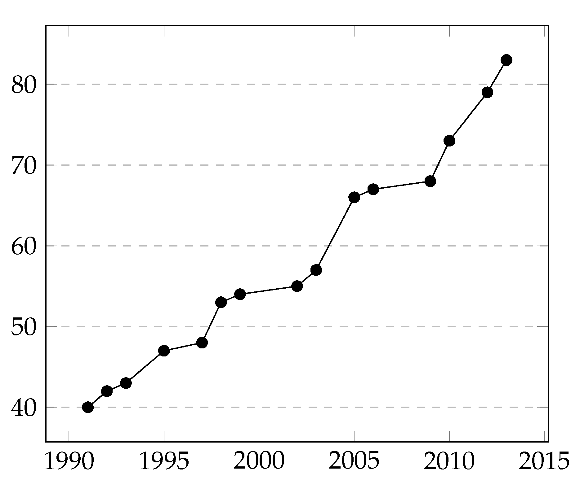
Using regression analysis, we update Brent’s equations using data points from [17,18,19,20,21,22,23,24,25,26,27] for the NFS and from [28,29] for the ECM. These data points are presented in Figure 1 and Figure 2.

Therefore, the updated equation for the NFS is

$$\begin{array}{c}\hfill D_n^{1/3}=\frac{Y-1926}{13.97}\mathrm{or}\mathrm{equivalently}Y=13.97·D_n^{1/3}+1926\end{array}$$

(6)

and for the ECM

$$\begin{array}{c}\hfill D_p^{1/2}=\frac{Y-1939}{8.207}\mathrm{or}\mathrm{equivalently}Y=8.207·D_p^{1/2}+1939.\end{array}$$

(7)

Equations (4)–(7) are presented in Figure 3 and Figure 4. Note that the black dots represent the acquired data points. We observe that in the case of the NFS the estimates are close, while in the case of the ECM the new estimate is more pessimistic from a security point of view. Using the updated estimates (Equations (6) and (7)), we obtain the following equivalency

$$\begin{array}{c}\hfill D_p^{1/2}=\frac{13.97·D_n^{1/3}-13}{8.207}.\end{array}$$

(8)

According to NIST [30], the recommended key sizes for composite modules are ${\lambda }_n=1536/3840/15,360$. We preferred to use NIST recommendations instead of the ones from [12,13], since these key sizes are the ones used by the industry and the key sizes from [12,13] are criticized as being too conservative [17]. Therefore, using Equations (3) and (8), we obtain the equivalent size of the smallest prime. The results are presented in

Table 2. Equivalent key sizes.

Modulus Key Size	3072	7680	15,360
Lenstra model	$800\left(3\right)$	$1617\left(4\right)$	$2761\left(5\right)$
Regression model	$749\left(4\right)$	$1457\left(5\right)$	$2385\left(6\right)$

. Note that in the parentheses we provide the maximum number of prime factors that n can have. Based on these equivalences, we obtain the parameters for the Joye–Libert schemes that offer protection against the NFS and the ECM (see

Table 3. Joye–Libert parameters’ size.r.

$\left|\mathit{n}\right|$	t	$\left|\mathit{p}\right|$	$\left|\mathit{q}\right|$	$|{\mathit{m}}_{\mathit{i}}|$	Type	Model
3072	1	1536	1536	128	Balanced	-
	1	800	2272	128	Unbalanced	Lenstra
	2	800	1472	64	Multiprime
	1	749	2323	128	Unbalanced	Regression
	2	749	1574	64	Multiprime
	3	749	825	43
7680	1	3840	3840	192	Balanced	-
	1	1617	6063	192	Unbalanced	Lenstra
	2	1617	4446	96	Multiprime
	3	1617	2829	64
	1	1457	6223	192	Unbalanced	Regression
	2	1457	4766	96	Multiprime
	3	1457	3309	64
	4	1457	1852	48
15,360	1	7680	7680	256	Balanced	-
	1	2761	12,599	256	Unbalanced	Lenstra
	2	2761	9838	128	Multiprime
	3	2761	7077	86
	4	2761	4316	64
	1	2385	12,975	256	Unbalanced	Regression
	2	2385	10,590	128	Multiprime
	3	2385	8205	86
	4	2385	5820	64
	5	2385	3435	52

).

Due to a powerful attack by Coppersmith [31], the size of k must be upper bounded by $0.5{\lambda }_p$. Otherwise, the factors of n can be found. We can easily see that the block sizes from Table 3 offer a large enough security margin obtained from this bound (see

Table 4. Coppersmith’s upper bound.

$\left|p\right|$	1536	800	749	3840	1617	1457	7680	2761	2385
$0.5\left|p\right|$	768	400	374	1920	808	728	3840	1380	1192

).

6.2. Complexity

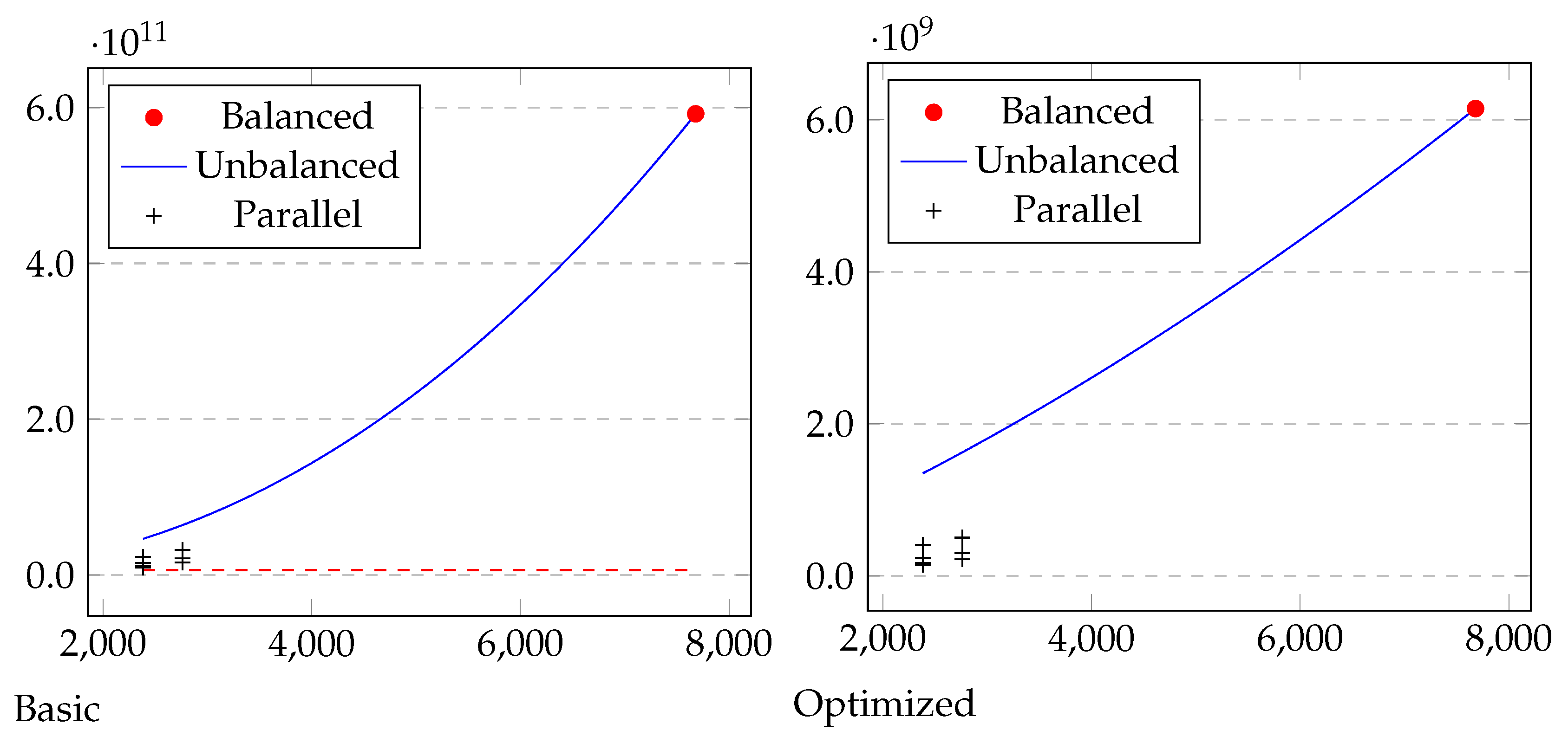
Using the complexities provided in Table 1, we compute the asymptotic run times of the decryption algorithm for each Joye–Libert variant. We also determine the size of a block $m_i$ for each variant. The results are provided in

Table 5. Performance analysis.

Scheme	$\left|\mathit{m}\right|$	Encryption Complexity	Decryption Complexity
Balanced	k	$\mathcal{O}\left(2kM\left({\lambda }_n\right)\right)$	$\mathcal{O}\left(\right(2k\lambda +k\left)M\right(\lambda \left)\right)$
			$\mathcal{O}\left((\lambda +k^2/2+3k/2)M\left(\lambda \right)\right)$
Unbalanced	k	$\mathcal{O}\left(2kM\left({\lambda }_n\right)\right)$	$\mathcal{O}\left((2k{\lambda }_p+k)M\left({\lambda }_p\right)\right)$
			$\mathcal{O}\left(({\lambda }_p+k^2/2+3k/2)M\left({\lambda }_p\right)\right)$
Multiprime	$tk$	$\mathcal{O}\left(2ktM\left({\lambda }_n\right)\right)$	$\mathcal{O}\left(t(2k{\lambda }_p+k)M\left({\lambda }_p\right)\right)$
			$\mathcal{O}\left(t({\lambda }_p+k^2/2+3k/2)M\left({\lambda }_p\right)\right)$
Parallel Multiprime	$tk$	$\mathcal{O}\left(2kM\left({\lambda }_n\right)\right)$	$\mathcal{O}\left((2k{\lambda }_p+k)M\left({\lambda }_p\right)\right)$
			$\mathcal{O}\left(({\lambda }_p+k^2/2+3k/2)M\left({\lambda }_p\right)\right)$

. Note that by parallel multiprime we mean the multiprime version in which we use a separate thread to compute each block $m_i$. We can easily see that for the parameters presented in Table 3, the encryption and decryption complexities of the unbalanced and multiprime versions are similar. Therefore, we only compare the balanced, unbalanced and the parallel multiprime versions. In addition, remark that we choose the parameters such that the message spaces are similar for all the variants.

The comparison of the computational complexity of the three variants is presented in Figure 5, Figure 6 and Figure 7. Note that the two sets of crosses for the multiprime version correspond to the two equivalence models: Lenstra—right side crosses and Regression—left side crosses. We also added a dotted red line in the case of the basic decryption (Algorithm 1), which represents the boundary of the optimized decryption algorithm (Algorithm 2) of the balanced version.

From the six plots, we can see that the parallel multiprime version always performs better than the (un)balanced version if multiple threads are available. Additionally, the more threads we use, the faster we recover the original message. Therefore, if additional memory is available and parallelization is possible, then the parallel multiprime version endowed with the optimized decryption algorithm is preferable. Nevertheless, if we only have access to parallelization, then the parallel multiprime version equipped with the basic decryption algorithm is the best choice. Otherwise, we should use the unbalanced variant.

6.3. Implementation Details

We further provide the reader with benchmarks for the three Joye–Libert PKE schemes. We ran each of the three sub-algorithms on a CPU Intel i7-4790 4.00 GHz and used GCC to compile it (with the O3 flag activated for optimization). Note that for all computations we used the GMP library [32]. To calculate the running times we used the omp_get_wtime() function [33]. For the parallel multiprime variant we used the OMP library [33] to parallelize encryption/decryption. To obtain the average running time in seconds we chose to encrypt 100 $128/192/256$-bit messages. Therefore, we wanted to simulate a key distribution scenario. The results are provided in

Table 6. Running times.

$\left|\mathit{n}\right|$	t	$\left|\mathit{p}\right|$	Setup	Encrypt	Decrypt	Decrypt (opt)
3072	1	1536	$0.193475$	$0.000782$	$0.325478$	$0.007954$
	1	800	$0.414516$	$0.000783$	$0.046704$	$0.002073$
	2	800	$0.129921$	$0.000584$	$0.025147$	$0.001427$
	1	749	$0.507081$	$0.000782$	$0.038254$	$0.001796$
	2	749	$0.140442$	$0.000567$	$0.020635$	$0.001273$
	3	749	$0.036575$	$0.000419$	$0.014810$	$0.000770$
7680	1	3840	$6.554910$	$0.004791$	$6.516350$	$0.095550$
	1	1617	$14.48600$	$0.004792$	$0.565853$	$0.017291$
	2	1617	$6.103730$	$0.003115$	$0.287015$	$0.006300$
	3	1617	$1.334260$	$0.002326$	$0.205834$	$0.004104$
	1	1457	$17.03100$	$0.004790$	$0.390024$	$0.013370$
	2	1457	$6.961240$	$0.003112$	$0.201755$	$0.004917$
	3	1457	$2.030210$	$0.002387$	$0.162581$	$0.003348$
	4	1457	$0.559723$	$0.001948$	$0.154818$	$0.002867$
15,360	1	7680	$55.77040$	$0.018572$	$47.62750$	$0.472317$
	1	2761	$184.5970$	$0.018570$	$3.337000$	$0.080039$
	2	2761	$69.75550$	$0.010459$	$1.712070$	$0.029658$
	3	2761	$27.77600$	$0.007987$	$1.222490$	$0.023583$
	4	2761	$8.610660$	$0.006857$	$0.995357$	$0.018094$
	1	2385	$183.5240$	$0.018564$	$2.183190$	$0.059934$
	2	2385	$86.03020$	$0.010578$	$1.135120$	$0.021922$
	3	2385	$38.94160$	$0.008167$	$0.808199$	$0.017175$
	4	2385	$16.45910$	$0.006833$	$0.675422$	$0.012873$
	5	2385	$5.086330$	$0.006127$	$0.702819$	$0.012128$

. Note that the optimized version of the decryption algorithm is denoted by Decrypt (opt).

We can see from Table 6 that the conclusions presented in Section 6.2 hold. We can also see that the multiprime version has the shortest time to generate the parameters, while the unbalanced version the longest time. Nevertheless, generating parameters is a one-time operation.

7. Conclusions

In this work, we introduced two novel versions of the Joye-Libert cryptosystem. The first one, called the unbalanced Joye–Libert PKE, lowers the size of p in order to decrease decryption time. The second one, called the multiprime Joye–Libert PKE, increases the number of factors and achieves better decryption times by using multiple threads. Therefore, if parallel threads are available, we recommend the multiprime version, otherwise, we recommend the unbalanced variant. If additional memory is available, then we can replace the basic decryption algorithm with the optimized version, and therefore, we can obtain even better decryption times.

Open Problem. In [2], the authors manage to link the gap $2^k$-residuosity assumption to the quadratic residuosity assumption, when $q\equiv 3mod4$, and to the quadratic residuosity and squared Jacobi symbols assumptions, when $q\equiv 1mod4$. Therefore, it would be interesting to find a similar link for the vqr assumption. The main bottleneck that we encountered when trying to link it to the vqr is that the probability of choosing an element from $J_n\left(i\right)$ is $1/2^{kt-k+2}$, and thus for t elements the probability is $1/2^{t(kt-k+2)}$. Therefore, for practical values of k and t, this probability is negligible.

References

- Joye, M.; Libert, B. Efficient Cryptosystems from 2k-th Power Residue Symbols. In Proceedings of the Annual International Conference on the Theory and Applications of Cryptographic Techniques, Athens, Greece, 26–30 May 2013; Lecture Notes in Computer Science. Springer: Berlin/Heidelberg, Germany, 2013; Volume 7881, pp. 76–92. [Google Scholar]
- Benhamouda, F.; Herranz, J.; Joye, M.; Libert, B. Efficient Cryptosystems from 2k-th Power Residue Symbols. J. Cryptol. 2017, 30, 519–549. [Google Scholar] [CrossRef] [Green Version]
- Goldwasser, S.; Micali, S. Probabilistic Encryption and How to Play Mental Poker Keeping Secret All Partial Information; STOC 1982; ACM: New York, NY, USA, 1982; pp. 365–377. [Google Scholar]
- Goldwasser, S.; Micali, S. Probabilistic Encryption. J. Comput. Syst. Sci. 1984, 28, 270–299. [Google Scholar] [CrossRef] [Green Version]
- Shamir, A. RSA for Paranoids. RSA Lab. Cryptobytes 1995, 1, 1–4. [Google Scholar]
- Rivest, R.L.; Shamir, A.; Adleman, L.M. Cryptographic Communications System and Method. US Patent 4,405,829, 20 September 1983. [Google Scholar]
- Cryptography Using Compaq Multiprime Technology in a Parallel Processing Environment. 2000. Available online: https://www.compaq.com (accessed on 24 March 2022).
- Maimuţ, D.; Teşeleanu, G. A New Generalisation of the Goldwasser-Micali Cryptosystem Based on the Gap 2k-residuosity Assumption. In Proceedings of the International Conference on Information Technology and Communications Security, Bucharest, Romania, 19–20 November 2020; Lecture Notes in Computer Science. Springer: Berlin/Heidelberg, Germany, 2020; Volume 12596, pp. 24–40. [Google Scholar]
- Crandall, R.; Pomerance, C. Prime Numbers: A Computational Perspective; Number Theory and Discrete Mathematics; Springer: Berlin/Heidelberg, Germany, 2005. [Google Scholar]
- Menezes, A.; van Oorschot, P.C.; Vanstone, S.A. Handbook of Applied Cryptography; CRC Press: Boca Raton, FL, USA, 1996. [Google Scholar]
- Yan, S.Y. Number Theory for Computing; Theoretical Computer Science; Springer: Berlin/Heidelberg, Germany, 2002. [Google Scholar]
- Lenstra, A.K.; Verheul, E.R. Selecting Cryptographic Key Sizes. J. Cryptol. 2001, 14, 255–293. [Google Scholar] [CrossRef] [Green Version]
- Lenstra, A.K.; Verheul, E.R. Selecting Cryptographic Key Sizes. In Proceedings of the International Workshop on Public Key Cryptography; Lecture Notes in Computer Science. Springer: Berlin/Heidelberg, Germany, 2000; Volume 1751, pp. 446–465. [Google Scholar]
- Lenstra, H.W., Jr. Factoring Integers with Elliptic Curves. In Annals of Mathematics; Princeton University: Princeton, NJ, USA, 1987; pp. 649–673. [Google Scholar]
- Lenstra, A.K. Unbelievable Security. Matching AES Security Using Public Key Systems. In Proceedings of the International Conference on the Theory and Application of Cryptology and Information Security, Gold Coast, Australia, 9–13 November 2001; Lecture Notes in Computer Science. Springer: Berlin/Heidelberg, Germany, 2001; Volume 2248, pp. 67–86. [Google Scholar]
- Brent, R.P. Some Parallel Algorithms for Integer Factorisation. In Proceedings of the European Conference on Parallel Processing; Lecture Notes in Computer Science. Springer: Berlin/Heidelberg, Germany, 1999; Volume 1685, pp. 1–22. [Google Scholar]
- Silverman, R.D. A Cost-Based Security Analysis of Symmetric and Asymmetric Key Lengths. RSA Lab. Bull. 2000. Available online: https://www.semanticscholar.org/paper/A-Cost-Based-Security-Analysis-of-Symmetric-and-Key-Silverman/5f56b7e3d8423cffa724d8037e68394bcf9f52bf (accessed on 24 March 2022).
- Odlyzko, A.M. The Future of Integer Factorization. RSA Lab. Cryptobytes 1995, 1, 5–12. [Google Scholar]
- Denny, T.; Dodson, B.; Lenstra, A.K.; Manasse, M.S. On the Factorization of RSA-120. In Proceedings of the Annual International Cryptology Conference; Lecture Notes in Computer Science. Springer: Berlin/Heidelberg, Germany, 1993; Volume 773, pp. 166–174. [Google Scholar]
- RSA Honor Roll. 1999. Available online: http://www.ontko.com/pub/rayo/primes/hr_rsa.txt (accessed on 24 March 2022).
- Cavallar, S.; Dodson, B.; Lenstra, A.; Leyland, P.; Lioen, W.; Montgomery, P.L.; Murphy, B.; Riele, H.T.; Zimmermann, P. Factorization of RSA-140 Using the Number Field Sieve. In Proceedings of the International Conference on the Theory and Application of Cryptology and Information Security; Lecture Notes in Computer Science. Springer: Berlin/Heidelberg, Germany, 1999; Volume 1716, pp. 195–207. [Google Scholar]
- Cavallar, S.; Dodson, B.; Lenstra, A.K.; Lioen, W.; Montgomery, P.L.; Murphy, B.; Riele, H.T.; Aardal, K.; Gilchrist, J.; Guillerm, G.; et al. Factorization of a 512-bit RSA modulus. In Proceedings of the International Conference on the Theory and Applications of Cryptographic Techniques, Beijing, China, 18–22 October 1998; Lecture Notes in Computer Science. Springer: Berlin/Heidelberg, Germany, 2000; Volume 1807, pp. 1–18. [Google Scholar]
- Kleinjung, T.; Aoki, K.; Franke, J.; Lenstra, A.K.; Thomé, E.; Bos, J.W.; Gaudry, P.; Kruppa, A.; Montgomery, P.L.; Osvik, D.A.; et al. Factorization of a 768-Bit RSA Modulus. In Proceedings of the Annual Cryptology Conference, Amsterdam, The Netherlands, 2 May 2002; Lecture Notes in Computer Science. Springer: Berlin/Heidelberg, Germany, 2010; Volume 6223, pp. 333–350. [Google Scholar]
- Bahr, F.; Boehm, M.; Franke, J.; Kleinjung, T. Factorization of RSA-200. 2005. Available online: https://members.loria.fr/PZimmermann/records/rsa200 (accessed on 24 March 2022).
- Franke, J.; Kleinjung, T.; Montgomery, P.; te Riele, H.; Bahr, F.; Leclair, D.; Leyland, P.; Wackerbarth, R. Factorization of RSA-576. 2003. Available online: https://members.loria.fr/PZimmermann/records/rsa576 (accessed on 24 March 2022).
- Boudot, F.; Gaudry, P.; Guillevic, A.; Heninger, N.; Thomé, E.; Zimmermann, P. 795-bit Factoring and Discrete Logarithms. 2019. Available online: https://sympa.inria.fr/sympa/arc/cado-nfs/2019-12/msg00000.html (accessed on 24 March 2022).
- Boudot, F.; Gaudry, P.; Guillevic, A.; Heninger, N.; Thomé, E.; Zimmermann, P. Factorization of RSA-250. 2020. Available online: https://sympa.inria.fr/sympa/arc/cado-nfs/2020-02/msg00001.html (accessed on 24 March 2022).
- Zimmermann, P. 50 Largest Factors Found by ECM. Available online: https://members.loria.fr/PZimmermann/records/top50.html (accessed on 24 March 2022).
- Brent, R.P. Large Factors Found By ECM. Available online: https://maths-people.anu.edu.au/~brent/ftp/champs.txt (accessed on 24 March 2022).
- Barker, E. NIST SP800-57 Recommendation for Key Management, Part 1: General. Tech. Rep. NIST 2016. Available online: https://csrc.nist.gov/publications/detail/sp/800-57-part-1/rev-4/archive/2016-01-28 (accessed on 24 March 2022).
- Coppersmith, D. Small Solutions to Polynomial Equations, and Low Exponent RSA Vulnerabilities. J. Cryptol. 1997, 10, 233–260. [Google Scholar] [CrossRef] [Green Version]
- The GNU Multiple Precision Arithmetic Library. Available online: https://gmplib.org/ (accessed on 24 March 2022).
- OpenMP. Available online: https://www.openmp.org/ (accessed on 24 March 2022).
Figure 1.
Size of general number factored versus year.
Figure 2.
Size of general number factored using ECM versus year.
Figure 3.
versus year Y.
Figure 4.
versus year Y for ECM.
Figure 5.
Decryption complexity versus for .
Figure 6.
Figure 7.
Decryption complexity versus for 15,360.